RADARGRAMMETRIC DIGITAL SURFACE MODELS GENERATION
FROM TERRASAR-X IMAGERY:
CASE STUDIES, PROBLEMS AND POTENTIALITIES
P. Capaldo, M. Crespi*, F. Fratarcangeli, A. Nascetti, F. Pieralice
Area di Geodesia e Geomatica – DICEA – Università di Roma “La Sapienza”
via Eudossiana, 18 – 00184 – Rome, Italy
Commission VII, WG VII/2
KEY WORDS: DEM/DTM Generation, Radar, High resolution, Orientation, Modelling, Matching, Software
ABSTRACT:
The interest for the radargrammetric approach to Digital Surface Models (DSMs) generation has been growing in last years thanks to the availability of very high resolution imagery acquired by new SAR (Synthetic Aperture Radar) sensors, as COSMO-SkyMed, Radarsat-2 and TerraSAR-X, which are able to supply imagery up to 1 m ground resolution.
DSMs radargrammetric generation approach consists of two basic steps, as for the standard photogrammetry applied to optical imagery: the imagery (at least a stereo pair) orientation and the image matching for the generation of the points cloud. The steps of the radargrammetric DSMs generation have been implemented into SISAR (Software per Immagini Satellitari ad Alta Risoluzione), a scientific software developed at Geodesy and Geomatics Institute of the University of Rome “La Sapienza”.
Moreover, starting from the radargrammetric orientation model, a tool for the Rational Polynomial Coefficients (RPCs) for SAR images have been implemented. The possibility to generate RPCs, re-parametrizing a rigorous orientation model through a standardized set of coefficients which can be managed by a Rational Polynomial Coefficients (RPFs) model (similarly to optical high resolution imagery) sounds of particular interest since, at present, the most part of SAR imagery (except from Radarsat-2) is not supplied with RPCs, although the corresponding RPFs model is available in several commercial software. In particular the RPCs model has been used in the matching process and in the stereo restitution for the DSMs generation, with the advantage of shorter computational time.
This paper discusses the application and the results of the implemented algorithm for radargrammetric DSMs generation from TerraSAR-X SpotLight imagery, acquired in Spotlight mode over Trento (Northern Italy). Urban and extra-urban (forested, cultivated) areas were considered in two different tiles, and a final overall accuracy ranging from 4.5 to 6 meters was achieved as regards the point clouds, enough well distributed independently from the land cover; moreover, it was highlighted the benefit to filter the originally derived points cloud with a global DSM as SRTM DEM, what leads to an accuracy improvement of about 20% paying a loss of matched points of about 10%.
1. INTRODUCTION
Both optical and SAR imagery are characterized by proper deformations due to the different acquisition geometries and processes, which have to be duly taken into account during the two fundamental steps for DSMs generation (image orientation and matching) if their potentialities have to be fully exploited. At first, the correct orientation of remote sensing imagery is a fundamental task for orthoimagery generation and 3D feature/object extraction.
Optical and SAR imagery are orientated using rigorous or Rational Polynomial Functions (RPFs) models with related coefficients (Rational Polynomial Coefficients - RPCs). The former approach tries to model the physical image acquisition processes, the latter is a purely analytical approach based on the RPCs supplied by the image providers.
As regards the image matching, different approaches (mainly regarding optical imagery) have been developed primarily in the aerial photogrammetry, like the classical Area Based Matching (ABM), or the Feature Based Matching (FBM) (Zhang and Gruen, 2006), or those based on cost functions and dynamic programming techniques (Birchfield and Tomasi, 1999), or the recent and quite promising semi-global matching
models to process almost all the high resolution optical imagery (Eros-A, QuickBird, IKONOS, Cartosat-1, GeoEye-1, WorldView-1 and 2), was updated to manage also and SAR imagery, acquired by COSMO-SkyMed and TerraSAR-X; moreover a new original matching methodology, both suited for optical and SAR imagery and now patent pending, was implemented.
Here the application and the results of the overall procedure for radargrammetric DSMs generation was applied to TerraSAR-X imagery, acquired in Spotlight mode over Trento (Northern Italy). Two different tiles with extensions of 2-3 Km2 were selected, considering different morphological situations and some difficult cases for automatic image matching. Paragraphs 2, 3 and 4 present the fundamentals of the DSMs generation procedure, mainly focusing on the orientation models (rigorous and RPFs), the pre-processing denoising strategy and the matching methodology; paragraph 5 discusses the results related to the processed images and finally the conclusions are drawn in paragraph 6.
2. RADARGRAMMETRIC ORIENTATION MODEL
2.1 Geometric reconstruction according to radargrammetry
The radargrammetry technique performs a 3D reconstruction based on the determination of the sensor-object stereo model, in which the position of each point on the object is computed by the intersection of two radar rays with two different look angles.
In the first step, the relationship between the image and ground coordinates is established through the orientation model, that reconstructs the SAR geometry during the image acquisition. The model is based on two fundamental equations.
The first equation of (1) represents the general case of zero-Doppler projection: in zero-zero-Doppler geometry the target is acquired on a heading that is perpendicular to the flying direction of satellite; the second equation of (1) is the slant range constrain (Capaldo et al., 2011).
point P (time independent)
XS, YS, ZS are the coordinates of the satellite sensor
(time dependent)
vSX, vSX, vSX are the cartesian components of the
satellite sensor velocity (time dependent)
DS is the so-called “near range”
CS is the slant range resolution or column spacing
I is the column position of point P on the image The relationship between image coordinate J and the time t, can be expressed by a linear relation,
J
in which the start time of the acquisition (start_time) and the Pulse Repetition Frequency (PRF), the sampling frequency in azimuth direction, are involved.
A refinement of the orbital model, that has to be taken into account to comply with and to exploit the potentialities of the novel high resolution (both in azimuth and in range), is based on the Lagrange polynomial orbital model.
The orientation is performed without Ground Control Points (GCPs), using only the metadata supplied with imagery. For TerraSAR-X imagery, previous orientation test showed that the accuracy of the geolocation is around 2-3 m in horizontal and in vertical direction.
2.2 RPCs generation
The RPFs model is a well-known method to orientate optical satellite imagery. This model relates the ground coordinates (latitude φ, longitude λ and height h) to the image coordinates (I, J) in the form of ratios of polynomial expressions whose coefficients (RPCs) are often supplied together with imagery. In fact, some satellite imagery vendors have considered the use of RPFs models as a standard to supply a re-parametrized form of the rigorous sensor model in terms of RPCs, secretly generated from their own physical sensor models.
Moreover, since residual biases may affect the supplied RPCs, the orientation can be refined on the basis of some GCPs even if RPFs models are used; usually a 2D shift (2 parameters) or a 2D affine (6 parameters) transformations are estimated, so quite few GCPs are necessary to obtain a refined RPFs orientation, which can reach the accuracy level of an orientation based on a rigorous model (Hanley and Fraser, 2004).
The RPCs can be generated according to a so-called terrain independent scenario, starting from a rigorous orientation model.
A tool based on this approach is implemented in SISAR and is now able to manage both optical and SAR high resolution imagery. A 2D image grid covering the full extent of the image is established and its corresponding 3D object grid with several layers slicing the entire elevation range is generated. The horizontal coordinates (X, Y) of a point of the 3D object grid are calculated from a point (I, J) of the image grid using the already established and mentioned rigorous orientation model with an a priori selected elevation Z. Then the RPCs are estimated in a least squares solution using as input the 3D object grid points and the image grid points (Crespi et al. 2009).
To avoid instability due to high RPCs correlations, in our approach the Singular Value Decomposition (SVD) and QR decomposition are employed to evaluate the actual rank of the design matrix and to select the actual estimable RPCs.
Moreover, the statistical significance of each estimable RPC is checked by a Student T-test, so to avoid overparametrization; in case of not statistically significant RPCs, they are removed and the estimation process is repeated until all the estimated RPCs are significant,according to the “parsimony principle” (Crespi et al. 2009).
It has to be underlined that, as regards the RPCs generated by SISAR, the shift/affine RPCs refinement is not necessary in order to achieve the best accuracy, since the RPCs are a re-parametrized form of the geometric radargrammetric model, already well calibrated on the accurate metadata information. Overall, the use of the RPFs of model is common in several commercial software, at least for three important reasons: the implementation of the RPFs model is standard, unique for all the sensors and much more simple that the one of a rigorous model, which have to be customized for each sensor; the performances of the RPFs model can be at the level of the ones from rigorous models; the usage requires zero or, at maximum, International Archives of the Photogrammetry, Remote Sensing and Spatial Information Sciences, Volume XXXIX-B7, 2012
quite few GCPs, if additional refinement transformations are used.
For these reasons, the use of RPCs could be conveniently extended also to high resolution SAR imagery, which presently are not supplied with RPCs, with the exception of Radarsat-2. Moreover, the RPFs model is an useful tool, in place of the rigorous one, in the DSMs generation process, since it establishes a straightforward correspondence between image and ground coordinates, enabling a significant reduction of the computational time.
3. IMAGE DENOISING
SAR imagery are affected by a high level of noise (speckle) due to the inherent nature of radar backscatter. The source of this noise is due to random interference between the coherent returns issued from the numerous scatterers present on the imaged surface, at the scale of the wavelength of the incident radar signal.
Speckle noise gives the SAR image a grainy appearance and prevents an efficient targets recognition and texture analysis, crucial issue for the image matching .
Therefore, an image pre-processing step to reduce speckle noise is required before starting the matching procedure.
In order to determine which adaptive image filters allow to get the best results in terms of DSMs accuracy, a series of tests were performed, varying filter type and window size.
In details, the applied filters were: Lee, Gamma Map, Frost, Median (Shi and Fung, 1994); the correlation window size was changed from a (5 x 5) to a (11 x 11) size, considering odd sizes only. Also, the same filter has been passed several times (up to three) over the images. Tests performed on several high resolution SAR SpotLight imagery collected both by TerraSAR-X and COSMO-SkyMed showed that Gamma Map and Lee filters give approximately the same results in term of final DSM accuracy (RMSE values), and the best ones were obtained with a (7 x 7) correlation window.
4. IMAGE MATCHING
As already mentioned, the DSM accuracy is strictly related to the matching process. In order to obtain good stereo geometry, the optimum configuration for the radargrammetric application is when the target is observed in opposite-side view; however this causes large geometric and radiometric disparities, hindering image matching. A good compromise is to use a same-side configuration stereo pair with a base to height ratio ranging from 0.25 to 2 (Meric et al. 2009) in order to increase the efficiency in the matching procedure.
Many different approaches for image matching have been developed in recent years. The main step of image matching process is to define the matching entity, that is a primitive (in the master image) to be compared with a portion of other (slave) images, in order to identify correspondences among them.
According to the kind of matching primitives, we can distinguish two basic techniques, the already mentioned ABM and FBM. In ABM method, a small image window composed of grey values represents the matching primitive and the principal methods to assess similarity are cross correlation and Least Squares Matching (LSM); on the other hand, FBM uses, as main class of matching, basic features that are typically the easily distinguishable primitives in the input images, like corners, edges, lines, etc.
These strategies, if separately applied, do not appear suited to manage the strong geometrical deformation (like foreshortening and layover) and the complex and noisy radiometry (speckle) of SAR imagery. Therefore, an original matching procedure has been developed.
Our matching method is based on a coarse-to-fine hierarchical solution with an effective combination of geometrical constrains and an ABM algorithm, following some ideas of (Zhang and Gruen, 2006) but with a complete original procedure and implementation.
After image pre-processing, the two images are resampled reducing at each pyramid level the original resolution. The correspondences between points in the two resampled images are computed by correlation. In this way the surface model is successively refined step by step, until the last step (corresponding to the original image resolution), when the final dense DSM is reconstructed. The advantage of this technique is that at lower resolution it is possible to detect larger structures, whereas at higher resolutions small details are progressively added to the already obtained coarser surface. It has to be underlined that, differently from other matching algorithm recently developed (Perko et al., 2011), no a-priori known DSM (for example the well known SRTM DEM) is necessary to guide the DSM generation.
5. RESULTS
5.1 Data set
For the radargrammetric tests, imagery with a proper geometric configuration, suitable for radargrammetric application, have been acquired on Trento test field (Northern Italy). The TerraSAR-X imagery have been provided by DLR in the framework of the international project “Evaluation of DEM derived from TerraSAR-X data” organized by the ISPRS (International Society for Photogrammetry and Remote Sensing) Working Group VII/2 “SAR Interferometry”, chaired by Prof. Uwe Soergel – Leibniz University Hannover.
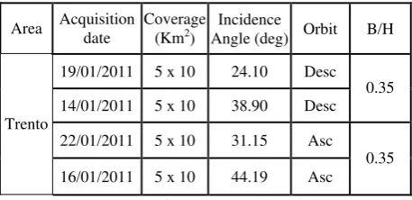
Area Acquisition date
Coverage (Km2)
Incidence
Angle (deg) Orbit B/H 19/01/2011 5 x 10 24.10 Desc
14/01/2011 5 x 10 38.90 Desc 0.35
22/01/2011 5 x 10 31.15 Asc Trento
16/01/2011 5 x 10 44.19 Asc
0.35
Table 1. Features of TerraSAR-X SpotLight imagery Two same-side stereo pairs have been considered for the DSMs generation tests, acquired on ascending and descending orbits respectively. The basic features of the images are listed in Table 1. A LiDAR airborne DSM supplied for free by the Provincia Autonoma di Trento was available as reference for the accuracy assessment.
5.2 Radargrammetric DSM analysis
Trento Absolute Error [m] on matched points - Tile 1
DSM BIAS ST.DEV. RMSE LE95 LE95 # Points
Non post-processed
Ascending 0.84 5.45 5.52 17.50 114250
Descending -1.59 4.67 4.94 14.04 137899
Post-processed (SRTM, 20 m threshold)
Ascending 0.65 4.67 4.72 13.40 108705
Descending -1.18 4.20 4.36 12.55 123037
Post-processed (SRTM, 15 m threshold)
Ascending 0.62 4.48 4.53 12.83 104756
Descending -0.83 4.20 4.28 11.24 106193
Trento Absolute Error [m] on matched points - Tile 2
DSM BIAS ST.DEV. RMSE LE95 LE95 # Points
Non post-processed
Ascending 1.28 6.96 7.08 20.42 71772
Descending -0.90 8.99 9.03 30.58 86062
Post-processed (SRTM, 20 m threshold)
Ascending 1.30 6.24 6.38 16.10 67776
Descending -0.45 6.26 6.27 17.98 71736
Post-processed (SRTM, 15 m threshold)
Ascending 1.14 5.95 6.06 15.23 63605
Descending 0.13 5.80 5.80 16.22 61851
Table 2. Trento matched points analysis results Trento DSM Absolute Error [m] - Tile 1
DSM BIAS ST.DEV. RMSE LE95 LE95 # Points
Non post-processed
Ascending -0.09 11.43 11.43 51.58 298937
Descending -1.84 5.62 5.91 17.63 289522
Merged -1.19 7.82 7.92 33.37 303522
Post-processed (SRTM, 20 m threshold)
Ascending 0.88 5.20 5.28 14.38 286049
Descending -1.23 4.56 4.72 14.61 289525
Merged -0.44 4.80 4.82 14.09 290566
Post-processed (SRTM, 15 m threshold)
Ascending 1.07 4.89 5.01 13.86 286046
Descending -0.43 4.60 4.62 13.18 289496
Merged 0.19 4.81 4.81 14.10 290533
Trento DSM Absolute Error [m] - Tile 2
DSM BIAS ST.DEV. RMSE LE95 LE95 # Points
Non post-processed
Ascending 2.54 11.30 11.59 86.69 115247
Descending -0.14 13.37 13.37 87.61 116980
Merged -1.04 9.45 9.51 29.07 117330
Post-processed (SRTM, 20 m threshold)
Ascending 1.14 7.13 7.23 20.62 115038
Descending 1.48 7.12 7.27 20.32 113771
Merged 0.27 7.42 7.42 20.50 117323
Post-processed (SRTM, 15 m threshold)
Ascending 1.48 7.12 7.27 20.32 113771
Descending 0.50 7.47 7.49 20.40 116561
Merged 1.10 7.60 7.68 21.28 116878
Table 3. Trento interpolated DSMs analysis results
At first, as mentioned before in paragraph 3, an image preprocessing step to reduce speckle noise was carried out, after the orientation performed by the rigorous model and before starting the matching procedure; to this aim, imagery has been enhanced with a 7 x 7 window Lee filter.
The accuracy assessment has been performed using DEMANAL software, developed by Prof. K. Jacobsen— Leibniz University Hannover, allowing for a full 3D comparison to remove possible horizontal biases too. The height differences are computed interpolating, with a bilinear method, the analyzed DSM over the reference LiDAR DSM; the value is negative when the extracted DSM is above the reference LiDAR DSM. The accuracy in terms of RMSE was computed at the 95% probability level (RMSE LE95), after having evaluated the LE95; therefore, the largest outliers were filtered out.
Two tiles (herein called Tile 1 and Tile 2) have been selected for the analysis, considering different morphological situations. In particular, the first one is mainly an urban area, the second includes both an urban area and forested and cultivated areas displaying a hilly topography.
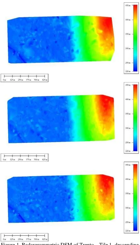
The results of the accuracy assessment are presented in Table 2. At first, the point clouds derived from the ascending and descending stereo pairs, directly produced by matching procedure without any further post-processing, have been analyzed. The accuracy is around 5.0 – 5.5 m for Tile 1, around 7.0 – 9.0 for Tile 2. Analyzing the results, some outliers have been detected in the point clouds, probably due to mismatching causing incorrect morphological reconstruction in small areas. To remove these outliers, a free available low resolution DSM (Shuttle Radar Topography Mission – SRTM DEM, 3' grid posting) has been used as reference. In details, the point clouds have been compared with SRTM, and the height differences have been computed; when the difference was greater than a fixed threshold, the corresponding point has been rejected. Two tests have been performed, using two thresholds respectively fixed at 20 m and 15 m. As shown in Table 2, an accuracy level of 4.5 m and 6 m respectively for Tile 1 and Tile 2 were obtained; the results achieved using 20 m and 15 m thresholds were not found significantly different, so that the 20 m threshold can already be considered effective for filtering out the highest errors, with a loss of matched points of about 10%. Subsequently, starting from the point clouds, three DSMs have been generated and assessed on a 2 m grid posting by a rough linear interpolation (Delaunay triangulation). In Table 3 the results of the interpolated DSMs are shown; in particular the ascending DSM is generated using the points cloud of the ascending stereo pair, the descending DSM using the points cloud of the descending one, and finally a merged DSM has been generated using a combination of the point clouds that have been previously filtered in order to remove the matched points with lower correlation (Figures 1 and 2).
In Tile 1 the accuracy is around 11 m and 6 m for the ascending and the descending DSMs respectively, and around 8 m for the merged product; after the SRTM filtering, the accuracy increases to approximately 5 m.
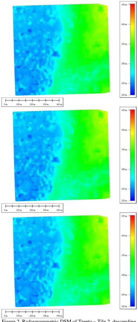
In Tile 2 the accuracy is around 11 m and 13 m for the ascending and the descending DSMs respectively, and around 9.5 m for the merged product; after the SRTM filtering, the accuracy increases to approximately 7.5 m.
The merging does not improve the results significantly, with the exception of the not processed product of Tile 2. Overall Tile 2 presented worse results than Tile 1, probably due to more complex morphologies of the area.
Figure 1. Radargrammetric DSM of Trento – Tile 1, descending (above), ascending (centre), merged (below)
6. CONCLUSIONS AND FUTURE PROSPECTS
A new model for radargrammetric processing (orientation and DSM generation) of high resolution satellite SAR stereo pairs was defined and implemented in the scientific software SISAR. An experiment was carried out over the test site of Trento (Northern Italy), where two same-side SpotLight stereo pairs have been acquired on ascending and descending orbits respectively by TerraSAR-X.
Two tiles have been selected for the accuracy analysis considering different morphological situations.
At first, the ascending and descending stereo pairs have been processed separately and the correspondingly generated point clouds have been assessed with respect to a LiDAR DSM used as reference; the accuracy was estimated around 5.0 – 5.5 m for Tile 1 and around 7.0 – 9.0 m for Tile 2.
Further, the generated point clouds have been filtered, using SRTM DEM (3' grid posting) in order to mostly remove large errors; the contribution was found effective and the accuracy increased to 4.5 m and 6 m for Tile 1 and Tile 2 respectively. Finally, complete DSMs with 2 m grid posting were generated both for Tile 1 and Tile 2, applying a rough linear interpolation (Delaunay triangulation), obtaining an accuracy of 5 m and 7.5 m respectively.
Figure 2. Radargrammetric DSM of Trento – Tile 2, descending (above), ascending (centre), merged (below)
These results are representative of the potentialities of the radargrammetric model, anyway the achievable accuracy is strictly related to the terrain morphology.
As regards future prospects of research, a more refined denoising is necessary to improve the matching reliability; therefore a deeper investigation on the expected potentiality of existing speckle filters for the high resolution SAR imagery will be carry out. Finally, alternative and more refined interpolation methods, as ordinary or multi-resolution splines (Brovelli et al., 2012), will be implemented and tested for generating a
complete DSM over a grid, also with the aim to mitigate the high frequency DSM errors which, of course, affect directly a linear interpolation as Delaunay triangulation.
References
Birchfield, S., Tomasi, C., 1999. Depth discontinuities by pixel-to-pixel stereo, Int. Journal of Computer Vision, 35 (3), pp. 269-293.
Brovelli, M., Zamboni, G., 2012. Approximation of Terrain Heights by Means of Multi-resolution Bilinear Splines, in VII Hotine-Marussi Symposium on Mathematical Geodesy, Sneeuw, N., Novák, P.;,Crespi, M., Sansò, F. (Eds.), International Association of Geodesy Symposia Volume 137, DOI: 10.1007/978-3-642-22078-4, Heidelberg, Germany: Springer-Verlag.
Capaldo, P., Crespi, M., Fratarcangeli, F., Nascetti, A., Pieralice, F., 2011. High Resolution SAR Radargrammetry. A first application with COSMO-SkyMed SpotLight Imagery, IEEE Geoscience and Remote Sensing Letters, 8 (6), pp. 1100 – 1104.
Crespi, M., Fratarcangeli, F., Giannone, F., Pieralice, F., 2009. Chapter 4—Overview on models for high resolution satellites imagery orientation, in Geospatial Technology for Earth Observation Data, D. Li, J. Shan, and J. Gong, Eds. Heidelberg, Germany: Springer-Verlag.
Hanley, H. B., Fraser, C. S., 2004. Sensor orientation for high-resolution satellite imagery: Further insights into bias-compensated RPC, in Proc. XX ISPRS Congr., Istanbul, Turkey, pp. 24–29.
Hirschmüller, H., 2008. Stereo Processing by Semi-Global Matching and Mutual Information, IEEE Transactions on Pattern Analysis and Machine Intelligence, 30(2), pp. 328-341. Méric, S., Fayard, F., Pottier, E., 2009. Chapter 20— Radargrammetric SAR image processing, in Geoscience and Remote Sensing, P.-G. P. Ho, Ed. Rijeka, Croatia: Intech. Perko, R., Raggam, H., Deutscher, J., Gutjahr, K., Schardt, M., 2011. Forest Assessment Using High Resolution SAR Data in X-Band, Remote Sensing, 3(4).
Shi, Z., Fung, K.B.,1994. A comparison of digital speckle filters. Geoscience and Remote Sensing Symposium, Surface and Atmospheric Remote Sensing: Technologies, Data Analysis and Interpretation, 4, pp. 2129-2133.
Toutin, T., 2010. Impact of RADARSAT-2 SAR Ultrafine-Mode Parameters on Stereo-Radargrammetric DEMs. IEEE Transactions on Geoscience and Remote Sensing, 48(10), pp. 3816-3823.
Zhang, L., Gruen, A., 2006. Multi-image matching for DSM generation from IKONOS imagery. ISPRS J. Photogramm. Remote Sens., 60(3), pp. 195–211.
Acknowledgements
The authors are indebted to Prof. Uwe Soergel and DLR for supplying the TerraSAR-X SpotLight imagery used in this work in the frame of the project “Evaluation of DEM derived from TerraSAR-X data” organized by the ISPRS Working Group VII/2 “SAR Interferometry”.