MEASUREMENT PRECISION AND ACCURACY OF THE CENTRE LOCATION
OF AN ELLIPSE BY WEIGHTED CENTROID METHOD
R. Matsuoka a, b a
Research and Development Division, Kokusai Kogyo Co., Ltd., 2-24-1 Harumi-cho, Fuchu, Tokyo 183-0057, JAPAN [email protected]
b
Tokai University Research & Information Center, 2-28-4 Tomigaya, Shibuya-ku, Tokyo 151-0063, JAPAN [email protected]
Commission III, WG III/1
KEY WORDS: Analysis, Measurement, Accuracy, Precision, Digital, Image, Targets
ABSTRACT:
Circular targets are often utilized in photogrammetry, and a circle on a plane is projected as an ellipse onto an oblique image. This paper reports an analysis conducted in order to investigate the measurement precision and accuracy of the centre location of an ellipse on a digital image by an intensity-weighted centroid method. An ellipse with a semi-major axis a, a semi-minor axis b, and a rotation angle of the major axis is investigated. In the study an equivalent radius r = (a2cos2+ b2sin2)1/2 is adopted as a measure of the dimension of an ellipse. First an analytical expression representing a measurement error (x, y) is obtained. Then variances Vx
of x are obtained at 1/256 pixel intervals from 0.5 to 100 pixels in r by numerical integration, because a formula representing Vx is
unable to be obtained analytically when r > 0.5. The results of the numerical integration indicate that Vx would oscillate in a 0.5
pixel cycle in r and Vx excluding the oscillation component would be inversely proportional to the cube of r. Finally an effective
approximate formula of Vx from 0.5 to 100 pixels in r is obtained by least squares adjustment. The obtained formula is a fractional
expression of which numerator is a fifth-degree polynomial of {r−0.5×int(2r)} expressing the oscillation component and denominator is the cube of r. Here int(x) is the function to return the integer part of the value x. Coefficients of the fifth-degree polynomial of the numerator can be expressed by a quadratic polynomial of {0.5×int(2r)+0.25}.
1. INTRODUCTION
Circular targets on a plane are often utilized in photogrammetry, particularly in close range photogrammetry. A circle on a plane is projected as an ellipse onto an oblique image. The centre location of an ellipse on a digital image can be estimated by centroid methods, by structural measuring methods, or by image matching methods (Luhmann et al., 2006).
This paper reports an analysis conducted in order to investigate the measurement accuracy and precision of the centre location of an ellipse on a digital image by an intensity-weighted centroid method. In the paper, an intensity-weighted centroid method is called WCM for short, an unweighted centroid method using a binary image created by thresholding is called BCM, non-iterative ellipse fitting is called NEF, iterative ellipse fitting with the star operator is called EFS, and least-squares matching is called LSM. A measurement error of the centre location of a circle or an ellipse is denoted by , and a variance of is denoted by V() in the paper.
Besides measurement errors of the centre location of an ellipse on a digital image, there is a disparity on an oblique image between the centre of the projected ellipse and the projected location of the centre of a circle. The disparity is often called an eccentricity of projection (Luhmann et al., 2006). The eccentricity exists not only in a digital image but also in an analogue image. The author showed a general formula calculating the eccentricity using the size and the location of a circle, the focal length, the position and the attitude of a camera (Matsuoka et al., 2009). The formula indicates that the eccentricity becomes larger as the circle becomes larger.
1.1 Measurement of the Centre Location of a Circle
As for a circle, the author reported an experiment in order to evaluate three measurement methods WCM, BCM, and LSM by using synthesized images of various sizes of circles (Matsuoka et al., 2009). The experiment was made by Monte Carlo simulation using 1024 synthesized images of which the centres were randomly distributed in one pixel for each circle. The radius of a circle was examined at 0.1 pixel intervals from 2 to 40 pixels. V() by WCM and BCM appeared to oscillate in an approximately 0.5 pixel cycle in radius, even though the formula to estimate the centre location of a circle by each centroid method does not seem to produce such cyclic measurement errors.
In photogrammetry some papers on the precision and/or accuracy of measurement methods of the centre location of a circle have been presented (Trinder, 1989, Trinder et al., 1995, Shortis et al., 1995). However, these papers reported experiments using limited sizes of a circle and did not indicate that the measurement precision by centroid methods may oscillate in an approximately 0.5 pixel cycle in radius.
On the other hand, in computer vision an investigation of the effect of the size of a circle on the measurement errors of its centre location by BCM was reported (Bose and Amir, 1990). A simulation on the measurement errors was executed in the study. In the simulation, 400 binarized circles were placed at 0.05 pixel intervals covering a range of one pixel in x and y direction, and the radius of a circle was examined at merely 0.25 pixel intervals. Consequently, there was no mention of finding cyclic measurement errors in the paper.
The author reported an analysis of the effect of sampling in creating a digital image on V() by WCM and BCM (Matsuoka et al., 2010). The study was conducted on the assumption that images were sampled but not quantized in digitization. Although general expressions representing V() by both methods are unable to be obtained analytically, V() were obtained by numerical integration. The results of the analysis indicated that sampling in creating a digital image would cause V() by both methods to oscillate in an approximate 0.5 pixel cycle in radius.
1.2 Measurement of the Centre Location of an Ellipse
As for an ellipse, the author conducted an experiment in order to investigate whether V() by WCM, NEF, EFS and LSM oscillates as its dimension increases (Matsuoka, 2014). The experiment was executed by Monte Carlo simulation using 1024 synthesized images of which the centres were randomly distributed in one pixel for each ellipse. Three flattenings 0.00, 0.25, 0.50, and three rotation angles 0.0°, 22.5°, 45.0° were investigated. The results clearly showed that V() by all the methods would oscillate as the dimension of an ellipse increases. Moreover the results indicated that the flattening and the rotation angle of an ellipse would affect the cycle of the oscillation of V().
Therefore the author intended to conduct an analysis in order to investigate the influence of the flatting and the rotation angle of an ellipse on the cycle of the oscillation of V() by WCM. Since the aim of the study is to investigate the basic characteristics of the oscillation of V(), the analysis was conducted on the assumption that an image is free from noise and sampled but not quantized in digitization.
In practical measurements, V() are affected by some other factors. One of the most influential factors would be quantization in creating a digital image. As for a circle, the author reported an investigation on the effect of quantization on V() by WCM (Matsuoka et al., 2011). The results of the investigation showed that V() would oscillate in an approximate 0.5 pixel cycle in radius for any quantization level and decrease as a quantization level increases. Another most influential factor would be image noises. As for a circle, the author reported an experiment on the influence of image noises on V() by using synthesized images (Matsuoka et al., 2009). The results of the experiment indicated that V() by WCM would be highly correlated to the variance of random Gaussian image noises.
2. ELLIPSE AND MEASUREMENT METHOD
2.1 Investigate Ellipse
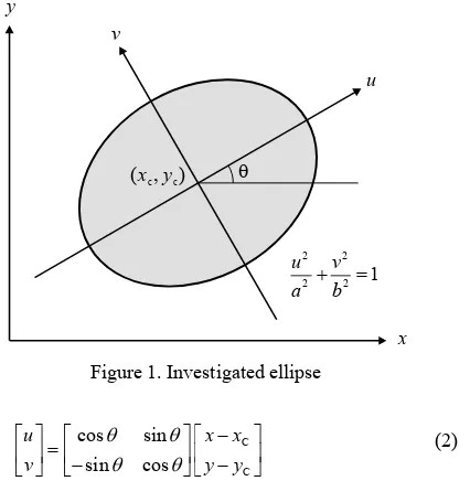
An ellipse with a semi-major axis a and a semi-minor axis b may be represented in the uv coordinate system by the following equation:
Consider that the rotation angle of the major axis is and the centre of the ellipse is located at (xC, yC) in the xy coordinate system as Figure 1 shows. The transformation from the uv system to the xy system can be written in the following equation:
Figure 1. Investigated ellipse
C
Then the investigated ellipse can be represented in the xy system by the following equation:
Rearranging Equation (3) gives the following equation:
2
2 2 2 can be written in the following equation:
From Equation (7) the following condition can be derived:
2.2 Investigated Measurement Method
The measurement method investigated in the study is an intensity-weighted centroid method which estimates the centre location (xC, yC) of a figure by using the following equation:
assumed that an image is free from noise and sampled but not quantized in digitization and a figure in the image has uniform intensity. Therefore w(i, j) is the area of part of the figure inside the region {(x, y) | ix (i+1), jy (j+1)}.3. RESULTS OF ANALYSIS
3.1 Formula of Measurement Error
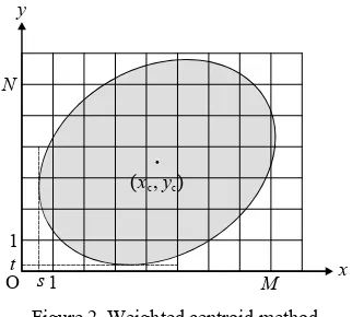
Consider that the investigated ellipse is located so that the most left and the bottom of the ellipse are x = s (0 s < 1) and y = t
Figure 2. Weighted centroid method
The estimated centre
C, C
x y of the investigated ellipse by the investigated method can be expressed as follows:
int(x) is the function to return the integer part of the value x.
Because the area of the ellipse is ab, the following equation can be obtained:
Substituting Equations (12) and (13) for Equation (10) gives the following equation:
represented by the following equation:
Then the following equations can be derived:
Substituting Equations (17) and (18) for Equation (15) gives the following equation:
obtained by substituting Equation (16) for Equation (19):
3.2 Formula of Variance of Measurement Errors
Measurement precision is usually evaluated by the variance of measurement errors. Since Equation (20) indicates that x is
independent of t and y is independent of s, the variance (Vx, Vy) decided to adopt r expressed by Equation (6) as a measure of the dimension of an ellipse and call it an equivalent radius.
I have been trying to obtain an analytical expression representing Vx. At the moment Vx is unable to be obtained
analytically if r > 1/2, while if 0 < r 1/2 the following formula was derived after many tiresome manipulations of analytical integration:
3.3 Calculation of Variance of Measurement Errors
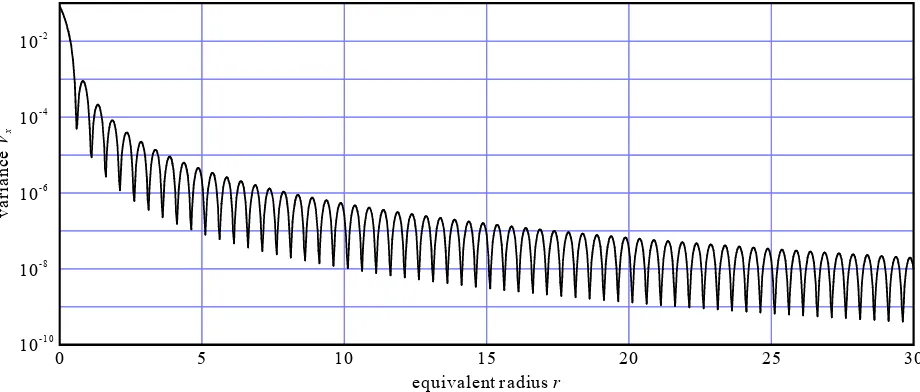
Values of Vx were calculated by Romberg integration using
Equations (20) and (21) when r > 1/2. r was examined at 1/256 (=0.00390625) pixel intervals from 0 to 100 pixels.
Figure 3 shows the calculated Vx against r. The vertical axis of
Figure 3 is expressed on a logarithmic scale. Figure 3 indicates that Vx shows a tendency to decrease gradually as r increases.
Figure 3 demonstrates that Vx would oscillate in a 0.5 pixel
cycle in r as well.
3.4 Variance excluding Oscillation Component
Here let be as follows:
where int(x) and fra(x) are the functions to return the integer and fractional parts of the value x respectively.
0 5 10 15 20 25 30
equivalent r adius r
va
Considering the oscillation of Vx I assumed that Vx would be
expressed by the following equation:
x
V A r (24)
where A() and () are functions of .
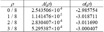
A() and () for = 0/8, 1/8, 2/8, 3/8 were obtained by least squares adjustment using Vx from 0.5 to 100 pixels in r. Table 1
shows the obtained A() and (), and Figure 4 shows the observed and approximated Vx of = 0/8, 1/8, 3/8 against r.
The vertical axis of Figure 4 is expressed on a logarithmic scale.
A() ()
0 / 8 2.543506×10⁻⁴ -2.985754 1 / 8 1.141476×10⁻⁵ -3.018711 2 / 8 2.830407×10⁻⁴ -3.011690 3 / 8 5.295387×10⁻⁴ -3.000407 Table 1. Estimated coefficients in Equation (24)
Figure 4 and Table 1 indicate that Vx excluding the oscillation
component would be inversely proportional to the cube of r.
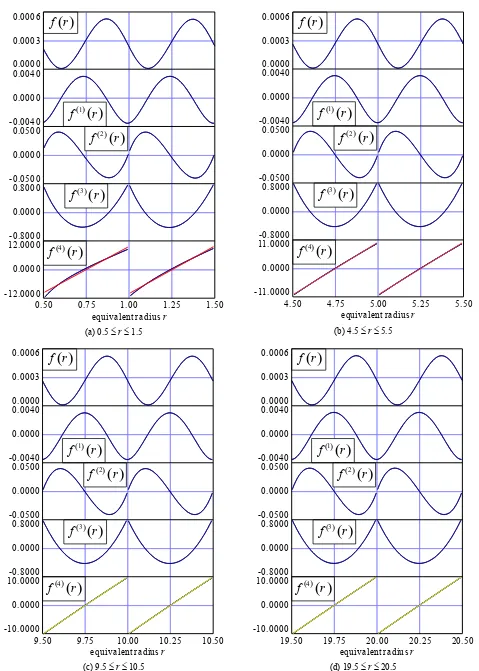
3.5 Approximate Function for Oscillation
In order to investigate the oscillation of Vx I calculated values
and divided differences of the function f(r) represented by the following equation:
3 xf r r V (25)
r was examined at 1/256 pixel intervals from 0.5 to 100 pixels. The divided differences were calculated in each 0.5 pixel interval in r.
Figure 5 shows the function values f(r), the first divided differences f (1) (r), the second ones f (2) (r), the third ones f (3) (r), and the fourth ones f (4) (r) against r. Red and yellow lines in f (4) (r) of Figure 5 show approximate linear functions of f (4) (r).
Figure 5 indicates that f (4) (r) would be approximated by a linear function with sufficient accuracy when r≥ 4.5. Although f (4) (r) seems unable to be approximated by a linear function with sufficient accuracy when 0.5 < r < 1.5, I judged that f(r) in each 0.5 pixel interval from 0.5 to 100 pixels in r would be able to be approximated by a fifth-degree polynomial of .
Let m be an integer. When m/2 r (m+1)/2, f(r) is assumed to be expressed by the following equation:
3 2 3 4 5
0m 1m 2 3 4 5
x m m m m
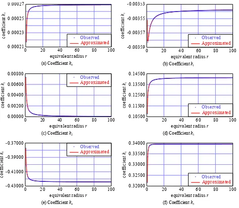
rV k k k k k k (26) The coefficients k0m, k1m, ..., k5m (1 m 199; 0.5 r 100)
were obtained by least squares adjustment. Figure 6 shows obtained k0m, k1m, ..., k5m against r.
Here let n be an integer and 0 n 5. kn is assumed to be
expressed by the following equation:
2 0 1 2
1 1
n n n n
k l l l
r r
(27)
where r is the equivalent radius of the midpoint in 0.5 pixel interval, which is expressed as follows:
int 2 1 1
2 4 4
r
r r (28)
The coefficients l00, l01,..., l52 were obtained by least squares adjustment. Table 2 shows the obtained l00, l01,..., l52. Red lines in Figure 6 show approximate values of k0m, k1m,..., k5m
calculated by using the obtained l00, l01,..., l52.
n ln0 ln1 ln2
0 2.696364×10⁻⁴ -3.003633×10⁻⁵ -7.029158×10⁻⁶ 1 -3.536622×10⁻³ -1.222481×10⁻⁴ 8.277960×10⁻⁵ 2 1.968267×10⁻⁷ 5.021470×10⁻³ 3.683751×10⁻⁴ 3 1.414640×10⁻¹ -1.891441×10⁻² -4.744025×10⁻³ 4 -4.243913×10⁻¹ 1.834941×10⁻² 1.285956×10⁻² 5 3.395103×10⁻¹ 7.704924×10⁻⁴ -1.055554×10⁻²
Table 2. Estimated coefficients in Equation (27)
0 20 40 60 80 100
equivalent r adius r
va
ri
a
nc
e
Vx 10- 3
10- 5
10- 7
10- 9
10- 11
observed
approximated
Vx = 2 .5435 x 1 0-04 -2 .98 58
r
Vx = 1 .1415 x 1 0
-05 -3 .01 87
r
Vx = 5 .2954 x 1 0-04 -3 .000 4
r
Figure 4. Variance Vx of = 0/8, 1/8, 3/8 vs. equivalent radius r (0.5 r 100)
0.50 0.75 1.00 1.25 1.50
equivalent r adius r -12.0000
4.50 4.75 5.00 5.25 5.50
equivalent radius r (b) 4.5 r 5.5
9.50 9.75 10.00 10.25 10.50
equivalent r adius r -10.0000
19.50 19.75 20.00 20.25 20.50
equivalent r adius r -10.0000
0.0000 10.0000
(d) 19.5 r 20.5 Figure 5. Function f(r) and its divided differences f (1) (r), f (2) (r), f (3) (r), f (4) (r) vs. equivalent radius r
Figure 6 indicates that all coefficients except k1 would be approximated with sufficient accuracy by Equation (27). As for k1, although there is a small discrepancy at r 0.75, all except
0.75
r would be approximated with sufficient accuracy by Equation (27). Consequently I judged that k0, k1, ..., k5 would be able to be approximated by Equation (27).
3.6 Approximate Formula of Measurement Precision
Finally an approximate formula of Vx when r > 0.5 was
obtained. The obtained formula is as follows:
2 3 4 5
int(x) is the function to return the integer part of the value x.
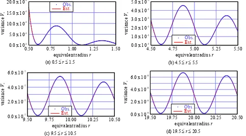
By using the obtained formula (29) I calculated Vx at 1/256
pixel intervals from 0.5 to 100 pixels in r. Some of the calculated results are shown in Figure 7. Blue dots “Obs.” in Figure 7 show Vx by the numerical integration, while red lines
“Est.” in Figure 7 show Vx by the approximation.
The maximum absolute approximation error was 4.640×10⁻⁶ (1.732094×10⁻³ by the numerical integration, 1.736734×10⁻³ by the approximation) at r = 0.5. A root mean squares of errors (RMSE) Vx1/2 by the numerical integration and by the
approximation at r = 0.5 is 0.041618 pixels and 0.041674 pixels respectively. The difference between two values is merely 0.000056 pixels.
From the results I concluded that the obtained approximation formula of Vx would be effective enough.
0.00021 0.00023 0.00025 0.00027
0 20 40 60 80 100
equivalent radius r
Approximated
(a) Coefficient k0
-0.00359 -0.00357 -0.00355 -0.00353
0 20 40 60 80 100
equivalent r adius r
Approximated
equivalent radius r
Approximated
equivalent radius r
Approximated
equivalent r adius r
Approximated
(e) Coefficient k4
0.32000
equivalent radius r
Approximated
(f) Coefficient k5 Figure 6. Coefficients kn vs. equivalent radius r (0.5 r 100)
4. CONCLUSIONS
I succeeded in obtaining the formula representing the measurement error (x, y) of the centre location of an ellipse
with a semi-major axis a, a semi-minor axis b, and a rotation angle of the major axis by the intensity-weighted centroid method.
An equivalent radius r = (a2cos2+ b2sin2)1/2 was adopted as a measure of the dimension of an ellipse in the analysis of the variance Vx of x. Although I succeeded in obtaining the
analytical expression representing Vx when r 0.5, I failed in
obtaining an analytical expression representing Vx when r > 0.5.
I conducted numerical integration to obtain Vx at 1/256 pixel
intervals from 0.5 to 100 pixels in r. The results of the numerical integration indicate that Vx would oscillate in a 0.5
pixel cycle in r and Vx excluding the oscillation component
would be inversely proportional to the cube of r.
I succeeded in obtaining an effective approximate formula of Vx
from 0.5 to 100 pixels in r as well. The obtained formula is a fractional expression of which numerator is a fifth-degree polynomial of {r−0.5×int(2r)} expressing the oscillation component and denominator is the cube of r. Coefficients of the fifth-degree polynomial of the numerator can be expressed by a quadratic polynomial of {0.5×int(2r)+0.25}.
REFERENCES
Bose, C. B. and Amir, I., 1990. Design of Fiducials for Accurate Registration Using Machine Vision, IEEE Transactions on Pattern Analysis and Machine Intelligence, 12(12), pp. 1196-1200.
Luhmann, T., Robson, S., Kyle, S. and Harley, I., 2006. Close Range Photogrammetry, Whittles Publishing, Caithness, UK, pp. 186-188, pp. 364-376.
Matsuoka, R., Sone, M., Sudo, N., Yokotsuka, H. and Shirai, N., 2009. Comparison of Measuring Methods of Circular Target Location, Journal of the Japan Society of Photogrammetry and Remote Sensing, 48(3), pp. 154-170.
Matsuoka, R., Sone, M., Sudo, N., Yokotsuka, H. and Shirai, N., 2010. Effect of Sampling in Creating a Digital Image on Measurement Accuracy of Center Location of a Circle, The International Archives of the Photogrammetry, Remote Sensing and Spatial Information Sciences, Paris, France, Vol. XXXVIII, Part 3A, pp. 31-36.
Matsuoka, R., Shirai, N., Asonuma, K., Sone, M., Sudo, N. and Yokotsuka, H., 2011. Measurement Accuracy of Center Location of a Circle by Centroid Method, Photogrammetric Image Analysis, LNCS Volume 6952, Springer-Verlag, Heidelberg, Germany, pp. 297-308.
Matsuoka, R., 2014. Oscillation of the Measurement Accuracy of the Center Location of an Ellipse on a Digital Image, The International Archives of the Photogrammetry, Remote Sensing and Spatial Information Sciences, Zurich, Switzerland, Vol. XL-3, pp. 211-218.
Shortis, M. R., Clarke, T. A. and Robson, S., 1995. Practical Testing of the Precision and Accuracy of Target Image Centring Algorithms. Videometrics IV, SPIE Vol. 2598, pp. 65-76.
Trinder, J. C., 1989. Precision of Digital Target Location, Photogrammetric Engineering and Remote Sensing, 55(6), pp. 883-886.
Trinder, J. C., Jansa, J. and Huang, Y., 1995. An Assessment of the Precision and Accuracy of Methods of Digital Target Location, ISPRS Journal of Photogrammetry and Remote Sensing, 50(2), pp. 12-20.
0.50 0.75 1.00 1.25 1.50
equivalent radius r
Est.
4.50 4.75 5.00 5.25 5.50
equivalent r adius r (b) 4.5 r 5.5
9.50 9.75 10.00 10.25 10.50
equivalent r adius r
Est. Obs.
(c) 9.5 r 10.5
19.50 19.75 20.00 20.25 20.50
equivalent r adius r 6.0 x 1 0- 8
Figure 7. Variance Vx vs. equivalent radius r