24 (2000) 165}188
Complementarity problems in GAMS
and the PATH solver
Michael C. Ferris*, Todd S. Munson
Computer Sciences Department, University of Wisconsin}Madison, 1210 West Dayton Street,
Madison, WI 53706, USA
Received 1 September 1998; accepted 1 December 1998
Abstract
A fundamental mathematical problem is to "nd a solution to a square system of
nonlinear equations. There are many methods to approach this problem, the most
famous of which is Newton's method. In this paper, we describe a generalization of this
problem, the complementarity problem. We show how such problems are modeled within the GAMS modeling language and provide details about the PATH solver,
a generalization of Newton's method, for"nding a solution. While the modeling format is
applicable in many disciplines, we draw the examples in this paper from an economic background. Finally, some extensions of the modeling format and the solver are
de-scribed. 2000 Elsevier Science B.V. All rights reserved.
JEL classixcation: C63
Keywords: Complementarity problems; Variational inequalities; Algorithms
1. Introduction
Modeling languages are becoming increasingly important to application developers as the problems considered become more complex. Modeling languages such as AMPL or GAMS o!er an environment tailored to expressing
*Corresponding author.; e-mail: [email protected].
This material is based on research supported by National Science Foundation Grant CCR-9619765 and GAMS Corporation. The paper is an extended version of a talk presented at CEFES
'98 (Computation in Economics, Finance and Engineering: Economic Systems) in Cambridge,
England, in July 1998.
mathematical constructs. They can e$ciently manage a large volume of data
and allow users to concentrate on the model rather than the solution methodo-logy. Over time, modeling languages have evolved and adapted as new algo-rithms and problem classes have been explored.
A fundamental mathematical problem is to"nd a solution to a square system
of nonlinear equations. Newton's method, perhaps the most famous solution
technique, has been extensively used in practice to calculate a solution. Two generalizations of nonlinear equations are very popular with modelers, the constrained nonlinear system (that incorporates bounds on the variables), and the complementarity problem.
The complementarity problem adds a combinatorial twist to the classic square system of nonlinear equations, thus enabling a broader range of situ-ations to be modeled. For example, the complementarity problem can be used to model the Karush}Kuhn}Tucker (KKT) optimality conditions for nonlinear
programs (Karush, 1939; Kuhn and Tucker, 1951), Wardropian and Walrasian equilibria (Ferris and Pang, 1997b), and bimatrix games (Lemke and Howson, 1964). One popular solver for these problems, PATH, is based upon a generaliz-ation of the classical Newton method. This method has achieved considerable success on practical problems.
In this paper, we study the complementarity problem from a modeling perspective with emphasis on economic examples, show how to model such problems within the GAMS modeling language, and provide details about the PATH solver. We will assume an elementary understanding of linear program-ming, including basic duality theory, and a working knowledge of the GAMS modeling system (Brooke et al., 1988).
We begin developing the complementarity framework by looking at the KKT conditions for linear programs. We discuss the adaptations made in GAMS to support the complementarity problem class and provide some additional exam-ples. Section 3 continues by elaborating on the PATH solver, available options, and output. Finally some extensions of the modeling format and additional uses of the solver are given.
2. Complementarity problems
The transportation model is a simple linear program where demands for a single good must be satis"ed by suppliers at minimal transportation cost. The
underlying transportation network is given as a setAof arcs and the problem variables are the amountsx
GHto be shipped over each arc (i,j)3A. The linear
program can be written mathematically as
Herec
GHis the unit shipment cost on the arc (i,j) connecting nodesiandj,sGis the
supply capacity atiandd
His the demand at j.
Associated with each constraint is a multiplier, alternatively termed a dual variable or shadow price. These multipliers represent the marginal price on changes to the corresponding constraint. If we label the prices on the supply constraintpQ and those on the demand constraintpB, then intuitively, at each supply nodei
pay for more supply fromi, thuspQG"0. We write these conditions succinctly as:
04pQGNs
G5
HGHZA
xGH, ∀i
where theNnotation is understood to mean that at least one of the adjacent inequalities must be satis"ed as an equality. For example, either 0"pQG or
s
andpBH"0 if there is excess supply, that is
GGHZAxGH'dH. Clearly the supply
price atiplus the transportation costc
GHfromitojmust exceed the market price
atj, that ispQG#c
GH5pBH. Furthermore, if the cost of delivery strictly exceeds the
market price, that is pQG#c
GH'pBH, then nothing is shipped fromi toj, so that x
GH"0. An equivalent, but more succinct notation for all the above conditions is
04pQGNs
Conditions (2) de"ne a linear complementarity problem that is easily
recog-nized as the complementary slackness conditions of the linear program (1). For linear programs the complementary slackness conditions are both necessary and su$cient forxto be an optimal solution of the problem (1). Furthermore,
conditions (2) are also the necessary and su$cient optimality conditions for
a related problem in the variables (pQ,pB)
termed the dual linear program (hence the nomenclature &dual variables').
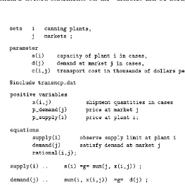
Fig. 1. A simple MCP model in GAMS,transmcp.gms.
complementarity problems. A solution of Eq. (2) tells us the arcs used to transport goods. A priori we do not need to specify which arcs to use, the solution itself indicates them. This property represents the key contribution of a complementarity problem over a system of equations. If we know what arcs to send#ow down, we can just solve a simple system of linear equations. However,
the key to the modeling power of complementarity is that it chooses which of the inequalities in Eq. (2) to satisfy as equations. In economics we can use this property to generate a model with di!erent regimes and let the solution
deter-mine which ones are active. A regime shift could, for example, be a back stop technology like windmills that become pro"table if a CO
tax is increased.
The GAMS code for the complementarity version of the transportation problem is given in Fig. 1; the actual data for the model is assumed to be given in the"letransmcp.dat. Note that the model written corresponds very closely to
Eq. (2). In GAMS, theNsign is replaced in themodelstatement with a&.'. It is
precisely at this point that the pairing of variables and equations shown in Eq. (2) occurs in the GAMS code, so that in the example, the function de"ned by
rationalis complementary to the variablex. To inform a solver of the bounds,
(for a declared variablez(i)):
z.lo(i)"0;
or
positive variable z;
Further information on the GAMS syntax can be found in Rutherford (1995); more examples of problems written using the complementarity problem are found in MCPLIB (Dirkse and Ferris, 1995a). Finally, note that GAMS requires the modeler to write F(z)"g"0 whenever the complementary variable is
lower bounded, and does not allow the alternative form0"l"F(z).
While many interior point methods for linear programming exploit this complementarity framework (so-called primal}dual methods), the real power of
this modeling format is the new problem instances it enables a modeler to create. We now show some examples of how to extend the simple model (2) to investigate other issues and facets of the problem at hand.
Demand in the model of Fig. 1 is independent of the pricesp. Since the prices
pare variables in the complementarity problem (2), we can easily replace the constant demanddwith a functiond(p). Clearly, any algebraic function ofpthat can be expressed in GAMS can now be added to the model given in Fig. 1. For example, a linear demand function could be expressed using
GGHZA x
GH5d
H(1!pBH) ∀j.
Note that the demand is rather strange ifpBHexceeds 1. Other more reasonable examples ford(p) are easily derived from Cobb}Douglas or CES utilities. For
those examples, the resulting complementarity problem becomes nonlinear in the variables p. Details of complementarity for more general transportation models can be found in Dirkse and Ferris (1998b) and Ferris et al. (1998b).
Another feature that can be added to this model are tari!s or taxes. In the case
where a tax is applied at the supply point, the third general inequality in Eq. (2) is replaced by
pQG(1#t
G)#c
GH5pBH ∀(i,j)3A.
The taxes can be made endogenous to the model, details are found in Rutherford (1995). The key point to make is that with either of the above modi"cations, the
complementarity problem is not just the optimality conditions of a linear program. In fact, in many cases, there is no optimization problem corresponding to the complementarity conditions.
Fig. 2. Walrasian equilibrium as an NCP,walras1.gms.
(NCP) Given a functionF:RLPRL,"ndz3RLsuch that
04zNF(z)50.
Recall that theNsign signi"es that one of the inequalities is satis"ed as an
equality, so that componentwise,z
GFG(z)"0. We frequently refer to this
prop-erty asz
Gis&complementary'toF
G. A special case of the NCP that has received
much attention is when F is a linear function, the linear complementarity problem (Cottle et al., 1992).
A Walrasian equilibrium can also be formulated as a complementarity prob-lem (see Mathiesen, 1987). In this case, we want to"nd a pricep3RKand an
activity levely3RLsuch that
04yN¸(p) :"!A2p50,
04pNS(p,y) :"b#Ay!d(p)50. (3)
Here,S(p,y) represents the excess supply function, and¸(p) represents the loss
function. Complementarity allows us to choose the activitiesy
Hto run (i.e. only
those that do not make a loss). The second set of inequalities state that the price of a commodity can only be positive if there is no excess supply. These conditions indeed correspond to the standard exposition of Walras'law which
states that supply equals demand if we assume all pricespwill be positive at a solution. Formulations of equilibria as systems of equations do not allow the model to choose the activities present, but typically make an a priori assumption on this matter. A GAMS implementation of Eq. (3) is given in Fig. 2.
Many large-scale models of this nature have been developed. An interested modeler could, for example, see how a large-scale complementarity problem was used to quantify the e!ects of the Uruguay round of talks (Harrison et al., 1997).
In many modeling situations, a key tool for clari"cation is the use of
Fig. 3. Walrasian equilibrium as an MCP,walras2.gms.
corresponding to the demand functiond(p) in the Walrasian equilibrium (3). The syntax for carrying this out is shown in Fig. 3. We use the variablesdto store the demand function referred to in the excess supply equation. The modelwalras
now contains a mixture of equations and complementarity constraints. Since constructs like the above are prevalent in many practical models, the GAMS syntax allows such formulations.
Note that positive variables are paired with inequalities, while free variables are paired with equations. A crucial point misunderstood by many experienced modelers is thatthe bounds on thevariable determine the relationships satisxed by
the function F. Thus, a mixed complementarity problem (MCP) is speci"ed by
three pieces of data, namely the lower boundsl, the upper boundsuand the functionF.
(MCP) Given lower boundsl3+R6+!R,,L, upper bounds u3+R6+R,,L
and a functionF:RLPRL, "ndz3RLsuch that precisely one of the
following holds for eachi3+1,2,n,:
F
G(z)"0 and l
G4z
G4u
G
F
G(z)'0 and z
G"l
G
F
G(z)(0 and z
G"u
G.
These relationships de"ne a general MCP (sometimes termed a rectangular
variational inequality (Harker and Pang, 1990)).
Note that the NCP is a special case of the MCP. For example, to formulate an NCP in the GAMS/MCP format we set
or declare
positive variable z;
Another special case is a square system of nonlinear equations
(NE) Given a functionF:RLPRL"ndz3RLsuch that:
F(z)"0.
In order to formulate this in the GAMS/MCP format we just declare
free variable z;
In both the above cases, wemust notmodify the lower and upper bounds on the variables later (unless we wish to drastically change the problem under consideration).
A simpli"cation is allowed to the model statement in Fig. 3. In many cases, it
is not signi"cant to match free variables explicitly to equations; we only require
that there are the same number of free variables as equations. Thus, in the example of Fig. 3, the model statement could be replaced by
model walras / demand,S.p, L.y /;
GAMS generates a list of all variables appearing in the equations found in the model statement, performs explicitly de"ned pairings and then checks that the
number of remaining equations equals the number of remaining free variables. All variables that are not free and all inequalities must be explicitly matched. This extension allows existing GAMS models consisting of a square system of nonlinear equations to be easily recast as a complementarity problem } the
model statement is unchanged.
An advantage of the extended formulation described above is the pairing between&"xed'variables (ones with equal upper and lower bounds) and a
com-ponent ofF. If a variablez
Gis"xed, thenF
G(z) is unrestricted since precisely one
of the three conditions in the MCP de"nition automatically holds when
zG"l
G"u
G. Thus if a variable is"xed in a GAMS model, the paired equation is
completely dropped from the model. This convenient modeling trick can be used to remove particular constraints from a model at generation time. As an example, in economics,"xing a level of production will remove the zero-pro"t
condition for that activity.
Modelers typically add bounds to their variables when attempting to solve nonlinear problems in order to restrict the domain of interest. For example, many square nonlinear systems are formulated as
F(z)"0, l4z4u,
note the distinction between MCP and CNS. The MCP uses the bounds to infer relationships on the function F. If a "nite bound is active at a solution, the
corresponding component ofFis only constrained to be nonnegative or non-positive in the MCP, whereas in CNS it must be zero. Thus there may be many solutions of MCP that do not satisfyF(z)"0. Only ifzHis a solution of MCP
withl(zH(uis it guaranteed that F(zH)"0.
Simple bounds on the variables are a convenient modeling tool that translates into e$cient mathematical programming tools. For example, specialized codes
exist for the bound constrained optimization problem
minf(x) subject tol4x4u.
The"rst order optimality conditions of this problem are precisely MCP(f(x),
[l,u]). We can easily see this condition in a one-dimensional setting. If we are at an unconstrained stationary point, thenf(x)"0. Otherwise, ifxis at its lower
bound, then the function must be increasing as x increases, so f(x)50.
Conversely, ifxis at its upper bound, then the function must be increasing as
xdecreases, so thatf(x)40. The MCP allows such problems to be easily and
e$ciently processed.
Upper bounds can be used to extend the utility of existing models. For example, in Fig. 3 it may be necessary to have an upper bound on the activity levely. In this case, we simply add an upper bound toyin the model statement, and replace the loss equation with the following de"nition:
y.up(j)"10;
L(j).. -sum(i,p(i)*A(i,j))"e"0;
Here, for bounded variables, we do not know beforehand if the constraint will be satis"ed as an equation, less than inequality or greater than inequality, since this
determination depends on the values of the solution variables. We adopt the convention that all bounded variables are paired to equations. Further details on this point are given in Section 3.1. However, let us interpret the relationships that the above change generates. Ify
H"0, the loss function can be positive since
we are not producing in thejth sector. Ify
His strictly between its bounds, then
the loss function must be zero by complementarity; this is the competitive assumption. However, ify
His at its upper bound, then the loss function can be
negative. Of course, if the market does not allow free entry, some "rms may
operate at a pro"t (negative loss). For more examples of problems, the interested
reader is referred to Dirkse and Ferris (1995a) and Ferris and Pang, (1997a,b).
3. The PATH solver
against which new MCP solvers are compared (Billups et al., 1997). The core algorithm is a nonsmooth Newton method (Robinson, 1994) to"nd a zero of the
normal map (Robinson, 1992)
F(n(x))#x!n(x)
associated with the MCP. Heren(x) represents the projection ofxonto [l,u] in the Euclidean norm. Ifxis a zero of the normal map, thenn(x) solves the MCP. A nonmonotone pathsearch (Dirkse and Ferris, 1996; Ferris and Lucidi, 1994) using the residual of the normal map
""F(n(x))#x!n(x)""
as a merit function can be used to improve robustness. Rather than repeat mathematical results from elsewhere, we note that proof of convergence and rate of convergence results can be found in Ralph (1994), while technical details of the implementation of the code and interfaces to other software packages are given in Ferris and Munson (1998b). The remainder of this section attempts to describe the algorithm features and enhancements from the perspective of a modeler.
To this end, we will assume for the remainder of this paper that the modeler has created a "le named transmcp.gms which de"nes an MCP model
transportusing the GAMS syntax described in Section 2. Furthermore, we
will assume the modeler is using PATH for solving the MCP at hand. There are two ways to ensure that PATH is used as opposed to any other GAMS/MCP solver. These are as follows:
(1) Add the following line to the transmcp.gms "le prior to the solve
statement
option mcp"path;
PATH will then be used instead of the default solver provided.
(2) Rerun the gamsinst program from the GAMS system directory and choose PATH as the default solver for MCP.
To solve the problem, the modeler executes the following command:
gams transmcp
Heretransmcpcan be replaced by any"lename containing a GAMS model.
Many other command line options for GAMS exist; the reader is referred to Brooke et al. (1988) for further details.
At this stage, a log ("le) is generated that provides details of what GAMS and
terminates, a listing"le is also generated. We now describe the output in the
listing"le speci"cally related to the complementarity problem and PATH.
3.1. The listingxle
The listing"le is the standard GAMS mechanism for reporting model results.
This"le contains information regarding the compilation process, the form of the
generated equations in the model, and a report from the solver regarding the solution process.
We now detail the last part of this output for the PATH solver, an example of which is given in Fig. 4. We use &2' to indicate where we have omitted
continuing similar output.
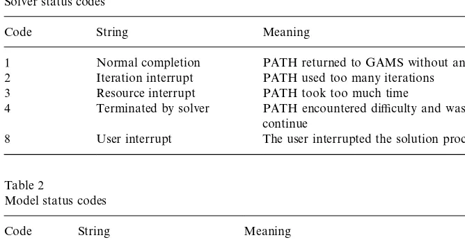
After a summary line indicating the model name and type and the solver name, the listing"le shows a solver status and a model status. Tables 1 and
2 display the relevant codes that are returned by PATH under di!erent
circum-stances. A modeler can access these codes within thetransmcp.gms"le using
transport.solstatandtransport.modelstat, respectively.
After this, a listing of the time and iterations used is given, along with a count on the number of evaluation errors encountered. If the number of evaluation errors is greater than zero, further information can typically be found later in the listing "le, prefaced by &****'. Information provided by the solver is then
displayed.
Next comes the solution listing, starting with each of the equations in the model. For each equation passed to the solver, four columns are reported, namely the lower bound, level, upper bound and marginal. GAMS moves all parts of a constraint involving variables to the left-hand side, and accumulates the constants on the right-hand side. The lower and upper bounds correspond to the constants that GAMS generates. For equations, these should be equal, whereas for inequalities one of them should be in"nite. The level value of the
equation (an evaluation of the left-hand side of the constraint at the current point) should be between these bounds, otherwise the solution is infeasible and the equation is marked as follows:
seattle .chicago!0.153!2.000#INF 300.000 INFES
The&marginal'column on an equation returns the level value of the variable that
was paired with this equation. If the modeler did not pair a particular equation with a variable, the value returned here corresponds to the variable that GAMS paired with the equation.
Unfortunately, this is not the end of the story. Some equations may have the following form:
LOWER LEVEL UPPER MARGINAL
Table 1
Solver status codes
Code String Meaning
1 Normal completion PATH returned to GAMS without an error 2 Iteration interrupt PATH used too many iterations
3 Resource interrupt PATH took too much time
4 Terminated by solver PATH encountered di$culty and was unable to
continue
8 User interrupt The user interrupted the solution process
Table 2
Model status codes
Code String Meaning
1 Optimal PATH found a solution of the problem 6 Intermediate infeasible PATH failed to solve the problem
This should be construed as a warning from GAMS, as opposed to an error. The
REDEFonly occurs if the paired variable to the constraint had a"nite lower
and upper bound and the variable is at one of those bounds, since at the solution of the complementarity problem the &equation' may not be satis"ed. The
problem occurs because of a limitation in the GAMS syntax for complementar-ity problems. The GAMS equations are used to de"ne the function F. The
bounds on the function F are derived from the bounds on the associated variable. Before solving the problem, for "nite bounded variables, we do not
know if the associated function will be positive, negative or zero at the solution. Thus, we do not know whether to de"ne the equation as &"e"', &"l"' or &"g"'. GAMS therefore allows any of these, and informs the modeler via the &REDEF' label that internally GAMS has rede"ned the bounds so that the
solver processes the correct problem, but that the solution given by the solver does not satisfy the original bounds.Note that this is not an error, just a warning. The solver has solved the complementarity problem specixed by this equation.
GAMS gives this report to ensure that the modeler understands that the complementarity problem derives the relationships on the equations from the bounds, not from the equation de"nition.
internally matched constraint slack. The de"nition of this slack is the minimum
of equ.l}equ.lower and equ.l}equ.upper, where equ is the paired equation.
Finally, a summary report is given that indicates how many errors were found. Fig. 4 is a good case; when the model has infeasibilities, these can be found by searching for the string&INFES' as described above.
3.2. The logxle
We will now describe the behavior of the PATH algorithm in terms of the output typically displayed when using the code. An example of the log for a particular run is given as Fig. 5.
The"rst few lines on this log"le are printed by GAMS during its compilation
and generation phases. The model is then passed o!to PATH at the stage where
the&Executing PATH'line is written out. After some basic memory allocation
and problem checking, the PATH solver checks if the modeler required an option"le to be read. In the example this is not the case. If it is directed to read
an option"le (see Section 3.4 below), then the following output is generated after
the PATH banner.
Reading options file PATH.OPT
'output
}linear}model yes;
Options: Read: Line 2 invalid: hi}there;
Read of options file complete.
If the option reader encounters an invalid option (as above), it reports this but carries on executing the algorithm. Following this, the algorithm starts solving the problem.
The "rst phase of the code is a crash procedure attempting to quickly
determine which of the inequalities should be active. This procedure is documented fully in Dirkse and Ferris (1997). The"rst column of the crash log is
just a label indicating the current iteration number, the second gives an indica-tion of how many funcindica-tion evaluaindica-tions have been performed so far. Note that precisely one Jacobian (gradient) evaluation is performed per crash iteration. The number of changes to the active set between iterations of the crash procedure is shown under the&di! 'column. The crash procedure terminates if
this becomes small. Each iteration of this procedure involves a factorization of a matrix whose size is shown in the next column. The residual is a measure of how far the current iterate is from satisfying the complementarity conditions (MCP); it is zero at a solution. See Section 3.6 for further information. The column&step' corresponds to the steplength taken in this iteration!ideally
this should be 1. If the factorization fails, then the matrix is perturbed by an identity matrix scaled by the value indicated in the&prox' column. The&label'
Fig. 5. Log File from PATH for solvingtransmcp.gms.
conditions (MCP). Typically, relatively few crash iterations are performed. Section 3.4 gives mechanisms to a!ect the behavior of these steps.
After the crash is completed, the main algorithm starts shown by the&Major
Iteration Log' #ag. The columns that have the same labels as in the crash log
columns that we now explain. Each major iteration attempts to solve a linear mixed complementarity problem using a pivotal method that is a generalization of Lemke's method (Lemke and Howson, 1964). The number of pivots
per-formedpermajor iteration is given in the&minor'column.
If more than 500 pivots are performed, a minor log is output that gives more details of the status of these pivots. In particular, the number of problem variablesz, slack variables corresponding to variables at lower boundwand at upper boundvare noted. Arti"cial variables are also noted in this minor log, see
Ferris and Munson (1998b) for further details. Again, the option"le can be used
to a!ect the frequency of such output.
The&grad'column gives the cumulative number of Jacobian evaluations used;
typically one evaluation is performed per iteration. The&inorm'column gives the
value of the error in satisfying the equation indicated in the&label'column.
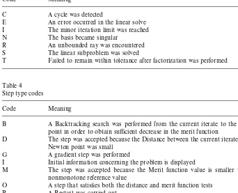
At each iteration of the algorithm, several di!erent step types can be taken. In
order to help the PATH user, we have added two code letters indicating the return code from the linear solver and the step type to the log "le. Table 3
explains the return codes for the linear solver and Table 4 explains the meaning of each step type.
At the end of the log "le, summary information regarding the algorithm's
performance is given. The string&**EXIT}solution found'. is an indication that
PATH solved the problem. Any other EXIT string indicates a termination at a point that may not be a solution. These strings give an indication of what
modelstatandsolstatwill be returned to GAMS. After this, the&Restarting
execution' #ag indicates that GAMS has been restarted and is processing the
results passed back by PATH. Currently, features to detect ill-posed, poorly scaled, or singular models are being incorporated into PATH (Ferris and Munson, 1998a).
3.3. The statusxle
If for some reason the PATH solver exits without writing a solution, or
thesysout#ag is turned on, the status"le generated by the PATH solver will be
reported in the listing"le. The status"le is similar to the log"le, but provides
more detailed information. The modeler is typically not interested in this output.
3.4. Options
The default options of PATH should be su$cient for most models; the
techniques for changing these options are now described. To change the default options on the model transport, the modeler is required to write a "le
path.optin the same directory as the model resides and either add a line
Table 3
Linear solver codes
Code Meaning
C A cycle was detected
E An error occurred in the linear solve I The minor iteration limit was reached N The basis became singular
R An unbounded ray was encountered S The linear subproblem was solved
T Failed to remain within tolerance after factorization was performed
Table 4 Step type codes
Code Meaning
B A Backtracking search was performed from the current iterate to the Newton point in order to obtain su$cient decrease in the merit function
D The step was accepted because the Distance between the current iterate and the Newton point was small
G A gradient step was performed
I Initial information concerning the problem is displayed
M The step was accepted because the Merit function value is smaller than the nonmonotone reference value
O A step that satis"es both the distance and merit function tests
R A Restart was carried out
W A Watchdog step was performed in which we returned to the last point encoun-tered with a better merit function value than the nonmonotone reference value (M, O, or B step), regenerated the Newton point, and performed a backtracking search
before thesolvestatement in the"letransmcp.gms, or use the command-line
option
gams transmcp optfile"1
We give a list of the available options along with their defaults and meaning in Tables 5 and 6. Note that only the "rst three characters of every word are
signi"cant.
GAMS controls the total number of pivots allowed via theiterlimoption. If more pivots are needed for a particular model then either of the following lines should be added to thetransmcp.gms"le before the solve statement
option iterlim"2000;
Table 5 PATH options
Option Default Explanation
convergence}tolerance 1e-6 Stopping criterion
crash}iteration}limit 50 Maximum iterations allowed in crash crash}method Pnewton pnewton or none
crash}minimum}dimension 1 Minimum problem dimension to perform crash
crash}nbchange}limit 1 Number of changes to the basis allowed crash}searchtype Arc Searchtype to use in the crash method. cumulative}iteration}limit 10000 Maximum minor iterations allowed gradient}searchtype Arc Searchtype to use when a gradient step is
taken
gradient}step}limit 5 Maximum number of gradient step allowed
before restarting
lemke}start Automatic Frequency of lemke starts (automatic, "rst,
always)
major}iteration}limit 500 Maximum major iterations allowed merit}function Fischer Merit function to use (normal or"scher)
minor}iteration}limit 1000 Maximum minor iterations allowed in each major iteration
nms Yes Allow line/path searching, watchdoging, and nonmonotone descent
nms}initial}reference}factor 20 Controls size of initial reference value nms}memory}size 10 Number of reference values kept
nms}mstep}frequency 10 Frequency at whichmsteps are performed
Similarly if the solver runs out of memory, then the workspace allocated can be changed using
transport.workspace"20;
The above example would allocate 20MB of workspace for solving the model. Problems with a singular basis matrix can be overcome by using the
proximal}perturbation option (Billups and Ferris, 1997), and linearly
de-pendent columns can be output with the output}factorization}
singu-laritiesoption.
In particular, PATH can emulate Lemke's method (Cottle and Dantzig, 1968;
Lemke and Howson, 1964) for LCP with the following options:
crash}method none;
major}iteration}limit 1;
lemke}start first;
nms no;
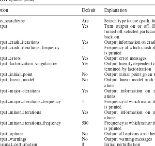
Table 6
PATH options (cont)
Option Default Explanation
nms}searchtype Arc Search type to use (path, line, or arc)
output Yes Turn output on or o!. If output is
turned o!, selected parts can be turned
back on.
output}crash}iterations Yes Output information on crash iterations output}crash}iterations}frequency 1 Frequency at which crash iteration log
is printed
output}errors Yes Output error messages
output}factorization}singularities Yes Output linearly dependent columns de-termined by factorization
output}initial}point No Output initial point given to PATH
output}linear}model No Output linear model each major
iter-ation
output}major}iterations Yes Output information on major iter-ations
output}major}iterations}frequency 1 Frequency at which major iteration log is printed
output}minor}iterations Yes Output information on minor iter-ations
output}minor}iterations}frequency 500 Frequency at which minor iteration log is printed
output}options No Output all options and their values output}warnings No Output warning messages proximal}perturbation 0 Initial perturbation
restart}limit 3 Maximum number of restarts (0}3)
time}limit 3600 Maximum number of seconds
algo-rithm is allowed to run
Mathiesen, 1987, 1985) for MCP with an Armijo style linesearch on the normal map residual, then the options to use are:
crash}method none;
Table 7
Restart de"nitions
Restart number Option Value
1 crash}method None
nms}initial}reference}factor 2
proximal}perturbation 1e-2Hinitial}residual
2 crash}method None
proximal}perturbation 0
3 crash}method pnewton
crash}nbchange}limit 10
nms}initial}reference}factor 2
nms}searchtype Line
1 turns o! watchdoging (Chamberlain et al., 1982). nms}searchtype line
forces PATH to search the line segment between the initial point and the solution to the linear model, as opposed to the default arcsearch. merit}function
normaltell PATH to use the normal map for calculating the residual.
3.5. Restarts
The PATH code attempts to fully utilize the resources provided by the modeler to solve the problem. Versions of PATH after 3.0 have been much more aggressive in determining that a stationary point of the residual function has been encountered. When we determine that no progress is being made, we restart the problem from the initial point supplied in the GAMS "le with
a di!erent set of options. The three sets of option choices used during restarts are
given in Table 7.
These restarts give us the#exibility to change the algorithm in the hopes that
the modi"ed algorithm leads to a solution. The ordering and nature of the
restarts were determined by empirical evidence based upon tests performed on real-world problems.
If a particular problem solves under a restart, a modeler can circumvent the wasted computation by setting the appropriate options as shown in Table 7. For example, if the problem solves on the third restart, setting thecrashandnms
options to the noted values will process the problem without doing the wasted computation associated with restarts 0, 1 and 2.
3.6. New merit functions
The residual of the normal map is not di!erentiable, meaning that if a
sub-problem is not solvable then a &steepest descent' step on this function cannot
be taken. Currently, PATH can consider an alternative nonsmooth system (Fischer, 1992), U(x)"0, where U
G(x)"(x
(a#b!a!b. The merit function, ""U(x)"", in this case is di!erentiable.
When the subproblem solver fails, a projected gradient (of this merit function) is taken. It is shown in Ferris et al. (1998a) that this provides descent and a new feasible point to continue PATH, and convergence to stationary points and/or solutions of the MCP are provided under appropriate conditions.
4. Extensions
4.1. MPSGE
The main users of PATH continues to be economists using the MPSGE preprocessor (Rutherford, 1998). The MPSGE preprocessor adds syntax to GAMS for de"ning general equilibrium models. For MPSGE models, the
default settings of PATH are slightly di!erent due to the fact that many of these
models are basically shocks applied to a calibrated base system with a known solution. If a modeler needs to determine the precise options in use when solving the model, the optionoutput}options yescan be used.
4.2. NLP2MCP
NLP2MCP (Ferris and Horn, 1998) is a tool that automatically converts a nonlinear program into the corresponding KKT conditions (Karush, 1939; Kuhn and Tucker, 1951) which form an MCP. One particular example that can bene"t from this conversion is the matrix balancing problem as described in
Schneider and Zenios (1990).
It is likely that PATH will"nd a solution to the KKT system. However, this
solution is only guaranteed to be a stationary point for the original problem. It could be a local maximizer as opposed to a minimizer; current work is under way to steer PATH towards local minimizers. Of course, in the convex case, it is easy to prove that every KKT point corresponds to a global solution of the nonlinear program.
4.3. MPEC
A Mathematical Program with Equilibrium Constraint (MPEC) is a non-linear program with a complementarity problem as one of the constraints. We formally de"ne it as:
min
VW
f(x,y)
subject to g(x,y)40, a4x4b,
where x are the design variables,y are the state variables, and gis the joint feasibility constraint. There are many applications in economics of the MPEC, including the Stackelberg game (Stackelberg, 1952) and optimal taxation. See Luo et al. (1996) for more applications and relevant theory. It is possible to formulate an MPEC in the GAMS modeling language (Dirkse and Ferris, 1998a).
Currently, only an implementation of the bundle method (Outrata and Zowe, 1995) for solving such problems is available as a GAMS solver. We note that the joint feasibility constraint,g, is not allowed when using the bundle solver. The bundle method reformulates the MPEC as a nondi!erentiable program. A
non-di!erentiable optimization package (Schramm and Zowe, 1992) is then used to
solve the problem. We begin by de"ning the following:
>(x) :"SOL(MCP(F(x,)), [l,u]))
We note that for the algorithm to work, the MCP must have a unique solution at each trial valuex. The (nonsmooth) nonlinear program then solved is:
min
?XVX@
f(x,>(x)).
We calculate the required subdi!erential using PATH 4.0 and the technique
given in Outrata and Zowe (1995).
Developing new algorithms for solving MPEC problems continues to be an active research area.
Acknowledgements
We are grateful to many people who have contributed to this work over the past few years. Tom Rutherford implemented the link code between GAMS and a generic solver (Dirkse et al., 1994), thus making PATH available to a much larger audience; he continues to challenge the solver and the authors to improve performance. Danny Ralph described the initial ideas behind the PATH solver and proved its convergence. Steven Dirkse implemented the"rst version of the
code and extended the algorithm to signi"cantly improve its performance on
large-scale problems.
References
Billups, S.C., Dirkse, S.P., Ferris, M.C., 1997. A comparison of large scale mixed complementarity problem solvers. Computational Optimization and Applications 7, 3}25.
Brooke, A., Kendrick, D., Meeraus, A., 1988. GAMS: A User's Guide. The Scienti"c Press, South
San Francisco, CA.
Chamberlain, R.M., Powell, M.J.D., LemareHchal, C., 1982. The watchdog technique for forcing
conver-gence in algorithms for constrained optimization. Mathematical Programming Study 16, 1}17.
Cottle, R.W., Dantzig, G.B., 1968. Complementary pivot theory of mathematical programming. Linear Algebra and Its Applications 1, 103}125.
Cottle, R.W., Pang, J.S., Stone, R.E., 1992. The Linear Complementarity Problem. Academic Press, Boston.
Dirkse, S.P., Ferris, M.C., 1995a. MCPLIB: a collection of nonlinear mixed complementarity problems. Optimization Methods and Software 5, 319}345.
Dirkse, S.P., Ferris, M.C., 1995b. The PATH solver: a non-monotone stabilization scheme for mixed complementarity problems. Optimization Methods and Software 5, 123}156.
Dirkse, S.P., Ferris, M.C., 1996. A pathsearch damped Newton method for computing general equilibria. Annals of Operations Research 68, 211}232.
Dirkse, S.P., Ferris, M.C., 1997. Crash techniques for large-scale complementarity problems. In: Ferris, M.C., Pang, J.S. (Eds.), Complementarity and Variational Problems: State of the Art. SIAM Publications, Philadelphia, PA. pp. 40}61.
Dirkse, S.P., Ferris, M.C., 1998a. Modeling and solution environments for MPEC: GAMS & MAT-LAB. In: Fukushima, M., Qi, L. (Eds.), Reformulation } Nonsmooth, Piecewise Smooth,
Semismooth and Smoothing Methods, Kluwer Academic, Dordrecht, 1999, pp. 127}148.
Dirkse, S.P., Ferris, M.C., 1998b. Tra$c modeling and variational inequalities using GAMS. In:
Toint, P.L., Labbe, M., Tanczos, K., Laporte, G. (Eds.), Operations Research and Decision Aid Methodologies in Tra$c and Transportation Management, NATO ASI Series F., Springer,
Berlin.
Dirkse, S.P., Ferris, M.C., Preckel, P.V., Rutherford, T., 1994. The GAMS callable program library for variational and complementarity solvers. Mathematical Programming Technical Report 94-07, Computer Sciences Department, University of Wisconsin, Madison, Wisconsin. Ferris, M.C., Horn, J.D., 1998. NLP2MCP: Automatic conversion of nonlinear programs into mixed
complementarity problems. Technical Report, Computer Sciences Department, University of Wisconsin. In preparation.
Ferris, M.C., Kanzow, C., Munson, T.S., 1998a. Feasible descent algorithms for mixed comp-lementarity problems. Mathematical Programming, forthcoming.
Ferris, M.C., Lucidi, S., 1994. Nonmonotone stabilization methods for nonlinear equations. Journal of Optimization Theory and Applications 81, 53}71.
Ferris, M.C., Meeraus, A., Rutherford, T.F., 1998b. Computing Wardropian equilibrium in a comp-lementarity framework. Optimization Methods and Software, forthcoming.
Ferris, M.C., Munson, T.S., 1998a. Case studies in complementarity: improving model formulation. Mathematical Programming Technical Report 98-16, Computer Sciences Department, Univer-sity of Wisconsin, Madison, WI.
Ferris, M.C., Munson, T.S., 1998b. Interfaces to PATH 3.0: design, implementation and usage. Computational Optimization and Applications, forthcoming.
Ferris, M.C., Pang, J.S. (Eds.), 1997a. Complementarity and Variational Problems: State of the Art. SIAM Publications, Philadelphia, PA.
Ferris, M.C., Pang, J.S., 1997b. Engineering and economic applications of complementarity prob-lems. SIAM Review 39, 669}713.
Fischer, A., 1992. A special Newton-type optimization method. Optimization 24, 269}284.
Harker, P.T., Pang, J.S., 1990. Finite-dimensional variational inequality and nonlinear comp-lementarity problems: a survey of theory, algorithms and applications. Mathematical Program-ming 48, 161}220.
Josephy, N.H., 1979. Newton's method for generalized equations. Technical Summary Report 1965,
Mathematics Research Center, University of Wisconsin, Madison, WI.
Karush, W., 1939. Minima of functions of several variables with inequalities as side conditions. Master's Thesis, Department of Mathematics, University of Chicago.
Kuhn, H.W., Tucker, A.W., 1951. Nonlinear programming. In: Neyman, J. (Ed.), Proceedings of the 2nd Berkeley Symposium on Mathematical Statistics and Probability, University of California Press, Berkeley and Los Angeles, pp. 481}492.
Lemke, C.E., Howson, J.T., 1964. Equilibrium points of bimatrix games. SIAM Journal on Applied Mathematics 12, 413}423.
Luo, Z.-Q., Pang, J.S., Ralph, D., 1996. Mathematical Programs with Equilibrium Constraints. Cambridge University Press, Cambridge.
Mathiesen, L., 1985. Computation of economic equilibria by a sequence of linear complementarity problems. Mathematical Programming Study 23, 144}162.
Mathiesen, L., 1987. An algorithm based on a sequence of linear complementarity problems applied to a Walrasian equilibrium model: an example. Mathematical Programming 37, 1}18.
Outrata, J.V., Zowe, J., 1995. A numerical approach to optimization problems with variational inequality constraints. Mathematical Programming 68, 105}130.
Ralph, D., 1994. Global convergence of damped Newton's method for nonsmooth equations, via the
path search. Mathematics of Operations Research 19, 352}389.
Robinson, S.M., 1992. Normal maps induced by linear transformations. Mathematics of Operations Research 17, 691}714.
Robinson, S.M., 1994. Newton's method for a class of nonsmooth functions. Set Valued Analysis 2,
291}305.
Rutherford, T.F., 1995. Extensions of GAMS for complementarity problems arising in applied economic analysis. Journal of Economic Dynamics and Control 19, 1299}1324.
Rutherford, T.F., 1998. Applied general equilibrium modeling with MPSGE as a GAMS subsystem: an overview of the modeling framework and syntax. Computational Economics, forthcoming. Schneider, M.H., Zenios, S.A., 1990. A comparative study of algorithms for matrix balancing.
Operations Research 38, 439}455.
Schramm, H., Zowe, J., 1992. A version of the bundle idea for minimizing a nonsmooth function: conceptual idea, convergence analysis, numerical results. SIAM Journal on Optimization 2, 121}152.