www.elsevier.nlrlocaterjappgeo
Cross-hole electrical imaging of a controlled saline tracer
injection
L. Slater
a,),1, A.M. Binley
b,2, W. Daily
c,3, R. Johnson
d,4a
Department of Geosciences, UniÕersity of Missouri-Kansas City, 5100 Rockhill Road,
Kansas City, MO 64110, USA
b
Department of EnÕironmental Science, Institute of EnÕironmental and Natural Sciences, Lancaster, LA1 4YQ, UK
c
Lawrence LiÕermore National Laboratory, LiÕermore, CA 94550, USA
d
Center for Groundwater Research, Oregon Graduate Institute of Science and Technology, Portland, OR 97291-1000, USA
Received 12 August 1998; accepted 21 December 1999
Abstract
Electrical imaging of tracer tests can provide valuable information on the spatial variability of solute transport processes. This concept was investigated by cross-borehole electrical imaging of a controlled release in an experimental tank. A saline
Ž 3 . Ž .
tracer conductivity 8=10 msrm volume 270 l was injected into a tank facility dimensions 10=10=3 m consisting of alternating sand and clay layers. Injection was from 0.3 m below the surface, at a point where maximum interaction between tank structure and tracer transport was expected. Repeated imaging over a two-week period detected non-uniform tracer transport, partly caused by the sandrclay sequence. Tracer accumulation on two clay layers was observed and density-driven spill of tracer over a clay shelf was imaged. An additional unexpected flow pathway, probably caused by complications during array installation, was identified close to an electrode array. Pore water samples obtained following termination of electrical imaging generally supported the observed electrical response, although discrepancies arose when analysing the response of individual pixels. The pixels that make up the electrical images were interpreted as a large number of breakthrough curves. The shape of the pixel breakthrough-recession curve allowed some quantitative interpretation of solute travel time, as well as a qualitative assessment of spatial variability in advective-dispersive transport characteristics across the image plane. Although surface conduction effects associated with the clay layers complicated interpretation, the plotting of pixel breakthroughs was considered a useful step in the hydrological interpretation of the tracer test. The spatial coverage
)Corresponding author. Fax:q1-816-235-5535.
Ž . Ž . Ž .
E-mail addresses: [email protected] L. Slater , [email protected] A.M. Binley , [email protected] W. Daily ,
Ž .
[email protected] R. Johnson . 1
Formerly at Department of Environmental Science, Institute of Environmental and Natural Sciences, Lancaster, LA1 4YQ, UK.
2
Fax:q44-1524-593985. 3
Fax:q1-510-422-3013. 4
Fax:q1-503-748-1273.
0926-9851r00r$ - see front matterq2000 Elsevier Science B.V. All rights reserved.
Ž .
provided by the high density of pixels is the factor that most encourages the approach.q2000 Elsevier Science B.V. All rights reserved.
Keywords: Resistivity; Tomography; Solute transport; Pixel-breakthroughs
1. Introduction
An improved understanding of the mecha-nisms of ground water flow and solute transport is vital if the threat caused by man’s pollution of the subsurface is to be comprehended and, hence, mitigated. In response to this threat, a significant component in the development of the environmental geophysics discipline has fo-cused on the application of high resolution geo-physical methods for the characterisation of flow and transport. As a result of these efforts, the concept of monitoring time variations in geo-physical properties caused by fluid flow and solute transport arose. Applications include, as
Ž .
examples, 1 monitoring of tracer tests to infer
Ž
groundwater flow rates and direction White,
. Ž .
1988; Osiensky and Donaldson, 1995 , 2 de-tection of leaks from pollutant containment
fa-Ž . Ž .
cilities Ramirez et al., 1996 , 3 tracking
Ž .
leachates from landfills Buselli et al., 1990 ,
Ž .
and 4 monitoring of seepage through earth
Ž
dams Butler and Llopis, 1990; Johansson and
.
Dahlin, 1996 . An analysis of recent environ-mental geophysics literature shows a continued evolution from the traditional investigation of time-static properties towards the investigation of such dynamic hydrological systems.
This application of geophysics is driven by the inherent disadvantages associated with the conventional methods for monitoring of hydro-logic processes. Conventional methods typically require invasive sampling such that the natural flow regime may be disturbed. Financial andror time constraints limit the number of sample locations. A high degree of interpolation be-tween sample locations is then required to de-fine a spatially continuous estimate of measured parameters. Sampled volumes are often small
Žtypically centimetre scale. such that careful interpretation in terms of active larger scale
hydrological processes is required. In contrast, the geophysical approach typically provides a non-invasive and indirect sampling approach, discrete measurements with a high sampling density and an opportunity to vary the measure-ment scale through appropriate survey design. This is particularly important given the recent rapid development of stochastic modelling tech-niques for groundwater flow and transport.
Methods that are sensitive to changes in the electrical properties of the ground are well suited to the monitoring of hydrologic processes. Elec-trical resistivity varies with solute concentration and degree of saturation and can be equated to
Ž .
these hydrological properties Archie, 1942 .
Ž
Galvanic resistivity White, 1994; Osiensky and
. Ž
Donaldson, 1995 and electromagnetic Wilt et
.
al., 1995 methods have both been applied to the monitoring of flow and solute transport. Dielectric properties are affected by the degree of saturation and solute chemistry such that
Ž .
ground penetrating radar GPR has also been adopted as a technique for hydrological
moni-Ž .
toring Brewster et al., 1995 . Induced
polarisa-Ž .
tion IP is strongly influenced by solute con-centration yet relatively insensitive to the degree
Ž .
of saturation. Vanhala 1996 describes the ap-plication of IP to temporal monitoring of solute transport.
Recent advances in tomographic geophysi-cal techniques have allowed high resolution imaging of changes caused by flow and solute
Ž .
transport Daily et al., 1992, 1995 . Tomogra-phy requires a large number of measurements to be made between transmitters and receivers placed at the surface or between boreholes, from which geophysical images of the system state at selected times can be obtained. The spacing selected between transmitters and re-ceivers controls the scale and resolution.
Elec-Ž .
solute infiltration through sandrclay layers was
Ž .
demonstrated by Daily et al. 1992 . The loca-tions of preferential flow pathways, as well as flow restrictions caused by clay layers, were inferred from temporal changes observed in the images. Electromagnetic tomography imaging of resistivity changes caused by injection of a
Ž .
saline tracer was performed by Wilt et al. 1995 .
Ž .
Brewster et al. 1995 used GPR tomography to track the progress of a saline tracer through fractured bedrock.
In this paper, a controlled cross-borehole ERT experiment performed in a field-scale experi-mental tank during the summer of 1996 is docu-mented. This experiment differs from previ-ously published ERT investigations of flow and transport in that relatively good geological con-trol was available and concon-trolled tracer injection was performed. In addition, the use of a PC-op-erated multi-channel resistivity meter allowed a high temporal sampling density relative to pre-vious experiments.
One objective of this paper is to explore the value of the analysis of image pixel break-through curves. Results of ERT investigations of flow and solute transport are typically
pre-Ž
sented as a sequence of resistivity or
conductiv-.
ity images or, more appropriately, resistivity
Žor conductivity changes relative to some back-.
ground condition. Such presentation gives the spatial distribution of a tracer at some time or indicates how a tracer has progressed between two times. Hydrological interpretation of a tracer test often involves an analysis of how a particu-lar point in the system responds over time. Solute breakthrough curves are plotted and modelled to determine the advective-dispersive characteristics of the system at a particular point. Assuming a close correlation between fluid electrical conductivity and bulk electrical con-ductivity, the plotting of pixel breakthrough curves may therefore afford some interpretation of the subsurface advective-dispersive be-haviour.
A second objective of this paper is to high-light the complications that arose with this tank
experiment. Certain difficulties in interpretation
Ž .
arose as a result of 1 complications during the
Ž
tank construction filling with sand and clay
. Ž .
layers , and 2 the chosen background hydroge-ological condition prior to tracer injection. Al-though these complications did not prevent the primary objective of the paper from being achieved, they are highlighted here in order to assist workers involved in the design of similar hydrogeological experiments utilising electrical imaging.
2. Experimental tank facility
This tracer test was performed in a 10-m2, 3-m deep experimental tank constructed at the Oregon Graduate Institute of Science and
Tech-Ž .
nology, Portland, OR Daily et al., 1998 . The tank boundary is a double-walled plastic liner which confines released contaminants within the tank. Four electrode arrays, each consisting of 12 electrodes spaced at 0.25 m intervals, were installed prior to filling this tank. The electrodes
Ž
were constructed from stainless steel mesh Type
.
304 stainless and mounted on insulating PVC
Ž .
pipe 0.5 in. diameter . Insulated copper wire was run up the inside of the pipe to make electrical contact between the electrodes and the resistivity instrument. Surface electrode arrays were not incorporated due to the poor electrical contact between the electrodes and the dry sand at the surface.
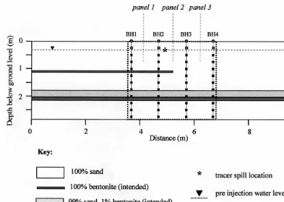
struc-Fig. 1. Cross-section along image plane of intended experimental tank structure; expected deviations are discussed in the text.
ture was not entirely successful as it proved difficult to construct the bentonitersand slurry on top of the powdered bentonite layer without mixing of the two. It is likely that the lower layer is a heterogeneous mixture of the slurry and the bentonite, about 0.3 m thick. In addi-tion, some mixing with the sand above and below both bentonite layers was unavoidable during construction. Consequently, the ‘sand’ between clay layers must be considered to have some variability in terms of porosity, grain size
Ž
and resistivity. Away from the clay layers i.e., above 1.5 m in the region between BH3 and
.
BH4 the sand is considered relatively homoge-neous. The structure is laterally continuous
Žwithin the limits of the construction procedure.
in the plane perpendicular to this cross-section
Žinto the paper . Despite the complications with.
the tank construction, the structure is somewhat representative of an alternating sandrclay
sedi-mentary sequence, in which non-uniform tracer transport can be expected.
The clay layers are high conductivity targets for ERT imaging. Laboratory measurements on sand similar to that placed in the tank gave the resistivity of the sand as 700 V m when satu-rated with tap water of conductivity 5.4 msrm
Žformation factors3.8 . The resistivity of ben-. Ž
tonite slurry was 3 V m average of three repeat
.
measurements ; this slurry was made by mixing
Ž .
bentonite powder with tap water 5.4 msrm . The resistivity of the sandrbentonite mix was not measured but was expected to be signifi-cantly less than the pure sand as small amounts of clay provide surface conduction pathways that reduce bulk resistivity.
For the duration of this experiment the tank was kept in a near saturated state, the water
Ž .
Ž .
surface Fig. 1 . Significant rainfall events
dur-Ž
ing the monitoring period April 1st–April 12th
.
1996 were confined to an event on April 6th, 24 h prior to the termination of tracer injection,
Ž
and an event on April 11th 24 h prior to the
.
collection of the final dataset . As a result of heavy rainfall in the two months prior to this
Ž
experiment the ‘Oregon floods’, February
.
1996 , the tank pore fluid was well flushed with clean water. As minimal electrical contrast be-tween the water added by the two rainfall events and the pore water can be assumed, the primary complication to the data interpretation caused by these events was the increased saturation of the near surface sand. By the end of the experi-ment, the water level was only 0.14 m below
Ž .
the surface a rise of 0.16 m . Given the poros-ity of the sand is 0.38, only 23% of this rise can be associated to the input tracer volume. Tem-perature variations during the monitoring period
Ž .
were moderate 45–658F and not considered to have significantly affected resistivity.
3. Tracer design
An order of magnitude estimate for the grav-ity induced flow of a parcel of fluid of densgrav-ity
Ž y3.
ro kg m through a medium saturated with
Ž
an otherwise stagnant fluid of density ra kg
y3. Ž .
permeability m , gsmagnitude of
gravita-Ž y2.
tional acceleration 9.8 m s and msfluid
Ž y1 y1.
dynamic viscosity 0.001 kg m s . From Eq. 1 a suitable density contrast between the dense tracer and in-situ pore water was calcu-lated. The permeability of the sand was mea-sured as 2=10y11 m2, representative of clean
Ž .
sand Schon, 1996 . From Eq. 1, a tracer of
y1 Ž
concentration 40 g l density contrast 40 kg
y3. Ž .
m results in a downward velocity Vd f0.7 m dayy1. This is an overestimate of the average
Darcy velocity in the tank as the retarding effect of the clay layers is not considered. However,
Ž
given the length of the monitoring period two
.
weeks , a maximum Darcy velocity of 0.7 m dayy1 was considered the correct order of
mag-nitude. Hence, a tracer concentration of 40 g ly1
Ž 3 .
conductivity 8=10 msrm was adopted for this study. Pore water samples obtained follow-ing the termination of the experiment at loca-tions away from the tank center showed in-situ
Ž
fluid conductivity to be 5–8 msrm ;3 orders of magnitude lower than the selected tracer
.
conductivity . This high salinity tracer could represent industrial brine contamination such as
Ž .
that occurring from oil wells Hoekstra, 1998 or serious seawater intrusion into fresh
ground-Ž .
water of coastal aquifers Gondwe, 1991 .
Ž .
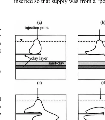
The tracer source shown in Fig. 1 was located to encourage interaction between tracer transport and the known tank structure. A total of 270 of tracer was injected at a rate of 30 mlrmin. The tracer was fed into a glass tube inserted so that supply was from a ‘point’ source
0.3 m below the surface, i.e., into the top of the
Ž .
saturated sediments Fig. 1 . Injection was con-tinuous for 149 h. An idealised schematic of the expected plume evolution is given in Fig. 2.
4. Electrical imaging
As the ERT method is now well described in
Ž
the geophysical literature see for example
.
LaBrecque et al., 1996 only a summary is provided here. Four electrode resistance
mea-Ž
surements the ratio of the voltage between an electrode pair to the current injected between
.
another pair are made for a large number of electrodes placed in boreholes or at the surface. Given these resistance measurements, it is pos-sible to solve numerically for a single resistivity distribution that results in a set of calculated resistance measurements that best represent the measured response. The numerical solution ap-plied here incorporates finite element forward modelling and minimisation of a weighted regu-larised objective function. Full details of the
Ž .
procedure are given in LaBrecque et al. 1996 .
The spatial resolution of electrical imaging is not defined analytically as it is an unknown function of many factors including measure-ment error, electrode geometry, measuremeasure-ment
Ž
schedule number of independent
measure-. Ž
ments and the resistivity distribution Daily and
.
Ramirez, 1995 . During survey design, the spac-ing between electrodes will exert the fundamen-tal control on resolution. Reducing the electrode spacing improves resolution but limits the inves-tigated area, as current is focused in a smaller volume. Consequently, image resolution will decrease away from the electrodes due to the increased distance from the current source. The numerical modelling dictates that the best possi-ble ‘image resolution’ is the size of one element of the finite element mesh. In order to examine the resolution of the final image of resistivity it is possible to determine the resolution matrix, as
Ž .
defined by Menke 1984 .
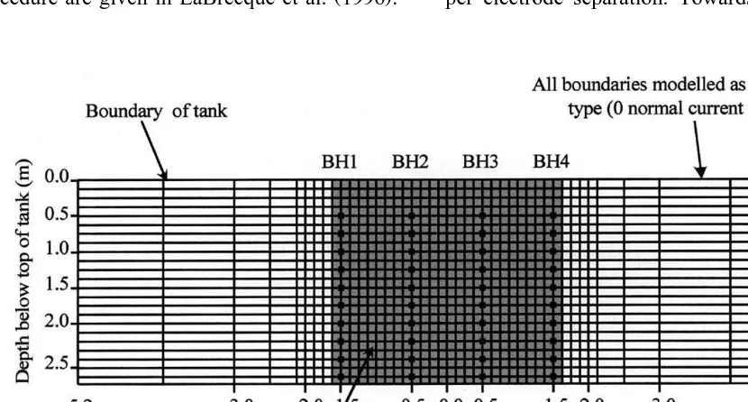
The finite element mesh used in the
resistiv-Ž .
ity modelling LaBrecque et al., 1996 is shown in Fig. 3. The mesh is fine close to the
elec-Ž .
trodes foreground region with two elements per electrode separation. Towards the sides of
the tank the element width increases exponen-tially to reduce computational demand. The electrical insulation provided by the plastic liner was modelled as a Neumann-type boundary
Ž
condition current density perpendicular to the
.
boundary is forced to zero . The modelling ap-plied here assumes a 2-D resistivity distribution. The finite width of the tank in the plane perpen-dicular to the image plane violates this assump-tion. Due to the distance of the electrodes from
Ž
the boundaries of this perpendicular plane 5 m
.
as compared to 1 m between electrode arrays the modelling errors should be small and ac-ceptable given the objectives of this experiment. Numerical methods for imaging 3-D resistivity
Ž
structure have been developed for example,
.
Loke and Barker, 1996 . However, 3-D imaging requires time-consuming acquisition of very large datasets such that its application to imag-ing of tracer tests is currently limited. With future improvements in electrical imaging hard-ware, fast 3-D imaging of tracer tests is likely to be realised. This should significantly increase the value of electrical imaging as geological structure as tracer transport can rarely be two-dimensional.
5. Electrical measurements and noise charac-terisation
Definition of the ‘best’ measurement
sched-Ž
ule a list of four-electrode configurations to be
.
addressed by the resistivity meter remains a
Ž
poorly resolved problem LaBrecque, 1996,
.
pers. comm. . A finite number of independent measurements D can be related to the number of electrodes N,
N N
Ž
y3.
D4s
Ž .
22
Ž . Ž
for a four-electrode dipole–dipole dataset Xu
.
and Noel, 1993 . Circulating measurement schemes have been recommended to guarantee
Ž
completeness of an ERT dataset Xu and Noel,
.
1993 .
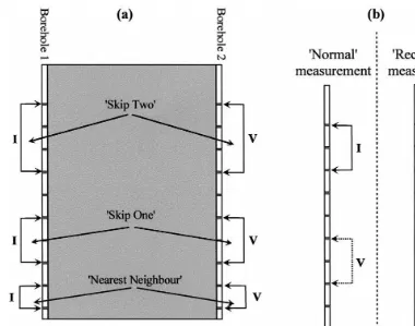
The circulating dipole–dipole schedule
Ž‘nearest neighbour schedule’ , as shown in Fig.. Ž
4a, has been used in the medical field Thomas
.
et al., 1991 and for imaging of soil cores
ŽBinley et al., 1996 . Current is injected be-.
tween two adjacent electrodes and potentials are measured between all remaining adjacent elec-trode pairs. The current elecelec-trodes then circulate by one electrode and all potential pairs are again recorded. One problem with this schedule is that current flow is biased towards the near-borehole region such that resolution at the centre is poor. In addition, the small distance between potential electrodes results in a small voltage signal and a
Ž .
low signal-to-noise ratio SNR . To offset this problem, circulating dipole ‘skip one’ and ‘skip
Ž
two’ measurement schedules were devised Fig.
.
4a . The greater distance between current elec-trodes improves resolution away from the
bore-Ž .
holes as confirmed by synthetic modelling and the increased distance between voltage elec-trodes improves the SNR. Both ‘skip one’ and ‘skip two’ schedules were used to compensate for the loss of some of the independent mea-surements; the circulating dipole schedule con-tains 170 measurements for two boreholes with
Ž .
10 electrodes each Eq. 2, using Ns20 whereas the ‘skip one’ and ‘skip two’ contain only 110 measurements each. Consequently, each between-borehole dataset contained 220 measurements.
Accurate quantification of measurement
er-Ž .
rors noise is crucial to prevent
misinterpreta-Ž .
tion of ERT images LaBrecque et al., 1996 . Measurement noise limits resolution of electri-cal structure. Incorrect noise estimation can
re-Ž
sult in gross smoothing of structure noise
over-. Ž
estimation or artificial image structure noise
.
underestimation . Noise can arise from such
Ž .
factors as 1 poor electrode contact causing systematic errors associated with a particular
Ž .
electrode, 2 random errors associated with the
Ž .
measurement device, and 3 sporadic errors
Ž .
Ž . Ž .
Fig. 4. a Circulating measurement configurations used in electrical imaging. b The ‘‘normal’’ transfer resistance measurement and its reciprocal.
Ž .
Repeatability tests stacking are an obvious measure of noise quantification. An alternative measure is the ‘reciprocal error’, defined as,
esRnyRr
Ž .
3where Rn is the ‘normal’ resistance measure-ment and R is the ‘reciprocal’ resistance mea-r
Ž .
surement Fig. 4b . As exchanging the current electrodes with the potential electrodes should
Ž
not affect the measured resistivity principle of
.
reciprocity , e is a measure of data noise. The reciprocal error can detect errors that may not be apparent from repeatability checks. One ex-ample is the case of bad earth contact at a voltage electrode; the potential between the one connected voltage electrode and the ground on the instrument may be recorded. Interchanging the potential and current electrodes would iden-tify this problem. In this experiment, both
re-peatability errors and reciprocal errors were quantified for each measurement.
The reciprocal errors were used to identify bad measurements and to quantify error parame-ters for the inversion. The inversion uses a simple Gaussian error model in which the
mag-< mag-<
nitude of reciprocal error e increases with the
< <
magnitude of measured resistance R according to,
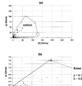
< <esaqb R< <
Ž .
4Parameter a defines the minimum error whereas
< < < <
parameter b defines the increase in e with R . Plots of the reciprocal error against resistance for the background dataset are shown in Fig. 5.
Ž < <
After removal of obvious outliers typically e
< <.
Ž . < < < <
Fig. 5. a Magnitude of reciprocal error e plotted against magnitude of transfer resistance R for all measurements in the
Ž .
background dataset prior to tracer injection. b Remaining errors after removal of obvious outliers; the envelope defines the parameters of the error model.
Electrical measurements were made between
Ž . Ž .
boreholes 1–2 Panel 1 , 2–3 Panel 2 and 3–4
ŽPanel 3 using the lowermost 10 electrodes of. Ž .
each borehole Fig. 1 as the resistive unsatu-rated sand prevented reliable data acquisition using the two uppermost electrodes of each array. A 15-channel data acquisition system
ŽZonge GDP32 , capable of addressing up to 30.
electrodes, was employed. This allowed a
com-Ž
plete three-panel dataset 1320 measurements,
.
including the 660 reciprocals to be collected in approximately 45 min. ERT monitoring of dy-namic hydrological systems requires geophysi-cal equipment that can provide such high data acquisition rates. Prior to tracer injection, a reference ‘background’ dataset was obtained. During the first day of tracer injection,
measure-ments were continually made as fast as the data acquisition hardware would allow. In the fol-lowing period up to two weeks after tracer injection, datasets were collected at least twice daily. Assuming the transport rate to be f0.7 m dayy1
, each image represents a ‘snap-shot’ depiction of the tracer evolution at a particular time.
6. Electrical images
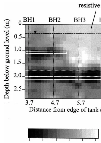
The resistivity image obtained prior to tracer
Ž .
injection ‘background’ is shown in Fig. 6. As expected, two horizontal low resistivity bands correlate with the clay layers. However, the true
Ž . Ž .
Fig. 6. Resistivity structure obtained from inversion of
Ž
electrical measurements prior to tracer injection
back-.
ground dataset .
are not resolved as the maximum resolution
Ž0.125 m as defined by the size of the finite
.
elements is insufficient to resolve this fine structure. In addition, the smoothness con-strained inversion results in a transitional resis-tivity structure in which layer interfaces are not well defined. Consequently, the inversion fits an equivalent layer, which satisfies the data; both
Ž .
the thickness ;0.38 m and the resistivity
Ž6–18 V m of this equivalent layer are overes-.
timates of the true structure. The thickness of
Ž
the lower layer powdered bentonite and slurry
.
layers combined is resolved as a ;0.38 m thick layer in the image; this compares well with the estimated 0.3 m true layer thickness. The resistivity of this lower layer is 5–16 V m; the true resistivity of this layer is not known, but is likely variable due to the mixing between the powdered bentonite and slurry that occurred
during construction. The lowest resistivities probably represent zones of undisturbed ben-tonite.
Ž
Only when away from the sand layers upper
.
right corner of image does the imaged resistiv-ity climb to 1000 V m, comparable with the 800 V m measured for the tap water saturated sand sample in the laboratory. The higher in-situ values probably arise as a result of the flushing of the near surface sand with clean rainwater
Ž .
during February 1996 ‘Oregon floods’ . Be-neath the lower clay layer and between the upper and lower layers, the resistivity is only 100–200 V m, a result of the unavoidable mixing of the sand with the bentonite that oc-curred during array installation. The water table is not resolved in this image. This is primarily due to the reduced resolution near the tank surface, as evident from the diagonal of the
Fig. 7. Resolution matrix for the dataset collected prior to
Ž .
resolution matrix for the three
borehole–bore-Ž .
hole planes Fig. 7 . Values of the resolution matrix range from zero to unity, by definition.
Values close to unity indicate perfect resolution, lower values reveal areas of poorer resolution. The poor resolution above 0.5 m arises as the
Ž .
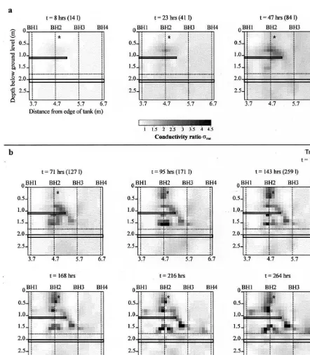
Fig. 8. Images of conductivity ratio at nine times during tracer injection. a Between 8 and 47 h after the start of the tracer
Ž .
first measuring electrode is at 0.5 m, such that the current density in the top 0.5 m is low relative to below 0.5 m. Fig. 5 also shows that, as expected, resolution is greatest close to the boreholes. A second factor preventing the detec-tion of the water table may be the low electrical
Ž .
contrast between fresh-water ;5 msrm satu-rated, and unsatusatu-rated, clean sand.
ERT imaging of tracer transport is best pre-sented using images of conductivity change rel-ative to the pre-tracer condition. Conductivity structure caused by time-static features, such as the sand-clay sequence, is then not apparent in the image, thereby enhancing visualisation of the time varying features. Assuming other
fac-Ž
tors that affect conductivity porosity, saturation
.
and temperature remain constant, images of conductivity change reflect tracer migration alone. In the presentation of image changes, one approach is simply to subtract the pixel conduc-tivity at time t after tracer injection from the pre-injection value. However, as errors are addi-tive when taking the difference of two numbers, the resulting images can be noisy. An alterna-tive is to perform the modelling and inversion on a conductance ratio Crat between two datasets defined as,
Ct
Crats CF
Ž .
5CO
where C is a conductance measurement at timet t, CO is the pre-injection conductance measure-ment and CF is the theoretical conductance for an arbitrary homogeneous conductivity distribu-tion. The output is an image of relative
conduc-Ž .
tivity conductivity ratio srat, in which a value
Ž
of 1 indicates no change between datasets Daily
.
and Owen, 1991 . Values of srat greater than 1 indicate zones of conductivity increase whereas values less than 1 indicate conductivity de-crease. In addition to preventing error propaga-tion, application of Eq. 5 is advantageous as the scaling by CF reduces the complicating effect of departures from a 2-D conductivity
distribu-Ž .
tion, as detailed in Ramirez et al. 1996 .
Images of conductivity ratio at nine times after tracer injection are shown in Fig. 8. In order to enhance the subtle changes that occur in the early stages of injection, the first three images are plotted on a separate scale. The overall picture of tracer transport is as follows: after 23 h accumulation upon the upper clay layer is observed. Transport over the edge of the clay layer is suggested after 47 h and well defined after 95 h. Spreading along both the upper and lower clay layer is apparent after 143 h and somewhat enhanced in the final three datasets. These images are consistent with the order of magnitude prediction of vertical plume transport of 0.7 mrday, as after ts23 h saline water is imaged at 1.0 m. The upper clay layer impedes further vertical transport at this point.
After 71 h, the image indicates evidence for a transport pathway not expected from the
layer-Ž .
ing and the assumed plume evolution Fig. 2 . High srat values are apparent immediately above the lower clayrslurry layer between about
Ž .
4.5 and 5.0 m see also ts95 h . It is likely that, either damage to the upper clay layer occurred in this vicinity, or BH2 acted as a hydraulically conductive flow pathway through the upper layer. The effect of boreholes on subsurface flow structure is a limitation of ERT
Ž
imaging as with any method that involves
inva-.
sion of the subsurface . Conductivity increases immediately above the tracer injection point may represent a localised increase in the groundwater level, although saturation was never observed at the surface. However, as discussed, the sensitivity in the top 0.5 m is poor such that observed changes in this zone are of question-able interpretation. Further discussion of the significance of the observed electrical changes is presented following the discussion of the concept of pixel breakthroughs.
7. Analysis of pixel breakthroughs
attempt to presentrinterpret the data in a man-ner akin to established hydrological methods. ERT images are composed of a large number of pixels that are the elements of the finite element mesh. In this case, each element in the fore-ground region of Fig. 8 is a pixel in the image. Each pixel has a value P that is the ratio of pixel conductivity at time t to initial
conductiv-Ž . Ž .
ity Eq. 5 . Binley et al. 1996 demonstrated how each pixel in a time sequence of electrical images obtained on laboratory soil cores could be interpreted as a ‘breakthrough curve’ of rela-tive tracer concentration. This interpretation
as-Ž . Ž .
sumed 1 full saturation of the pore space, 2 changes in electrical conductivity are only due
Ž .
to changes in fluid conductivity, 3 electrical conductivity is linearly related to salt
concentra-Ž .
tion, and 4 matrix conductivity is small rela-tive to electrolytic conductivity.
In this study, assumptions 1 to 3 can be made if the analysis is performed excluding the upper 0.3 m of unsaturated sand. However, two ben-tonite layers, combined with the relatively low
Ž
fluid conductivity prior to tracer injection 5–8
.
msrm , violate the fourth assumption. In loca-tions close to the bentonite, the relaloca-tionship between fluid and pixel conductivity is influ-enced by the clay content. However, away from the bentonite this relationship will be relatively constant across the tank. Despite this complica-tion caused by the surface conductance close to the bentonite, pixel breakthrough curves of ratio
Ž
conductivity translation to relative fluid
con-.
ductivity not justified should still provide a
Ž . Ž .
qualitative sense of variability in tracer transport
Ž
characteristics breakthrough-recession
be-.
haviour within the tank.
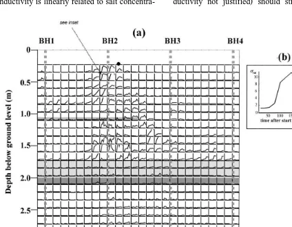
Pixel ‘breakthroughs’ for all elements of the finite element mesh are shown in Fig. 9. Spatial variability in tracer breakthrough-recession be-haviour is apparent and some correspondence with traditional advective-dispersive transport behaviour is observed. Early breakthrough times down to 1.7 m are observed in pixels adjacent to BH2, giving a clear indication of an un-wanted hydraulic pathway through the upper clay layer. Early breakthrough times are also clearly associated with the desired flow pathway over the upper clay layer. The lack of pixel response at between 4.9–5.1 m and 1.25–1.5 m depth testifies to the separation of these two pathways. Pixel response along the top of the upper and lower layers is somewhat consistent with continued plume spreading along these layers.
Fig. 9 also reveals evidence for transport through the lower clayrslurry layer as signifi-cant breakthrough responses are observed be-neath 2.2 m, particularly between BH2 and BH3. Difficulties encountered with the array installation resulted in structural heterogeneity in this layer. Although this could provide verti-cal preferential flow paths, tracer transport along BH2, and perhaps BH3, must also be expected. These pixel responses are not easily defined
Ž .
from the images of conductivity change Fig. 8 . Pixels coincident with the low resistivity
re-Ž .
sponse to the clay layers Fig. 6 show a damped breakthrough relative to breakthroughs observed within the sand. This may in part relate to minimal tracer invasion into the clay containing
Ž
zone both the clay layer and the surrounding sand that was partly mixed with clay during
.
tank construction . However, as discussed, the fluid conductivity–bulk conductivity relation-ship is altered close to the layers as a result of the parallel surface conduction associated with the clay. This is likely the cause of the damped response in some of the pixels immediately above the upper and lower clay layers.
Quantita-tive interpretation of the shape of pixel break-throughs is, hence, complicated. However, the determination of first arrival time seems feasible as picking the first significant increase in con-ductivity is possible from both the sharp re-sponse observed in the sand and the damped response close to the clay. An image of time to first breakthrough is presented in Fig. 10. Such an image perhaps has greater meaning in terms of hydrogeology, relative to an image of con-ductivity change. The image is a rather crude representation of travel time as the sampling interval is coarse, particularly during the later stages of the experiment. However, the image concisely illustrates the two preferential flow pathways identified above.
In-situ pore fluid conductivity was sampled at discrete points following termination of the tracer experiment on April 12th 1996. Sampled
Ž
conductivity varied from 5 msrm the
pre-injec-. 3 Ž
tion value in the sand to 6=10 msrm tracer
3 .
conductivitys8=10 msrm . Sample
loca-Ž .
tions five wells are superimposed on the
im-Ž
age of conductivity ratio for the same day Fig.
.
11 , with values grouped into four categories for ease of presentation. In a general sense, the
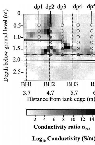
Fig. 11. Sampled fluid conductivity compared to modelled conductivity ratio at 48 locations; well dp6 is shown to illustrate conductivity away from boreholes and tracer.
samples support the distribution of conductivity change obtained from the imaging. Fluid con-ductivity is greatest along the top of the lower clay layer and close to BH2. The location of dp2 was selected to confirm the unwanted flow pathway through the upper clay layer, probably provided by BH2. High fluid conductivity is indeed observed along the length of dp2. For dp4 and dp5, the image pixel values are consis-tent with the samples of fluid conductivity; excluding the lower two samples, pre-injection values of fluid conductivity correlate with pixels showing no conductivity increase. Increased fluid conductivity at the fifth and sixth sample locations for dp6 indicates that tracer transport along the lower clay layer continued outside of the imaged plane.
Closer examination of image pixels at the sample locations reveals some discrepancies.
Considering dp2, the first, second, fourth and
Ž .
fifth from top samples correlate well with sampled fluid conductivity; ratio conductivity is high where sampled fluid conductivity is high, and low where sampled fluid conductivity is low. However, the pixels at the third and sixth sample points correlate poorly with the high fluid conductivity at these locations. This might be the result of the effect of the parallel surface conduction pathway in the presence of high clay content. In such locations, large increases in fluid conductivity may not drastically increase
Ž
bulk conductivity relative to the increase that
.
would be observed in clean sand . A similar lack of correlation between high fluid conduc-tivity and pixel response is observed for the sixth sample in dp4. Along dp1 fluid conductiv-ity samples do not support the elevated conduc-tivity resolved in the pixels above the upper clay layer. However, ratio conductivity is gener-ally lower in a strip centred on dp1, relative to either side.
The observed discrepancies likely in part re-flect the non-unique nature of electrical resistiv-ity imaging. The result from an inversion based on linear least-squares fitting of the data and model roughness is just one of a host of
possi-Ž .
ble image solutions the equivalence problem . In 2-D cross-borehole electrical imaging, the equivalence problem generally does not impede interpretation of overall image structure. How-ever, when performing a detailed analysis of the magnitude of individual pixels, the non-unique nature of the image must always be considered.
8. Discussion
The hydrogeological interpretation of this controlled tracer test identifies the potential value of electrical imaging in groundwater stud-ies. It seems reasonable to consider the image as
Ž .
a set of ‘samplers’ pixels which allow spatial
Ž .
analysis of 1 the distribution of travel times;
Ž .
transport occurs. The fundamental value is the
Ž
very high ‘sampler’ density 598 pixels in this
.
case , relative to that typically obtained with direct, invasive temporal monitoring of fluid conductivity. It is possible that such pixel break-throughs could be applied to formulate a statisti-cal characterisation of variability in transport
Ž
parameters e.g., advective velocity, dispersion
.
coefficient . Such data could be utilised to con-strain stochastically driven solute transport models.
However, the limitations of the method must be recognised. In this particular case, surface conduction effects associated with the two clay layers complicated spatial pixel correlation across the image. As a consequence, the only quantitative interpretation of the pixel break-through curves attempted here was the determi-nation of first arrival times. The second limita-tion, fundamental to any electrical imaging survey, is the non-unique nature of the image solution. Non-uniqueness must be addressed when considering the hydrogeological signifi-cance of changes in individual pixels. Further-more, pixel breakthrough curves are only useful to the extent that the imaging is reliable. This highlights the importance of careful error analy-sis and the removal of bad data prior to inver-sion. Thorough error analysis places additional demands on data acquisition.
The hydrogeological significance of pixel breakthroughs would have been better assessed if fluid conductivity could have been sampled at discrete points during the experiment. Although this was considered, concerns regarding disrup-tion of the ‘natural’ subsurface flow by repeated invasive sampling prevented this approach. Per-manent installation of fluid conductivity sensors prior to electrical imaging would improve future electrical imaging of tracer tests.
As a consequence of the indirect nature of the electrical measurement of fluid conductivity, hydrological interpretation following electrical imaging of a tracer test will be predominantly qualitative. However, for tests in the saturated zone it may be possible to quantify pixel solute
concentration breakthroughs when surface con-duction effects are negligible. This will arise when clay content is insignificant andror fluid conductivity is sufficiently high that electrolytic conduction dominates. Quantitative modelling in terms of advective-dispersive parameters might then be appropriate. However, this condi-tion is not frequently met in the field. The primary hydrological value of electrical imaging is, hence, considered to be the improved spatial coverage of qualitative information that can be related to variations in transport characteristics. Efficient quantification of transport character-istics at a study site could follow from focusing of direct hydrological measurementsrsampling based on transport-induced changes observed in the electrical images. In this manner, a rela-tively small number of direct measurementsr
samples might quantify the primary transport properties at a study site.
Certain problems with interpretation arose as a result of ERT experimental design. The hy-draulic heterogeneity within the tank
signifi-Ž .
cantly differed from that intended Fig. 1 . Swelling of the bentonite upon saturation un-doubtedly caused some mixing between sand and clay. As the nature of this mixing could not be quantified, it reduced the level of control on the tank conditions. The major cause of prob-lems encountered during ERT installation ap-pears to have been a preferential flow pathway close to BH2. The sampled post-experiment fluid distribution supports this conclusion. It is likely that the electrode array itself contributed to the hydraulic conductivity of this flow path. The disruption of the natural flow regime by the emplacement of electrode arrays is a problem general to cross-borehole electrical imaging. Care should be taken to avoidrminimise the hydraulic connections caused by the borehole. In this case, the relatively close proximity of the tracer injection point to BH2 may have encour-aged tracer transport along this borehole. In addition, the electrical imaging indicates some tracer transport through the lower clay layer
tive note, this example illustrates how electrical imaging is capable of defining relatively
com-Ž .
plex flow pathways including unexpected ones in layered media.
A second problem with the ERT experiment design relates to the unsaturated state of the upper 0.4 m prior to tracer injection. As a result of the high contact resistance between electrode
Ž
and dry sand, the top two electrodes at 0 and
.
0.25 m were rendered redundant. The result was poor image resolution in the upper 0.5 m,
Ž .
as revealed by the resolution radius Fig. 7 . Consequently, the location of the water level was not resolved in the imaging, except close to the tracer injection after 95 h of tracer input. Two rainfall events during the period of imag-ing increased the water level but probably had little effect on the fluid conductivity distribu-tion, due to the similar conductivity of the rain water and in-situ tank fluid.
9. Conclusions
In an experimental tank, tracer migration through a synthetic alternating sandrclay se-quence was observed. Images revealed preferen-tial flow through the sand and retardation at the clay layers. Analysis of the 598 pixel break-throughs offered the opportunity to examine the spatial variation in the time-response to tracer transport in a conventional hydrological sense. A crude quantitative assessment of travel times and a qualitative overview of advective-disper-sive transport characteristics were obtained from the breakthrough curves. Unexpected vertical flow paths caused by complications with array installation were identified and supported by post-imaging sampling of fluid conductivity at discrete points within the tank. In particular, natural gravity induced flow was disturbed by the presence of a carefully installed borehole, illustrating how invasive drilling can affect aquifer hydraulic properties.
In this study, tracer transport was modelled in two dimensions: as hydrological processes are
inherently three dimensional, such two-dimen-sional characterisation is not ideal. Computa-tional advances have made three-dimensional electrical imaging possible. New resistivity imaging systems are being marketed that offer rapid data acquisition rates. These systems are ideal for monitoring tracer tests using perma-nent electrode installations. Given continued ad-vances in these two areas, improved resolution of tracer transport from electrical imaging may be anticipated.
Acknowledgements
This work was supported by Ph.D.
stu-Ž
dentship GT4r94r171rL Natural
Environ-.
ment Research Council awarded to the first author. Special thanks are owed to Matt Perrot
ŽCenter for Groundwater Research, Oregon
.
Graduate Institute of Science and Technology for assistance with fieldwork.
References
Archie, G.E., 1942. The electrical resistivity log as an aid in determining some reservoir characteristics. Trans. Am. Inst. Min. Metall. Pet. Eng. 146, 54–62.
Binley, A., Henry-Poulter, S., Shaw, B., 1996. Examina-tion of solute transport in an undisturbed soil column using electrical resistance tomography. Water Resour. Res. 32, 763–769.
Brewster, M.L., Annan, A.P., Greenhouse, J.P., Kueper, B.H., Olhoeft, G.R., Redman, J.D., Sander, K.A., 1995. Observed migration of a controlled DNAPL release by geophysical methods. Ground Water 33, 977–987. Buselli, G., Barber, C., Davis, G.B., Salama, R.B., 1990.
Detection of groundwater contamination near waste disposal sites with transient electromagnetic and
electri-Ž .
cal methods. In: Ward, S.H. Ed. , Investigations in Geophysics No. 5: Geotechnical and Environmental Geophysics. Environmental and Groundwater Vol. 2 Society of Exploration Geophysicists, Oklahoma, pp. 27–39.
Butler, D.K., Llopis, J.L., 1990. Assessment of anomalous
Ž .
Daily, W., Owen, E., 1991. Cross-borehole resistivity to-mography. Geophysics 56, 1228–1235.
Daily, W., Ramirez, A., Johnson, R., 1998. Electrical impedance tomography of a perchloroethylene release.
Ž .
J. Environ. Eng. Geophys. 2 3 , 189–202.
Daily, W., Ramirez, A., LaBrecque, D., Barber, W., 1995. Electrical resistance tomography experiments at the Oregon Graduate Institute. J. Appl. Geophys. 33, 227– 237.
Daily, W., Ramirez, A., LaBrecque, D., Nitao, J., 1992. Electrical resistivity tomography of vadose water move-ment. Water Resour. Res. 28, 1429–1442.
Gondwe, E., 1991. Saline water intrusion in southeast Tanzania. Geoexploration 27, 25–34.
Hoekstra, P., 1998. Geophysical surveys for mapping brine contamination resulting from oil and gas production. In: Symposium on the Application of Geophysics to
Engi-Ž .
neering and Environmental Problems SAGEEP , March 22–26, Chicago, IL. pp. 197–204.
Johansson, S., Dahlin, T., 1996. Seepage monitoring in an earth embankment dam by repeated resistivity measure-ments. Eur. J. Environ. Eng. Geophys. 1, 229–247. LaBrecque, D.J., Miletto, M., Daily, W., Ramirez, A.,
Owen, E., 1996. The effects of noise on Occam’s inversion of resistivity tomography data. Geophysics 61, 538–548.
Loke, M.H., Barker, R.D., 1996. Practical techniques for 3D resistivity surveys and data inversion. Geophys. Prospect. 44, 499–523.
Menke, W., 1984. Geophysical Data Analysis: Discrete Inverse Theory. Academic Press.
Osiensky, J.L., Donaldson, P.R., 1995. Electrical flow
through an aquifer for contaminant source leak detec-tion and delineadetec-tion of plume evoludetec-tion. J. Hydrol. 169, 243–263.
Ramirez, A., Daily, W., Binley, A.M., LaBrecque, A., Roelant, D., 1996. Detection of leaks in underground storage tanks using electrical resistance methods. J. Environ. Eng. Geophys. 1, 189–203.
Schon, J.H., 1996. Physical properties of rocks: fundamen-tals and principles of petrophysics, Handbook of Geo-physical Exploration; Seismic Exploration. Pergamon. Thomas, D.C., McArdle, F.J., Rogers, V.E., Beard, R.W.,
Brown, B.H., 1991. Local blood volume changes in women with pelvic congestion measured by applied
Ž .
potential tomography. Clin. Sci. 81 3 , 401–404. Vanhala, H., 1996. Monitoring the integrity of liner
con-struction using induced polarisation. In: Proceedings of the Symposium on the Application of Geophysics to Environmental and Engineering Problems, April 28th– May 2nd, 1996, Keystone, CO. pp. 1017–1026. White, P.A., 1988. Measurement of ground-water
parame-ters using salt-water injection and surface resistivity. Ground Water 26, 179–186.
White, P.A., 1994. Electrode arrays for measuring ground-water flow direction and velocity. Geophysics 59, 192– 201.
Wilt, M.J., Alumbaugh, D.L., Morrison, H.F., Becker, A., Lee, K.H., Deszcz-pan, M., 1995. Crosswell electro-magnetic tomography: system design considerations and field results. Geophysics 60, 871–885.