T H E J O U R N A L O F H U M A N R E S O U R C E S • 47 • 1
Male Earnings
Methods and Evidence
Robert A. Moffitt
Peter Gottschalk
A B S T R A C T
We estimate the trend in the transitory variance of male earnings in the United States using the Michigan Panel Study of Income Dynamics from 1970 to 2004. Using an error components model and simpler but only ap-proximate methods, we find that the transitory variance started to increase in the early 1970s, continued to increase through the mid-1980s, and then remained at this new higher level through the 1990s and beyond. Thus the increase mostly occurred about 30 years ago. Its increase accounts for be-tween 31 and 49 percent of the total rise in cross-sectional variance, de-pending on the time period.
I. Introduction
A substantial literature has accumulated on trends in various mea-sures of instability in individual earnings and family income in the United States over the last 30 or so years, with many studies finding increases in instability (Gott-schalk and Moffitt 1994; Moffitt and Gott(Gott-schalk 1995; Dynarski and Gruber 1997; Cameron and Tracy 1998; Haider 2001; Hyslop 2001; Stevens 2001; Moffitt and Gottschalk 2002; Dynan et al. 2008; Keys 2008; Jensen and Shore 2010; Shin and Solon 2010). Increases also have been found in Canada (Baker and Solon 2003; Beach et al. 2003; Beach et al. 2010; Ostrovsky 2010) and the United Kingdom (Dickens 2000). Interest in trends in instability, particularly instability that comes
Robert A. Moffitt is a Professor of Economics at Johns Hopkins University. Peter Gottschalk is a Re-search Professor of Economics at Boston College. The authors would like to thank two referees at this journal and the participants at many seminars and conferences for comments, Joe Tracy and John Abowd for discussant comments, and Tom DeLeire and Gary Solon for helpful conversations. Outstand-ing research assistance was provided by Yonatan Ben-Shalom, Kai Liu, Shannon Phillips, and Sisi Zhang. The data used in this article can be obtained beginning June 2012 through May 2015 from Robert A. Moffitt, Department of Economics, Johns Hopkins University, Baltimore, Maryland 21218, moffitt@jhu.edu.
[Submitted August 2008; accepted March 2011]
Moffitt and Gottschalk 205
from an increase in the transitory variance of earnings, has arisen for many reasons. One reason is that Friedman (1957) argued in his classic treatise that transitory fluctuations should have little or no impact on consumption. A massive literature over the subsequent five decades has followed, showing that consumption and saving respond differently to permanent and transitory changes in income (Attanasio and Weber 2010). A recent contribution by Blundell, Pistaferri, and Preston (2008), for example, argues that considerable consumption smoothing takes place in response to transitory shocks but much less for permanent shocks. A second, more normative reason for interest in transitory variance is that shocks which cannot be smoothed generally impose welfare losses and, given the evidence that transitory fluctuations are more easily smoothed than permanent shocks, welfare losses are presumably smaller, the greater relative importance of transitory shocks compared to permanent ones. Third, and relatedly, many students of inequality have long noted that transitory shocks have little impact on the inequality of lifetime incomes, whereas permanent shocks do. This has normative implications for inequality (Atkinson and Bourguig-non 1982; Cowell 2000; Gottschalk and Spolaore 2002; Sen 2000). Fourth, a liter-ature which assumes that social welfare depends on whether it is possible for indi-viduals to change their rank in the income distribution over their lifetimes argues that increases in the variance of permanent shocks, which move individuals farther apart in the distribution and hence makes changes in rank less likely are social-welfare-detracting. In contrast, transitory changes in income, which mix up the dis-tribution and result in more changes in rank are social-welfare-improving (Shorrocks 1978; Gottschalk and Spolaore 2002).
A purely labor economics motivation for an interest in distinguishing permanent from transitory shocks relates to the well-known increase in cross-sectional inequal-ity (Katz and Autor 1999). By definition, an increase in cross-sectional inequalinequal-ity has to arise from an increase in permanent shocks, transitory shocks, or both. The literature has put forth explanations for this trend in inequality (for example, skill-biased technical change), which all assume that permanent shocks have generated the cross-sectional increase, yet, statistically, a rising cross-sectional variance could also result from an increase in the transitory variance. Explanations for rising tran-sitory variance are likely to be quite different. For example, the increase in the transitory variance could have been caused by an increase in product or labor market competitiveness, a decline in regulation and administered prices, a decline in union strength, increases in temporary work or contracting-out or self-employment, and similar factors. In addition, insofar as transitory fluctuations are more easily insured against than permanent fluctuations, as just noted, the welfare losses from increases in cross-sectional inequality might be smaller than would otherwise be supposed if transitory fluctuations have been an important source of the increase in cross-sec-tional inequality.
transitory variation. But we also use two simpler methods, one an extension of the method originally suggested by Gottschalk and Moffitt (1994) and the other a new nonparametric method that provides consistent estimates of the transitory variance while making weak assumptions about the structure of the earnings process. These two methods relax some of the strong parametric assumptions made in the error components model but at the cost of providing only approximate estimates. All three methods show rising transitory variances from the 1970s to the 1980s and a leveling off in the 1990s. Some ambiguity attaches to the precise dates at which the variance rises, and at which it levels off, as a result of cyclical events—which have a signifi-cant impact on transitory variances—that occur around the major turning points.
The first section briefly gives the intuition for how trends in transitory variances are identified with a panel data set. The next section describes the data set we construct and the third section lays out our methods and results. We then provide a section that compares our results to others in the literature and provides potential explanations for differences in findings. A brief summary concludes.
II. Identification of Trends in Transitory Variances
The intuition for identification of trends in a transitory variance can be seen from the canonical error components model with permanent and transitory components:
y ⳱Ⳮ
(1) it i it
whereyit is log earnings or residual log earnings for individualiat age t,itis a time-invariant, permanent individual component, andit is a transitory component. The typical assumptions are that E()⳱E( )⳱E( )⳱0,Var()⳱2 and
i it i it i
. Identification and estimation of this basic random effects model has
2
Var( )⳱ it
been known since the 1960s. However, typically these models assume E( )⳱
it i but this has been shown not to hold in most earnings applications. When 0 for t⬆
it does not hold, identification is less obvious. Carroll (1992) was, to our knowledge, the first to point out explicitly that identification in this case can be obtained from “long” autocovariances. The covariance of yit between periodsapart is
2
Cov(y ,y )⳱ ⳭCov( , )
(2) it i,tⳮ it i,tⳮ
and hence2 is identified fromCov(y ,y ), which is observed in the data,
pro- it i,tⳮ
vided thatCov( , )⳱0.1ButCov( , )⳱0is essentially the definition of it i,tⳮ it i,tⳮ
a transitory component in the first place, because this covariance represents the persistence of such a component—that is, whether a transitory shock at timetⳮis
still present, even in reduced magnitude, by timet. If the definition of a transitory component is something that eventually goes away, the permanent variance must be identified at sufficiently high values of(more on this below).
Moffitt and Gottschalk 207
Once the permanent variance is identified, the transitory variance is identified as the residual:
2 2
⳱Var(y )ⳮ
(3) it
becauseVar(yit)is observed in the data. This exercise can be conducted in different calendar periods, thereby revealing whether transitory variances are changing.
This method of identification of permanent and transitory variances from the long autocovariances ofyitis employed in the richer error components model as well as the nonparametric method described below. The data requirements are therefore for a sufficiently long panel which allows not only calculation of variances but also long autocovariances, and for different periods of calendar time.
III. Data
The Michigan Panel Study on Income Dynamics (PSID) satisfies these requirements, for it covers a long calendar time period (1968–2005 at the time this analysis was conducted) and, because it is a panel, we can compute autocovar-iances of earnings between periods quite far apart. We use the data from interview
year 1971 through interview year 2005.2 Earnings are collected for the previous
year, so our data cover the calendar years 1970 to 2004. The PSID skipped inter-views every other year starting in interview year 1998, so our last five observations are for earnings years 1996, 1998, 2000, 2002, and 2004. The sample is restricted to male heads of households. Females are excluded in order to reduce the selection effects of the increasing number of females participating in the labor market. Only heads are included since the PSID earnings questions we use are only asked of heads of household. We take any year in which these male heads were between the ages of 30 and 59, not a student, and had positive annual wage and salary income and positive annual weeks of work. We include men in every year in which they appear in the data and satisfy these requirements. We therefore work with an unbalanced sample because of aging into and out of the sample in different years, attrition, and movements in and out of employment. Fitzgerald, Gottschalk, and Moffitt (1998) have found that attrition in the PSID has had little effect on its cross-sectional representativeness, although less is known about the effect of attrition on autoco-variances. Measurement error in earnings reports is another potential problem when using survey data to estimate covariance matrices. However, Pischke (1995) has shown that measurement error in the PSID has little effect on earnings covariances and Gottschalk and Huynh (2010) show that this is a result of the non-classical structure of measurement error in earnings found in many surveys.3We exclude men
2. We do not use earnings reported in 1969 or 1970 since wage and salary earnings, which is what we use, are reported only in bracketed form in those years.
in all PSID oversamples (SEO, Latino). All earnings are put into 1996 CPI-U-RS dollars. The resulting data set has 2,883 men and 31,054 person-year observations, for an average of 10.8 year-observations per person. Means of the key variables are shown in Appendix Table A1.
Rather than form a variance-autocovariance matrix directly from these earnings observations, we work with residuals from regressions of log earnings on education, race, a polynomial in age, and interactions among these variables, all estimated separately by calendar year. Our analysis, therefore, estimates the transitory com-ponent of the within group variance of log earnings. We use these residuals to form a variance-autocovariance matrix indexed by year, age, and lag length. Thus, a typ-ical element consists of the covariance between residual log earnings of men at ages a anda’ between years tandt’. Because of sample size limitations, however, we cannot construct such covariances by single years of age. Instead, we group the observations into three age groups—30–39, 40–49, and 50–59—and then construct the variances for each age group in each year, as well as the autocovariances for each group at all possible lags back to 1970 or age 20, whichever comes first. We then compute the covariance between the residual log earnings of the group in the given year and each lagged year, using the individuals who are in common in the two years (when constructing these covariances, we trim the top and bottom one percent of the residuals within age-education-year cells to eliminate outliers and top-coded observations4). The resulting autocovariance matrix represents every
individ-ual variance and covariance between every pair of years only once, and stratifies by age so that life cycle changes in the variances of permanent and transitory earnings can be estimated (the human capital literature has shown that there are life cycle patterns in earnings variances). The covariance matrix has 1,197 elements over all years, ages, and lag lengths. A few specimen elements are illustrated in Appendix Table A2.
After presenting our main results, we will report the results of sensitivity tests to a number of the more important of these data construction decisions.
IV. Models and Results
We present results on trends in transitory variances from three mod-els: a parametric error components model; an approximate nonparametric imple-mentation of that model; and an even simpler method used originally by Gottschalk and Moffitt (1994) which also only approximates the variances of interest.
A. Error Components Model
We first formulate an error components (EC) model of life cycle earnings dynamics process in the absence of calendar time shifts. There is a large literature on the
Moffitt and Gottschalk 209
formulation of such models (Hause 1977; Lillard and Willis 1978; Lillard and Weiss 1979; Hause 1980; MaCurdy 1982; Abowd and Card 1989; Baker 1997; Geweke and Keane 2000; Meghir and Pistaferri 2004; Guvenen 2009; see MaCurdy 2007 for a review). These models have suggested that the permanent component is not fixed over the life cycle but evolves, typically with variances and covariances rising with age. This pattern can be captured by a random walk or random growth process in the permanent effect. The literature has also shown that the transitory error is serially correlated, usually by a low-order autoregressive moving-average (ARMA) process. Our model contains all these features:
y ⳱ Ⳮ
4 again posits a permanent-transitory model but with an age-varying permanent effect (ia). The latter evolves over the life cycle from a random growth factor ( )␦i
which allows each individual to have a permanently higher or lower growth rate than that of other individuals, and from a random walk factor (ia) that arrives randomly but is a permanent shock in the sense that it does not fade out over time as the individual ages. The transitory error evolves according to a ARMA(1,1) pro-cess typically found in the literature, with the underlying transitory shock (ia) fading out at rate but deviating from that smooth fade-out rate by in the next period (the MA(1) parameterimproves the fit of the lag process significantly). Our tests also show, consistent with other findings in the literature, that higher order ARMA parameters are not statistically significant. We assume all forcing errors to be i.i.d.
except ia, whose variance we assume to vary with age because transitory shocks
are likely to be greater at younger ages. We allow i0 and␦i to be correlated in light of the Mincerian theory that they should be negatively related (those who have higher initial investments in human capital will start off low but rise at a faster rate). Hence
2 2 2 2 2 2 2
E(␦)⳱ , E( )⳱ , E( )⳱ Ⳮ a, E( )⳱ and E( ␦)⳱ .
i ␦ ia ia 0 1a i0 0 i0 i ␦
An important point to note is that, in this more realistic model, compared to the simple canonical model outlined previously, transitory shocks never completely fade out because of the AR(1) process, which implies that they fade out only asymptot-ically. Consequently, the variance of the permanent effect can never be exactly iden-tified by the long autocovariances, as we argued it should be, above. The permanent variance (and hence the transitory variance as well) is therefore identified by ex-trapolation of the AR(1) curve to infinity. However, provided thatis not too high, the covariance will fall to a low value over the 34 years of our data, reducing the extrapolation problem to some degree.5
With this identification condition satisfied, the parameters of the model can be identified for a single cohort. Determining whether there are calendar time shifts can therefore be identified from changes in parameters across multiple cohorts, for that allows a comparison of variances and covariances at the same point in the life cycle but at different calendar time periods. Although all the parameters of the model could potentially shift with calendar time, for reasons of convenience and on the basis of past work testing for calendar-time shifts in the other parameters (Moffitt and Gottschalk 1995), we allow calendar time shifts in only two places in the model, in the permanent component and the forcing transitory component:
y ⳱␣ Ⳮ
where t is calendar time. The parameter ␣t alters the variance of the permanent
effect, which is now ␣2Var( ). This formulation coincides with an interpretation
t ia
ofiaas a flow of human capital services and␣tas its time-varying price, consistent with the literature on changes in the returns to skill. We force it to be the same for all ages although this could be relaxed. The parametertlikewise allows calendar time shifts in the variance of the transitory component, which is now2Var( ).
t ia
The introduction of time-varying parameters introduces a problem of left-censor-ing because those parameters cannot be identified prior to 1970 yet their evolution prior to that year affects variances and covariances after 1970. To address this issue,
we introduce an additional parameter ␥ which allows the transitory variances in
1970 to deviate from what they would be if⳱1fort⬍1970, with␥⳱0implying t
no deviation. The details are given in Appendix 2.
For any set of values of the parameters, the model in Equations 7–9 generates a set of predicted variances and covariances in each year and for each age and lag length, and therefore a predicted value for each of the 1,197 elements of our data covariance matrix. We estimate the parameters by minimizing the sum of squared deviations between the observed elements and elements predicted by the model, using an identity weighting matrix and computing robust standard errors. The formal
statement of the model and estimating procedure appears in Appendix 2.6
The estimates of the model parameters are given in Appendix Table A3. The transitory component is significantly serially correlated both through the AR(1) and MA(1) component, implying, as discussed before, that long autocovariances are needed to identify the model, and the variances of the random walk and random growth errors in the permanent component are both statistically significant; and the initial permanent and transitory components are indeed negatively correlated. How-ever, our main interest is in the estimates of␣tandtwhich are shown graphically
6. We estimate the model in levels rather than differences. The individual effecti0does not cancel out
in differences in our model because of the␣t. In addition, the covariance matrix of the differences of␥iat
Moffitt and Gottschalk 211
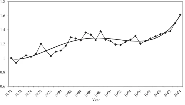
Figure 1
Error Components (EC) Model Estimates of Alpha
Notes: In this and subsequent figures, the four PSID non-interview years are interpolated from the two adjacent points. The trend line is fit from a fifth order polynomial.
in Figures 1 and 2 along with smoothed trend lines (both are normalized to one in 1970).7Figure 1 shows that the permanent variance rose starting in the early 1970s,
continued to rise through to the mid-1980s, leveled off or declined slightly from then through the mid-1990s, and then started rising again in the mid-1990s. This pattern in within group permanent variance is roughly consistent with rises in the return to education and other indicators of skill differentials shown in the cross-sectional literature on inequality trends. This pattern reflects, as has already been emphasized and as will be shown explicitly below, trends in the long autocovariances in the data.8
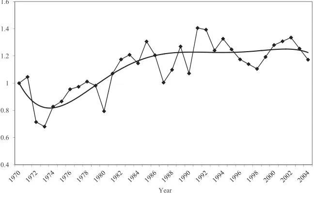
Of more direct interest to our focus on the transitory variance of earnings is Figure 2, which shows the estimated values of t along with a trend line. The transitory variance rose sharply starting in the early 1970s, and then continued to rise, albeit at a slower rate, until the mid-1980s, after which time it has remained flat, although with major fluctuations (that is, it remained flat on average, as shown by the smoothed line). As we will show momentarily, recessions in the early 1980s, early 1990s, and early 2000s caused jumps in the transitory variance which prevent us
Figure 2
Error Components (EC) Model Estimates of Beta
from being precise about the exact dates at which some of the trends stopped rising or leveled off. Nevertheless, our general answer to the question we posed in the introduction is: the transitory variance of male earnings started to increase in the early 1970s, continued to rise through the mid-1980s, and then stabilized at a new higher level.
The evolution over time in the variance of the transitory component, whose
for-mula is shown in Equation 9, is not quite the same as that of t since the latter
feeds into the transitory variance in future periods, and similarly for the permanent variance. Drawing the implications of our estimated parameters for the variances of
and requires applying the formulas in Appendix 2. Figure 3 shows the
␣ t ia iat
Moffitt and Gottschalk 213
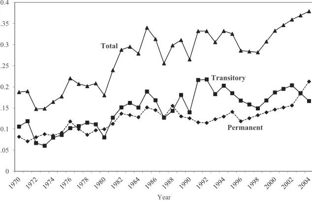
Figure 3
Fitted Permanent, Transitory, and Total Variances of Log Earnings Residuals, Age 30–59 (EC Model)
or no growth in the permanent variance. However, as Figure 3 shows, the permanent variance resumed its upward trend in the mid-1990s and continued through 2004.
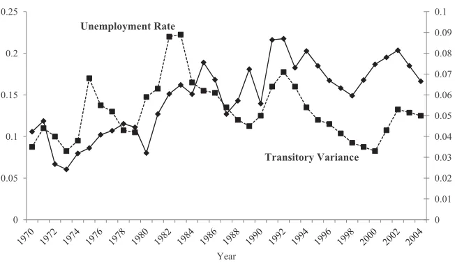
Much of the fluctuation in the transitory variance is business-cycle related. Figure 4 shows the same transitory variance but plotted along with the national unemploy-ment rate for men 20 and over. The variance is clearly positively correlated with the unemployment rate, albeit with something of a lag in the first half of the period. The recession of the early 1980s appears to have been responsible for some of the transitory variance increase in the early 1980s, but the variance never returned to its pre-1980s levels in the late 1980s, when the unemployment had fallen. The transitory variance increase in the early 1990s appears to also have been partly business-cycle related, its decrease from the early 1990s to 1997 appears to be related to the decline in the unemployment rate (although, once again, it did not return to its former level), and the increase in the variance in the early 2000s corresponds to the recession in that period. Thus the fluctuations after approximately 1990 appear to be cyclically induced. However, the average level of the transitory variance during the decade of the 1990s was above its average level in the 1980s, even the late 1980s. Thus our evidence also suggests, albeit with considerable uncertainty as to the exact timing, that the transitory variance in the 1990s may have been slightly higher than in the 1980s. Nevertheless, even if true, the size of the increase was much less than the size of the increase from the 1970s to the 1980s.
spec-Figure 4
Fitted Transitory Variances of Log Earnings Residuals, Age 30–59 (EC Model) and Unemployment Rate
Note: Male Unemployment Rate Age 20 and over
ifications of the permanent and transitory components than assumed in our para-metric model. We consider two simpler methods to address this question.
B. Approximate Nonparametric Method
One approach is to follow the simple model described in Section I by using the long autocovariances to estimate the variance of the permanent effect and by then sub-tracting that value from the total variance to obtain an estimate of the transitory variance. Figure 5 shows the variance of log annual earnings residuals in each year for those 30–39, for illustration, along with the autocovariances between those re-siduals in each year and those in years six and ten years previous, which might be considered to be sufficiently long that the transitory shocks are no longer correlated. The figure shows this not to be the case for the lag-six autocovariance, which is above that at lag ten, indicating that the autocovariance is still falling between six and ten years previous (the lag-ten autocovariance may, of course, not be long enough either). Taking the difference between the upper line for the variance and the line for the lag-ten autocovariance results in an estimate of the transitory variance which is plotted in Figure 6 (it necessarily starts in 1980, since a ten-year lag is needed to compute it). These estimates show an increase in the transitory variance in the early 1980s followed by a reversal, and fluctuations but no clear trend over the entire period. This is quite different than the pattern shown in the EC model.
Moffitt and Gottschalk 215
Figure 5
Variances and Autocovariances, Age 30–59
model of the age-evolution of the permanent effect shown in Equation 4ⳮ6 with
its random walk and random growth specifications implies that the relevant long autocovariance is no longer equal to the variance of the permanent component, as it was in the simple canonical model.9The second is that the method does not work
well when ␣tis evolving over the period covered by the long autocovariance, for
in that case the autocovariance ofyiatis
Cov(y ,y )⳱␣ ␣ Cov( , )
(10) iat i,aⳮ,tⳮ t tⳮ ia i,aⳮ
and therefore the long autocovariance will not equal ␣2Cov( , )because␣
t ia i,aⳮ t
is changing over time. For example, Cov(yiat,yi,aⳮ,tⳮ) will rise at a faster rate than ␣tis rising if recent lagged ␣tⳮ have also been rising. Specifically, the rise
in ␣t in the 1970s and early 1980s shown in Figure 1 will cause later
to rise “too much,” leading to an excess decline in the transitory Cov(yiat,yi,aⳮ,tⳮ)
variance because it is obtained as the residual from subtracting Cov(yiat,yi,aⳮ,tⳮ) from the total variance.10
Nevertheless, Equation 10 forms a basis for a better method of applying the idea of using the long autocovariances to obtain an estimate of the permanent variance,
9. See Appendix Equations (2–15) and (2–16): the autocovariance in (2–16) equals the permanent variance in (2–15) only if the random walk and random growth terms do not appear.
0.35
0.3
0.25
0.2
0.15
0.1
0.05
0
Figure 6
Implied Transitory Variances of Log Earnings Residuals Using, 10-Lag Autocovariance, Age 30–39
which we term the approximate nonparametric (NP) method. Taking the logs of Equation 10, we have
log
[
Cov(y ,y )]
⳱log␣Ⳮlog␣ Ⳮlog[
Cov( , )]
(11) iat i,aⳮ,tⳮ t tⳮ ia i,aⳮ
⳱log␣Ⳮlog␣ Ⳮf(a,) t tⳮ
an equation which should hold, again, if the lag order is high enough that the
transitory errors are no longer correlated. Equation 11 can be estimated by OLS using year dummies to capture the log␣t and log␣tⳮ and if (say) a polynomial approximation in a and is used to approximate log
[
Cov(ia,i,aⳮ)]
nonpara-metrically. We denote that approximation asf(a,). The variance of the permanent component is then estimated by using the fitted Equation 11, evaluated at⳱0.11The influence of the laggedlog␣tⳮon the autocovariance is captured by the lagged year dummies. This method is nonparametric because it imposes no parametric model on the evolution of the permanent effect—random walk, random growth, or something else—with that evolution approximated by an arbitrary function of age and lag length; and because it imposes no parametric model on the evolution of the transitory component, except to assume that that component is not correlated after
Moffitt and Gottschalk 217
Figure 7
Approximate Nonparmetric (NP) Estimate of Transitory Variance of Log Earnings Residuals
Notes: Averaged over all ages
a sufficient length of time. But it is only approximate because the effects of past transitory shocks are never exactly zero because of the presence of the AR(1) pro-cess.
C. Window Averaging Method
An even simpler method introduced by Gottschalk and Moffitt (1994) and applied in some subsequent studies is to estimate the permanent and transitory variances with standard random-effects formulas within moving calendar time windows of
fixed length, which we denote the window averaging (WA) method.12To estimate
the transitory variance in yeart, the 2wⳭ1 residuals in the calendar time window
[tⳮw, tⳭw] are averaged for each individualito obtain an estimate of the
individ-ual’s permanent component. The difference between the residual for each individual in each year and the individual’s average residual constitutes an estimate of the transitory component. Then the textbook formulas for the random effects model are used to compute the variances of the two components.13Repeating this process for
each successive yeartin the data—with a shift in the window each time—a trend
in the estimated transitory variance is generated.
If the window is limited to two periods, the variance of transitory earnings com-puted in this way is closely related to the variance of the change in earnings
(y ⳮy ) between the periods. This can be seen by recognizing that when
iat i,aⳮ1,tⳮ1
the window is limited to two periods, a transitory component calculated as the de-viation of earnings in periodtfrom the average earnings over periodstandtⳮ1 is
equal to one-half times the change in earnings between the periods. In this case the variance of transitory earnings is equal to one-quarter of the variance of the change in earnings. When the window is longer than two periods, this equivalence no longer holds.
The WA method produces consistent estimates of the transitory variance under the canonical model described in Section I because that model corresponds to the textbook random effects model whose estimator we use. However, in more general models the residuals used in the computation are not quite the right ones if the permanent and transitory components follow the more complex, serially-correlated process in our EC model. The method is also not well-suited to detecting exact turning points in trends because it averages over years. Nevertheless, it is an ap-proximation which has the virtue of simplicity and transparency whose defects may not be quantitatively important.
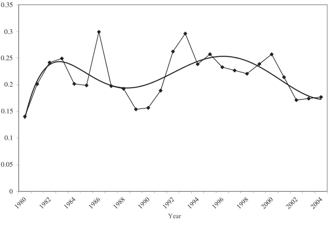
Figure 8 shows the WA estimates using a nine-year window. Thus the earliest date is 1974 and the latest is 2000 because of the requirement of four years of data on either side of the year in question. The results are quite similar to those from the EC model shown in Figure 4 and the NP model shown in Figure 7, rising from the 1970s to the 1980s and leveling off around 1990, a bit later than in the other methods but not drastically so. The variance turns up at the end, for the year 2000 window, but Figure 4 and Figure 7 show that this upturn is followed by a downturn in the
12. In a prior version of this paper, and in some other work, this method has been referred to as the “BPEA” method.
Moffitt and Gottschalk 219
Figure 8
Window Averaging (WA) Estimate of Transitory Variance, 9-year Window
years which follow. Because of the averaging that is part of this method, the series is much smoother than that of the other methods.
D. Sensitivity Tests
We conduct sensitivity tests to several of the more important data construction de-cisions we have made in this study. All sensitivity tests are conducted using the simplest method, the WA method, and all results are shown graphically in Appendix 3. We examine the effect on the results from (1) using residuals that do not take out age and education effects, (2) restricting the sample to those who worked 48 or more weeks per year, (3) trimming the data to lesser or greater degrees than in our base case, and (4) including nonworkers.
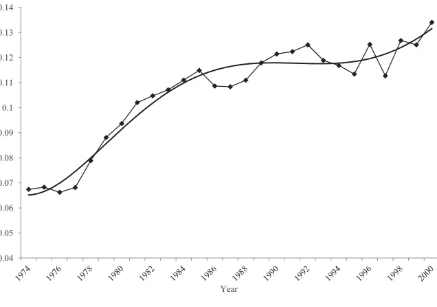
It is of interest to know whether the increased transitory variance has been a result of increased transitory variance of wage rates or labor supply. A full investigation of this issue is beyond the scope of this paper, but a simple method often used to isolate something close to a wage rate is to select workers who work full year. Figure 3–2 shows the pattern of transitory variances based on a sample of men who worked at least 48 weeks in the year. The same pattern of sharply increased variances from the 1970s to the 1980s as in Figure 8 is exhibited, although the uptick in the late 1990s and early 2000s in that Figure does not appear, suggesting that the var-iance of weeks worked may have increased in that period. However, as we noted previously, our EC and NP methods imply that variances turned down subsequent to 2000, and it could easily be that the early-2000s recession generated a short-term increase in the variance of weeks worked. Further investigation of the issue is war-ranted.
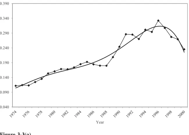
Our main results are based on data in which the top and bottom one percent of earnings residuals within age-education-year cells are deleted, both to eliminate top-coded observations and to eliminate earnings observations with low and high values in general, which can have a disproportionate effect on logarithmic transformations. Figure 3-3(a) shows estimates when no trimming is done. Variances are much higher in this case (compare its vertical axis with that of Figure 8) but the same upward trend through the early 1990s is present, though the jump in the variance in the early 1990s is much larger, which may be a result of changes in PSID procedures in that period which we discuss further below. The transitory variance does turn down at the end, but this may also be traceable to the high rates of variances in the early 1990s. Figure 3-3(b) shows trends when five percent of each tail is trimmed and shows that the upward trend from the 1970s to 1980s continues to be robust to this additional trimming. However, there is a stronger increase in the late 1990s and early 2000s in this case, which must mean that the 95th to 99th percentiles or the 1st to 5th percentiles moderated the increase in the variance.
To include nonworkers, we must modify our method because log earnings cannot be used. We include nonworkers by changing from calculations of variances to calculations of percentile points, using percentile points of the non-logarithmic earn-ings distribution. To accomplish this, we select the log earnearn-ings residuals we have used thus far for each individual in each year and calculate the anti-logarithm of
each.14 Following the WA method, we then compute the average of these
trans-formed residuals for each individual in a nine-year window over working years only and, finally, we compute, for each year, an individual’s ratio of his transformed residual in that year to his mean. This ratio signifies the fraction by which (non-logged) earnings in the year is in excess of, or below, his mean over all years, and thus measures a relative transitory component. In years in which an individual is a nonworker, this fraction is zero by definition. We then compute the percentile points of the distribution of these fractions in each year.
Moffitt and Gottschalk 221
Figure 3-4(a) shows percentile point trends excluding nonworkers to determine if this method yields the same result as our variance calculations above. All four per-centile points in the figure show a marked spreading-out of the distribution from the 1970s to the 1980s. Thus the increase in variance we have found previously is not a result of a change in only one part of the distribution, but is rather widely spread across the entire distribution. The percentile points are stable through the late 1990s but, again consistent with the variance calculations, a slight spreading out of the distribution occurs at both high and low percentile points starting in the late 1990s. Figure 3-4(b) shows the trends including nonworkers (between 10 percent and 14 percent of these prime-age men were nonworkers, depending on the year). The upper three percentile point patterns are virtually the same as in Figure 3-4(a) but the 10th percentile point pattern shows a sharper rate of increased dispersion from the 1970s to the 1980s but then a narrowing in the 1990s, ending up in 2000 only slightly below its initial 1974 value. The inclusion of nonworkers, it should be noted, should increase cross-sectional dispersion but has no necessary implication for trends in the transitory variance, which will depend on the degree to which nonworking status has become more persistent rather than more unstable. If the rate of nonwork in-creases but becomes more persistent, this will not increase the transitory variance. The pattern in the figure suggests that nonworking did, in fact, become more per-sistent in the 1990s for the lower tail of the distribution, leading to a decline in transitory dispersion in those years.
V. Differences Across Studies
There have been several other studies in the literature which separate permanent from transitory components and have estimated whether the male earnings variance of the transitory component has increased with calendar time in the United States (Gottschalk and Moffitt 1994; Moffitt and Gottschalk 1995; Haider 2001; Stevens 2001; Hyslop 2001; Moffitt and Gottschalk 2002; Gottschalk and Moffitt 2006; Keys 2008; Jensen and Shore 2010). These studies all find increases in the transitory variance over time, particularly from the 1970s to mid-1980s. Those later studies which examined the period after the mid-1980s report different results, some finding no trend in the 1990s while others finding some decrease and others finding an increase. Moffitt and Gottschalk (2002), for example, find a decrease from the early 1990s to 1996, but our current results show that decrease to be temporary and probably a result of cyclical factors. Also, Gottschalk and Moffitt (2006) found a larger increase in the 1990s than we find in this study (as noted above, we find a small increase in that period), but this is a result of improvements in the model specification.15 Overall, however, this literature reinforces the view that transitory
variance increases were greater in the 1970s and 1980s than anything in the 1990s.
Another strand in the literature does not attempt to separate permanent from tran-sitory variances but instead focuses on trends in the variance of one-year or two-year changes in male annual earnings, often termed ‘volatility’. While most of these studies find, like us for transitory variances, increases in volatility in the 1970s and early 1980s (Dynarski and Gruber 1997; Cameron and Tracy 1998; Dynan et al. 2008; Shin and Solon 2010), the two studies which had data through the late 1990s and early 2000s showed an additional significant increase in that period (Dynan et al. 2008; Shin and Solon 2010), which we do not find despite using the same data; and one study found no increase at all in earlier periods, in contrast to our findings (U.S. Congressional Budget Office 2007; Dahl et al. 2010).16These differences must
be traced either to differences in the measures—transitory variances versus volatil-ity—or to differences in data.
Regarding differences in the measures, the most obvious difference is that the volatility measure includes changes in the instability of permanent earnings as well as transitory earnings. The authors of these studies argue that there is considerable interest among policy-makers and others in volatility per se regardless of the per-manent-transitory decomposition of such changes. We do not disagree with that view but believe that the classically-defined decomposition into these two components is of additional interest for the reasons noted in the Introduction. The inclusion of permanent earnings in the volatility measure explains one of the two differences in findings we noted above, namely, why Dynan et al. (2008) and Shin and Solon (2010) find significant increases in volatility in the late 1990s and early 2000s whereas our EC model finds no increase in the transitory variance in that period (aside from cycle). Since we find that there was a marked increase in the permanent variance in that period, as shown in Figure 1, a measure which aggregates increasing permanent variances and stable transitory variances should show an increase. Our data, indeed, show such an aggregate increase in the variance of two-year changes in log residual earnings in the last years of the data (see Appendix Figure 3–5; this result also holds for log earnings itself rather than residuals).17
As for differences with these two studies in treatment of the PSID data, while there are differences in age ranges, variable definitions, and related decisions that we would expect to have only minor effects, two differences could be important.18
One is that both studies included nonworkers in some of their volatility measures whereas we exclude nonworkers from our main transitory variance calculations. However, as we noted above in our discussion of sensitivity tests, including non-workers does not change our results (Shin and Solon (2010) also calculated their estimates with and without nonworkers and found little difference). The other
dif-16. In addition, Shin and Solon (2010) find a slight decline in the 1990s rather than a flattening out or slight increase, as we find. This is a less important difference, but we remark on it below.
17. This also explains the difference in trends in the 1990s between our study and that of Shin and Solon (2010), who find a decline in volatility over that period instead of a flattening out, for we find that the permanent variance declined in that period (see Figures 1 and 3 above).
Moffitt and Gottschalk 223
ference is that, as Dynan et al. (2008) emphasize, the introduction of Computer Assisted Telephone Interviewing in the PSID in 1992 and a shift to new data pro-cessing software in 1993 may also have led to a spurious one time shift in measures of instability. Dynan et al. (2008) find an unusually large increase in the number of individuals who change from positive earnings to zero earnings from 1991 to 1992, even though hours worked were reported in the latter year; they find that excluding those with zero earnings but positive hours leads to a reduction in estimated volatility over those years. More generally, they find an increase in the number of low earners in this period relative to previous years of the PSID. Once again, however, our results do not appear to be sensitive to this issue as far as we can determine, even though complete certainty about the effect of this change is not known. For example, we include in our sample only men with both positive earnings and positive weeks worked in our sample, thereby accomplishing the restriction imposed by Dynan et al. In addition, as we already noted, the inclusion of nonworkers does not affect our results when we use percentile point measures of transitory dispersion. Finally, as our discussion of sensitivity to trimming above indicated, our one-percent trim at both tails does indeed remove the major jump in transitory variance in the 1991– 1993 period, and further trimming does not have much effect on reducing the size of the modest jump that remains.
As for the difference in findings with the U.S. Congressional Budget Office (2007) (CBO) and Dahl et al. (2010), who find no upward trend (if not a downward one) in volatility, we should immediately note that the latter study restricted its analysis to years 1985 and after on the grounds that the Social Security earnings data prior to those years—which were used in the earlier CBO report—had been discovered suspect and were no longer sufficiently trustworthy to use. However, our results and theirs for the years 1985 and after differ very little, for both Dahl et al. (2010) and we find no long-term trend in volatility or transitory variance after that year. Our
results show that the major upward trend was completed by the mid-1980s.19
Of course, there is a major difference in the data used, for these studies use administrative earnings reports from the Social Security Administration whereas we use household survey data, which may contain response error. However, the two data sets also differ in their sample populations—the Social Security data contain non-heads and the PSID data only cover heads, and neither data set can replicate the other’s sample—and the Social Security data have somewhat different coverage than the PSID. Further, earnings recorded on Social Security records have some errors, and there are some items likely to be reported in a survey that are excluded
from the relevant line on W-2 forms (Abowd and Stinson 2010). In addition, the simple presumption that the Social Security data contain less response error is not consistent with the finding in several studies that those data show greater cross-sectional dispersion than do survey data, not less (Abowd and Stinson 2010; Gott-schalk and Huynh 2010), suggesting that there may be other differences in either the populations or the earnings measures than simple reporting error. The reasons for differences in the data sets certainly deserve further investigation.
VI. Summary
We have provided new estimates of the trend in the transitory vari-ance of male earnings in the United States using the Michigan Panel Study of Income Dynamics through 2004. Our study uses the classical definition of a transitory com-ponent that fades out over time and eventually disappears altogether, as distinct from a permanent component that never goes away. Using both an explicit error com-ponents model as well as two simpler but more approximate methods, we find that the transitory variance increased substantially in the 1970s and early 1980s and then remained at this new higher level through 2004. We also find a strong cyclical component to the transitory variance which induced major jumps in the variance during the recessions of the early 1980s, early 1990s, and early 2000s. Our conclu-sion that the transitory variance was stable, net of cycle, after the mid-1980s results from our interpretation that the changes in the transitory variance were cyclical and that there was no trend after that time, although it is possible that that transitory variance was slightly higher than it was previously. The trend increase in the tran-sitory variance accounts for about half of the increase in cross-sectional inequality through the late 1980s but only for about a third through 2004 because the permanent variance has been rising markedly since the mid-1990s. Since other research has shown that a significant proportion of transitory shocks can be smoothed, these findings imply that the welfare implications of the rise in cross-sectional inequality experienced in the United States are less serious than they might otherwise have been thought to be. Put differently, the rise in cross-sectional inequality corresponds to a smaller increase in lifetime inequality.
These results are robust both to the methodology used and to data construction decisions related to outliers and trimming, inclusion of non-workers, and related issues. We have also reconciled our results with most other studies, although there is some uncertainty whether findings from the PSID give the same results as those from administrative data drawn from Social Security earnings files which deserves further research.
Moffitt and Gottschalk 225
Annual real earnings $43,514.00 $26,516.00 $615.00 $525,015.00
Log annual real
Means taken over all person-year observations (NT⳱30,424).
Means taken after 1 percent trimming within age-education-year cells for paired observations. a. Multiplied by 10,000; residual mean is close to zero.
Appendix Table A2
Specimen Elements of the Covariance Matrix: Year 1974
Year Age Lag Year Lag Age Covariance
1974 35 1970 31 0.0783
Ages in the table denote midpoints of a ten-year group (35⳱30–39, 34⳱29–38, etc.). Covariance element values are after 1 percent trimming.
Appendix Table A3
Estimates of the Error Components Model
Appendix 2
with the following normalizations, variance assumptions, and initial conditions:
␣ ⳱1, ⳱1
and witha⳱1 defined as age 20. For the left-censored (1970) observations, define
a70as the individual’s age in 1970. Those witha70⬎1 are left-censored. We define
the variance of the transitory component in 1970 for these left-censored observations in the following way (the variance of the permanent component does not require knowledge of␣tprior to 1970):
⳱ Ⳮ Ⳮ
Equation 2–10 is the ARMA(1,1) expression for the 1970 transitory component. Only the first and third terms are prior to 1970 and hence only they must be ap-proximated. Equation 2–12 gives the formula for the variance of the transitory
com-ponent for someone who is age a70 in 1970 and whose transitory component has
followed its age evolution from agea⳱1 to that age witht⳱1 in all those years.
Equation 2–11 allows that age profile of transitory variances to be modified by the parameter␥, and it is assume that the deviation is a function of age—the lower the age, the fewer years prior to 1970 have occurred, and hence the smaller the expected
deviation. We denote the expression in (2–11) as g(a70) for use in the formulas
below.
An alternative treatment of the left-censored observations would simply allow the
Moffitt and Gottschalk 229
whose parameters would be estimated. However, this approach would result in a misspecification in the present case because it would make all succeeding transitory variances a function of calendar time (we do not demonstrate this for brevity). As
a result, even in a model with ␣⳱⳱1, the model would predict calendar time
t t
evolution of the variances and covariances. Thus true calendar time shifts after 1970 would be confounded with distance from the left-censoring point, generating incor-rect estimates of␣tandt(see MaCurdy 2007, pp. 4094–4098 for a related discus-sion).
The unknown parameters in the model are ␣,,, , ,␥,2 ,2,2, and .
t t 0 1 0 ␦ ␦
They generate the following variances and covariances for all years, ages, and lag lengths.
If a70⬍1 (nonleft-censored):
2 2
If a70⬎1 (left-censored):
2 2
the log earnings residuals for individualifor age-year “locations”jandk, and where m⳱1, . . . ,Mindexes the moments generated by the product of residuals at all loca-tionsjandk. In our case,M⳱1,197. Write the model in generalized form as
s ⳱f(,j,k)Ⳮε i⳱1, . . . ,N, m⳱1, . . . ,M
whereis aLx1 vector of parameters. Then the set ofMequations in 2-23 consti-tutes a SUR system whose efficient estimation requires an initial consistent estimate
of the covariance matrix of the εim. However, following the findings and
recom-mendations of Altonji and Segal (1996) on bias in estimating covariance structures
of this type, we employ the identity matrix for the estimation. Hence we choose
to minimize the sum of squared residuals:
N M
2
min
[
s ⳮf(,j,k)]
(2-24)
兺 兺
im i⳱1m⳱1
or, equivalently, sincefis not a function ofi,
M
2
min
[
s¯ ⳮf(,j,k)]
(2-25)
兺
im m⳱1
wheres¯im is the mean (overi) ofsim(in other words, a covariance).
To obtain standard errors, we apply the extension of Eicker-White methods in the manner suggested by Chamberlain (1984), using the residuals from (2-24), each of which we denoteeim. Let⍀be theMxMcovariance matrix of theeim, each element
of which is estimated by:20
N
1 ˆ
⳱ e e
(2-26) mm⬘
兺
im im⬘Ni⳱1
DefineDas theNMxNMcovariance matrix of individual residuals which is a block
diagonal matrix with the matrix⍀on the diagonals. Then
ⳮ1 ⳮ1
ˆ
Cov()⳱(GG) G⬘DG(GG)
(2-27)
whereGis theNMxL matrix of gradientsf(,j,k).
Moffitt and Gottschalk 231
Appendix 3
Figure 3-1
Window Averaging (WA) Estimate of Transitory Variance of Log Earnings Residuals, 9Year Window, Year Residuals Only
Figure 3-2
Figure 3-3(a)
(WA) Estimate of Transitory Variance, No Trainning
Figure 3-3(b)
Moffitt and Gottschalk 233
Figure 3-4(a)
Percentile Points of the Relative Transitory Component Distribution, excluding Nonworkers
Figure 3-4(b)
Figure 3-5
Variance of Two-Year Difference in Log Residual Male Annual Earnings
References
Abowd, John, and David Card. 1989. “On the Covariance Structure of Earnings and Hours Changes.”Econometrica57(2):411–45.
Abowd, John, and Martha Stinson. 2010. “Estimating Measurement Error in SIPP Annual Job Earnings: A Comparison of Census Survey and SSA Administrative Data.”
Unpublished manuscript. Ithaca, NY and Washington, D.C.: Cornell University and U. S. Census Bureau.
Altonji, Joseph, and Lewis Segal. 1996. “Small Sample Bias in GMM Estimation of Covariance Structures.”Journal of Business and Economic Statistics14(3):353–66. Atkinson, Anthony, and Francois Bourguignon. 1982. “The Comparison of Multidimensional
Distributions of Economic Status.”Review of Economic Studies49(2):183–201. Attanasio, Orazio, and Guglielmo Weber. 2010. “Consumption and Saving: Models of
Intertemporal Allocation and Their Implications for Public Policy.”Journal of Economic Literature48(3):693–751.
Baker, Michael. 1997. “Growth-Rate Heterogeneity and the Covariance Structure of Life-Cycle Earnings.”Journal of Labor Economics15(2):338–75.
Baker, Michael, and Gary Solon. 2003. “Earnings Dynamics and Inequality Among Canadian Men, 1967–1992: Evidence from Longitudinal Income Tax Records.”Journal of Labor Economics21(2):289–322.
Moffitt and Gottschalk 235
———. 2010. “Long-Run Inequality and Short-Run Instability of Men’s and Women’s Earnings in Canada.”Review of Income and Wealth56(3):572–96.
Blundell, Richard, Luigi Pistaferri, and Ian Preston. 2008. “Consumption Inequality and Partial Insurance.”American Economic Review98(5):1887–1921.
Cameron, Stephen, and Joseph Tracy. 1998. “Earnings Variability in the United States: An Examination Using Matched-CPS Data.” Unpublished manuscript. New York: Columbia University and Federal Reserve Bank of New York.
Carroll, Christopher. 1992. “The Buffer-Stock Theory of Saving: Some Macroeconomic Evidence.”Brookings Papers on Economic Activity2:61–135.
Chamberlain, Gary. 1984. “Panel Data.” InHandbook of Econometrics, Vol. 2, eds. Zvi Griliches and Michael Intriligator, 1247–1318. Amsterdam: North-Holland.
Cowell, F. 2000. “Measurement of Inequality.” InHandbook of Income Distribution, eds. Anthony Atkinson and Francois Bourguignon, Vol. I, 87–166. Amsterdam and New York: Elsevier North Holland.
Dahl, Molly, Thomas DeLeire, and Jonathan Schwabish. 2010. “Estimates of Year-to-Year Variability in Worker Earnings and in Household Incomes from Administrative, Survey, and Matched Data.” Washington: Congressional Budget Office. Unpublished.
Dickens, Richard. 2000. “The Evolution of Individual Male Earnings in Great Britain: 1975–95.”Economic Journal110(460):27–49.
Dynan, Karen, Douglas Elmendorf, and Daniel Sichel. 2008. “The Evolution of Household Income Volatility.” Unpublished manuscript. Washington: Brookings Institution. Dynarski, Susan and Jonathan Gruber. 1997. “Can Families Smooth Variable Earnings?”
Brookings Papers on Economic Activity1:229–303.
Fitzgerald, John, Peter Gottschalk, and Robert Moffitt. 1998. “An Analysis of Sample Attrition in Panel Data: The Michigan Panel Study of Income Dynamics.”Journal of Human Resources33 (2): 251–99.
Friedman, Milton. 1957.A Theory of the Consumption Function. Princeton: Princeton University Press.
Geweke, John and Michael Keane. 2000. “An Empirical Analysis of Earnings Dynamics Among Men in the PSID: 1968–1989.”Journal of Econometrics96(2):293–356. Gottschalk, Peter, and Minh Huynh. 2010. “Are Earnings Inequality and Mobility
Overstated? The Impact of Non-classical Measurement Error.”Review of Economics and Statistics92(2):302–15.
Gottschalk, Peter, and Robert Moffitt. 1994. “The Growth of Earnings Instability in the U.S. Labor Market.”Brookings Papers on Economic Activity2:217–72.
———. 2006. “Trends in Earnings Volatility in the U.S.: 1970–2002.” Paper presented at the Meetings of the American Economic Association, January 2007.
Gottschalk, Peter, and Enrico Spolaore. 2002. “On the Evaluation of Economic Mobility.” Review of Economic Studies69(1):191–208.
Guvenen, Fatih. 2009. “An Empirical Investigation of Labor Income Processes.”Review of Economic Dynamics12(1):58–79.
Haider, Steven. 2001. “Earnings Instability and Earnings Inequality of Males in the United States, 1967–1991.”Journal of Labor Economics19(4):799–836.
Hause, John. 1977. “The Covariance Structure of Earnings and the On-the-Job Training Hypothesis.”Annals of Economic and Social Measurement6(4):335–65.
———. 1980. “The Fine Structure of Earnings and the On-the-Job Training Hypothesis.” Econometrica48(4):1013–1029.
Hyslop, Dean. 2001. “Rising U.S. Earnings Inequality and Family Labor Supply: The Covariance Structure of Intrafamily Earnings.”American Economic Review91(4):755–77. Jensen, Shane, and Stephen Shore. 2010. “Changes in the Distribution of Income Volatility.”
Katz, Lawrence, and David Autor. 1999. “Changes in the Wage Structure and Earnings Inequality.” InHandbook of Labor Economics, Vol. 3A, ed. Orley Ashenfelter and David Card, 1463–1555. Amsterdam and New York: Elsevier North-Holland.
Keys, Benjamin. 2008. “Trends in Income and Consumption Volatility, 1970–2000.” In Income Volatility and Food Assistance in the United States, ed. D. Jolliffe and J. Ziliak, 11–34. Kalamazoo, Michigan: W.E. Upjohn.
Lillard, Lee, and Yoram Weiss. 1979. “Components of Variation in Panel Earnings Data: American Scientists, 1960–1970.”Econometrica47(2):437–54.
Lillard, Lee, and Robert Willis. 1978. “Dynamic Aspects of Earnings Mobility.” Econometrica46(5):985–1012.
MaCurdy, Thomas. 1982. “The Use of Time Series Processes to Model the Error Structure of Earnings in a Longitudinal Data Analysis.”Journal of Econometrics18(1):83–114. ———. 2007. “A Practitioner’s Approach to Estimating Intertemporal Relationships Using
Longitudinal Data: Lessons from Applications in Wage Dynamics.” InHandbook of Econometrics,Vol. 6A, Part 1, ed. James Heckman and Edward Leamer, 4057–167. Amsterdam: Elsevier.
Meghir, Costas, and Luigi Pistaferri. 2004. “Income Variance Dynamics and Heterogeneity.” Econometrica72(1):1–32.
Moffitt, Robert, and Peter Gottschalk. 1995. “Trends in the Covariance Structure of Earnings in the U.S.: 1969–1987.” Unpublished Manuscript. Reprinted inJournal of Economic Inequality. Forthcoming
———. 2002. “Trends in the Transitory Variance of Earnings in the United States.” Economic Journal112(478): C68-C73.
Ostrovsky, Yuri. 2010. “Long-Run Earnings Inequality and Earnings Instability Among Canadian Men Revisited, 1985–2005.”The B.E. Journal of Economic Analysis and Policy 10(1): Article 20:1–32.
Pischke, S. 1995. “Measurement Error and Earnings Dynamics: Some Evidence from the PSID Validation Study.” Journal of Business and Economic Statistics13(3):305–14. Sen, A. 2000. “Social Justice and the Distribution of Income.” InHandbook of Income
Distribution, ed. Anthony Atkinson and Francois Bourguignon, Vol. I, 59–85. Amsterdam and New York: Elsevier North Holland.
Shin, Donggyun, and Gary Solon. 2010. “Trends in Men’s Earnings Volatility: What Does the Panel Study of Income Dynamics Show?” East Lansing, Michigan: Michigan State University. Unpublished.
Shorrocks, Anthony. 1978. “The Measurement of Mobility.”Econometrica46(5):1013–24. Stevens, Anne. 2001. “Changes in Earnings Instability and Job Loss.”Industrial and Labor
Relations Review55(1):60–78.