Full Terms & Conditions of access and use can be found at
http://www.tandfonline.com/action/journalInformation?journalCode=ubes20
Download by: [Universitas Maritim Raja Ali Haji] Date: 11 January 2016, At: 19:14
Journal of Business & Economic Statistics
ISSN: 0735-0015 (Print) 1537-2707 (Online) Journal homepage: http://www.tandfonline.com/loi/ubes20
Comment
Peter Reinhard Hansen & Allan Timmermann
To cite this article: Peter Reinhard Hansen & Allan Timmermann (2015) Comment, Journal of Business & Economic Statistics, 33:1, 17-21, DOI: 10.1080/07350015.2014.983601
To link to this article: http://dx.doi.org/10.1080/07350015.2014.983601
Published online: 26 Jan 2015.
Submit your article to this journal
Article views: 126
View related articles
handle these and other interesting extensions. This fact suggests that much work remains to be done for econometricians going forward.
REFERENCES
Baumeister, C., and Kilian, L. (2012), “Real-Time Forecasts of the Real Price of Oil,” Journal of Business and Economic Statistics, 30, 326– 336. [13]
Baumeister, C., Kilian, L., and Lee, T. K. (2014), “Are There Gains From Pooling Real-Time Oil Price Forecasts?”Energy Economics, 46, S33–S43. [15]
Clark, T. E., and McCracken, M. W. (2012), “In-Sample Tests of Predictive Ability: A New Approach,”Journal of Econometrics, 170, 1–14. [14,15] Clark, T. E., and West, K. W. (2007), “Approximately Normal Tests for Equal
Predictive Accuracy in Nested Models,” Journal of Econometrics, 138, 291–311. [14]
Inoue, A., and Kilian, L. (2004), “Bagging Time Series Models,” CEPR Dis-cussion Paper No. 4333. [13,14,15]
Mark, N. C. (1995), “Exchange Rates and Fundamentals: Evidence on Long-Horizon Predictability,”American Economic Review, 85, 201–218. [13]
Comment
Peter Reinhard H
ANSENDepartment of Economics, European University Institute, 50134 Florence, Italy and CREATES, Aarhus University, DK-8210 Aarhus, Denmark ([email protected])
Allan T
IMMERMANNRady School of Management, UCSD, La Jolla, CA 92093 and CREATES, Aarhus University, DK-8210 Aarhus, Denmark ([email protected])
1. INTRODUCTION
The Diebold-Mariano (1995) test has played an impor-tant role in the annals of forecast evaluation. Its simplicity— essentially amounting to computing a robustt-statistic—and its generality—applying to a wide class of loss functions—made it an instant success among applied forecasters. The arrival of the test was itself perfectly timed as it anticipated, and undoubtedly spurred, a surge in studies interested in formally comparing the predictive accuracy of competing models.1
Had the Diebold-Mariano (DM) test only been applicable to comparisons of judgmental forecasts such as those provided in surveys, its empirical success would have been limited given the paucity of such data. However, the use of the DM test to sit-uations where forecasters generate pseudo out-of-sample fore-casts, that is, simulate how forecasts could have been generated in “real time,” has been the most fertile ground for the test. In fact, horse races between user-generated predictions in which different models are estimated recursively over time, are now perhaps the most popular application of forecast comparisons.
While it is difficult to formalize the steps leading to a sequence of judgmental forecasts, much more is known about model-generated forecasts. Articles such as West (1996), McCracken (2007), and Clark and McCracken (2001, 2005) took advantage of this knowledge to analyze the effect of re-cursive parameter estimation on inference about the parameters of the underlying forecasting models in the case of nonnested models (West 1996), nested models under homoscedasticity (McCracken 2007) and nested models with heteroscedastic
1Prior to the DM test, a number of authors considered tests of forecast
encom-passing, that is, the dominance of one forecast by another; see, for example, Granger and Newbold (1977) and Chong and Hendry (1986).
multi-period forecasts (Clark and McCracken2005). These pa-pers show that the nature of the learning process, that is, the use of fixed, rolling, or expanding estimation windows, matters to the critical values of the test statistic when the null of equal predictive accuracy is evaluated at the probability limits of the models being compared. Giacomini and White (2006) devel-oped methods that can be applied when the effect of estimation error has not died out, for example, due to the use of a rolling estimation window.
Other literature, including studies by White (2000), Ro-mano and Wolf (2005), and Hansen (2005) considers forecast evaluation in the presence of a multitude of models, addressing the question of whether the best single model—or, in the case of Romano and Wolf, a range of models—is capable of beat-ing a prespecified benchmark. These studies also build on the Diebold-Mariano article insofar as they base inference on the distribution of loss differentials.
Our discussion here will focus on the ability of out-of-sample forecasting tests to safeguard against data mining. Specifically, we discuss the extent to which out-of-sample tests are less sen-sitive to mining over model specifications than in-sample tests. In our view this has been and remains a key motivation for focusing on out-of-sample tests of predictive accuracy.
© 2015American Statistical Association
Journal of Business & Economic Statistics
January 2015, Vol. 33, No. 1 DOI:10.1080/07350015.2014.983601
Color versions of one or more of the figures in the article can be
found online atwww.tandfonline.com/r/jbes.
2. OUT-OF-SAMPLE TESTS AS A SAFEGUARD AGAINST DATA MINING
The key advantage of out-of-sample comparisons of predic-tive accuracy emerges, in our view, from its roots in the over-fitting problem. Complex models are better able to fit a given dataset than simpler models with fewer parameters. However, the reverse tends to be true out-of-sample, unless the larger model is superior not only in a population sense–that is, when evaluated at the probability limit of the parameters–but also dominate by a sufficiently large margin to make up for the larger impact that estimation error has on such models.
A finding that a relatively complex model produces a smaller mean squared prediction error (MSPE) than a simpler benchmark need not be impressive if the result is based on an in-sample comparison. In fact, if several models have been esti-mated it is quite likely that one of them results in a substantially smaller MSPE than that of a simpler benchmark. This holds even if the benchmark model is true. For out-of-sample tests the reverse holds: the simpler model has the edge unless the larger model is truly better in population. It is far less likely that the larger model outperforms the smaller model by pure chance in an out-of-sample analysis. As we shall see, in fact it requires far more mining over model specifications in out-of-sample experiments for there to be a sizeable chance of outperforming the benchmark by a “statistically significant” margin.
To illustrate this important difference between in-sample and out-of-sample forecasting performance, consider the simple re-gression model residual sum of squares (RSS) is
RSSin=Y′(In−XX′)Y =ε′(In−XX′)ε=ε′ε−ε′XX′ε. (2) Suppose instead thatβhas been estimated from an independent sample ofβ. Consequently, from (2) the in-sample overfit is given by
Tin=RSS∗−RSSin=ε′XX′ε∼χk2. (4)
From (3) the corresponding out-of-sample overfit statistic is
Tout=RSS∗−RSSout= −ε˜′XX′ε˜+2ε′XX′ε.˜ (5)
Note that the first term isminusaχ2
k-variable while the second term has mean zero sinceεand ˜εare independent. Therefore,
while the estimated model (over-) fits the in-sample data better than the true model, the reverse holds out-of-sample.2
This aspect of model comparison carries over to a situation with multiple models. To illustrate this point, consider a sit-uation where K regressors are available and we estimate all possible sub-models with exactlykregressors so that the model complexity is fixed. Suppose that the MSPE of each of these models is compared to the true model for whichβ=0. Then
Tmaxin = max
j∈KCkT
in
j , (6)
measures how much the best-performing model improves the in-sample RSS relatively to the benchmark. Here,KCkdenotes the number of different models arising from “Kchoosek” re-gressors. The equivalent out-of-sample statistic is
Tmaxout = max j∈KCk
Tjout. (7)
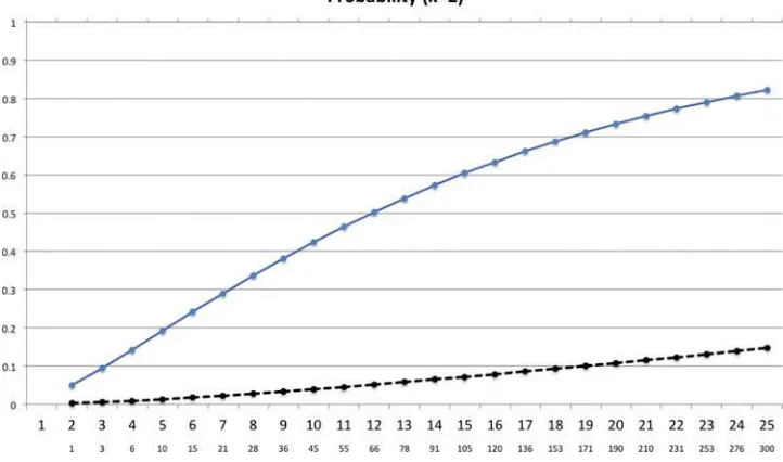
For example, we might be interested in computing the proba-bility that the MSPE of one of the estimated models is less than RSS—for some constant. Not surprisingly, this probability is much smaller for out-of-sample forecast comparisons than for in-sample comparisons. Figures1–4 displays these proba-bilities as a function ofKandk, for the case where the constant,
k, is (arbitrarily) chosen to be the 5% critical value of aχk2 -distribution. This choice ofk is such that the probability of finding a rejection is 5% withk=K. The results fork=1,2,3,
and 4 are displayed in separate figures. Each figure hasKalong thex-axis.Kwhich determines the number of regression mod-els (K choose k) to be estimated and the latter is shown on the secondary (lower)x-axis. The graphs are based on 100,000 simulations and a design whereX′X
=IK andY ∼N(0, In) withn=50 sample observations.
Figures1–4reveal a substantial difference between the effect of this type of mining over models on the in-sample and out-of-sample results. In-out-of-sample (upper line), the probability of finding a model that beats the benchmark by more thank increases very quickly as the size of the pool of possible regressors,K, used in the search increases. By design, the size of the test is 5% only whenk=K, that is, at the initial point of the in-sample graph. However, in each graph the rejection rate then increases to more than 70% whenK=25.
Out-of-sample the picture is very different. The MSPE of the estimated model tends to be worse than that of the true model. Consequently, the probability that the estimated model beats the benchmark by more thankis very small. In fact, it takes quite a bit of mining over specifications to reach even the 5% rejection rate, and the larger iskthe less likely it is to find out-of-sample rejections. For instance, for a regression model with
k=4 regressors it takes a pool ofK =20 regressors for there
the be a 5% chance of beating the benchmark by4 =9.49 or
more. In other words, what can be achieved in-sample, with a single model with four explanatory variables, takes 4845 models sample. This is part of the reason that out-of-sample evidence is more credible than in-out-of-sample evidence; it
2Note that E(Tin−Tout)=2k; this observation motivated the penalty term in Akaike’s information criterion. After applying this penalty term to a model’s in-sample performance it is less likely that the estimated model “outperforms” the true model in-sample.
Figure 1. The figure shows the probability that maxj∈KCkTj> k, that is, the probability that one of more models outperform the benchmark
bykor more, as a function ofK, the total number of (orthogonal) predictors. The secondaryx-axis shows the number of distinct regression
models. The figure assumesk=1.
is far more impressive for a relatively complex model to out-perform a simpler benchmark out-of-sample than in-sample. Attributing such superior performance to mining across model specifications is a less convincing explanation out-of-sample, than it is in-sample.
While out-of-sample tests of predictive accuracy can help safeguard against the worst excesses of in-sample data mining, such tests clearly raise other issues. First, the conclusion that out-of-sample tests safeguard against mining over models hinges on the assumption that the test statistic is compared against standard critical values, precisely as is the case for the Diebold-Mariano statistic. If, instead, larger models are “compensated”
for their complexity, as advocated by Clark and West (2007), the argument in favor of out-of-sample comparisons is clearly not as forceful and other arguments for using out-of-sample comparisons is needed to justify their use.
Another criticism that has been raised against out-of-sample tests is that they require choosing how to split the total data sample into an in-sample and an out-of-sample period. If the split point has been mined over, subject to keeping a minimum amount of data at both ends for initial estimation and out of sample evaluation, this can again lead to greatly oversized test statistics. For simple linear regression models Hansen and Tim-mermann (2012) found that the 5% rejection rate can be more
Figure 2. The figure shows the probability that maxj∈KCkTj> k, that is, the probability that one of more models outperform the benchmark
bykor more, as a function ofK, the total number of (orthogonal) predictors. The secondaryx-axis shows the number of distinct regression
models. The figure assumesk=2.
Figure 3. The figure shows the probability that maxj∈KCkTj > k, that is, the probability that one of more models outperform the benchmark
byk or more, as a function ofK, the total number of (orthogonal) predictors. The secondaryx-axis shows the number of distinct regression
models. The figure assumesk=3.
than quadrupled as a result of such mining over the sample split point.
3. WHEN TO USE AND NOT TO USE OUT-OF-SAMPLE TESTS
Despite the widespread popularity of tests of comparative predictive accuracy, recent studies have expressed reservations about their use in formal model comparisons. Such concerns lead Diebold to ask “Why would oneeverwant to do pseudo-out-of-sample model comparisons, as they waste data by splitting samples?” Indeed, the DM test was not intended to test that
certain population parameters—specifically, the parameters of the additional regressors in a large, nesting model—are zero. As pointed out by Inoue and Kilian (2005) and Hansen and Timmermann (2013), the test is not very powerful in this regard when applied to out-of-sample forecasts generated by models known to the econometrician.
Conversely, if interest lies in studying a model’s ability to gen-erate accurate forecasts—as opposed to conducting inference about the model’s population parameters—then out-of-sample forecasts can be justified. For example, Stock and Watson (2003, p. 473) write “The ultimate test of a forecasting model is its out-of-sample performance, that is, its forecasting performance in
Figure 4. The figure shows the probability that maxj∈KCkTj > k, that is, the probability that one of more models outperform the benchmark
byk or more, as a function ofK, the total number of (orthogonal) predictors. The secondaryx-axis shows the number of distinct regression
models. The figure assumesk=4.
“real time,” after the model has been estimated. Pseudo out-of-sample forecasting is a method for simulating the real-time performance of a forecasting model.”
Out-of-sample forecast comparisons also have an important role to play when it comes to comparing the usefulness of dif-ferent modeling approaches over a given sample period based solely on data that were historically available at the time the forecast was formed. This is particularly true in the presence of model instability, a situation in which the recursive perspective offered by out-of-sample tests can help uncover periods during which a particular forecasting method works and periods where it fails; see Giacomini and Rossi (2009) and the survey in Rossi (2013) for further discussion of this point.
4. CONCLUSION
A powerful case remains for conducting out-of-sample fore-cast evaluations. Diebold writes “The finite-sample possibil-ity arises, however, that it may be harder, if certainly not impossible, for data mining to trick pseudo-out-of-sample procedures than to trick various popular full-sample procedures.”
As we showed, there is considerable truth to the intuition that it is more difficult to “trick” out-of-sample tests (com-pared against standard critical values) than in-sample tests since the effect of estimation error on the out-of-sample results puts large models at a disadvantage against smaller (nested) models. However, out-of-sample tests are no panacea in this regard— the extent to which out-of-sample forecasting results are more reliable than in-sample forecasting results depends on the di-mension of the model search as well as sample size and model complexity.
While it is by no means impossible to trick out-of-sample tests in this manner, one can also attempt to identify spuri-ous predictability by comparing in-sample and out-of-sample predictability. For example, a finding of good out-of-sample predictive results for a given model is more likely to be spuri-ous if accompanied by poor in-sample performance, see Hansen (2010). In our view both in-sample and out-of-sample forecast results should be reported and compared in empirical studies
so as to allow readers to benefit from the different perspectives offered by these tests.
REFERENCES
Chong, Y. Y., and Hendry, D. F. (1986), “Econometric Evaluation of Linear Macro-Economic Models,” Review of Economic Studies, 53, 671–690. [17]
Clark, T. E., and McCracken, M. W. (2001), “Tests of Equal Forecast Accuracy and Encompassing for Nested Models,”Journal of Econometrics, 105, 85– 110. [17]
——— (2005), “Evaluating Direct Multistep Forecasts,”Econometric Reviews, 24, 369–404. [17]
Clark, T. E., and West, K. D. (2007), “Approximately Normal Tests for Equal Predictive Accuracy in Nested Models,”Journal of Econometrics, 138, 291– 311. [19]
Diebold, F. X. (2015), “Comparing Predictive Accuracy, Twenty Years Later: A Personal Perspective on the use and Abuse of Diebold-Mariano Tests,” Journal of Business and Economic Statistics, 33, 1–9, this issue.
Diebold, F. X., and Mariano, R. S. (1995), “Comparing Predictive Accuracy,” Journal of Business and Economic Statistics, 13, 253–263. [17]
Giacomini, R., and Rossi, B. (2009), “Detecting and Predicting Forecast Break-downs,”Review of Economic Studies, 76, 669–705. [21]
Giacomini, R., and White, H. (2006), “Tests of Conditional Predictive Ability,” Econometrica, 74, 1545–1578. [17]
Granger, C. W. J., and Newbold, P. (1977),Forecasting Economic Time Series, Orlando, Fl: Academic Press. [17]
Hansen, P. R. (2005), “A Test for Superior Predictive Ability,”Journal of Busi-ness and Economic Statistics, 23, 365–380. [17]
Hansen, P. R. (2010), “A Winner’s Curse for Econometric Models: On the Joint Distribution of In-Sample Fit and Out-of-Sample Fit and its Implications for Model Selection,” unpublished manuscript, Stanford and EUI. [21] Hansen, P. R., and Timmermann, A. (2012), “Choice of Sample Split in
Out-of-Sample Forecast Evaluation,” unpublished manuscript, EUI and UCSD. [19]
——— (2013), “Equivalence Between Out-of-Sample Forecast Comparisons and Wald Statistics,” unpublished manuscript, EUI and UCSD. [20] Inoue, A., and Kilian, L. (2005), “In-Sample or Out-of-Sample Tests of
Pre-dictability: Which One Should We use?”Econometric Reviews, 23, 371–402. [20]
McCracken, M. W. (2007), “Asymptotics for Out-of-Sample Tests of Granger Causality,”Journal of Econometrics, 140, 719–752. [17]
Romano, J. P., and Wolf, M. (2005), “Stepwise Multiple Testing as Formalized Data Snooping,”Econometrica, 73, 1237–1282. [17]
Rossi, B. (2013), “Advances in Forecasting Under Instability,” forthcoming in Handbook of Economic Forecasting(Vol. 2), eds. G. Elliott and A. Timmer-mann, North-Holland. [21]
Stock, J. H., and Watson, M. W. (2003),Introduction to Econometrics(2nd ed.), Addison Wesley. [20]
West, K. D. (1996), “Asymptotic Inference About Predictive Ability,” Econo-metrica, 64, 1067–1084. [17]
White, H. (2000), “A Reality Check for Data Snooping,”Econometrica, 68, 1097–1126. [17]