Received April 27, 2016 Published as Economics Discussion Paper May 31, 2016
A financially stressed euro area
Marcus Kappler and Frauke Schleer
Abstract
The authors analyse 149 newly compiled monthly time series on financial market stress conditions in the euro area. With the aid of a factor model they find different sources of financial stress that are important for selecting and preparing the appropriate policy response. The existence of a “Periphery Banking Crisis” factor, a “Stress” factor and a “Yield Curve” factor seems to explain the bulk of volatility in recent euro area financial sector data. Moreover, by a real-time forecasting exercise, the authors show that including additional factors—that reflect financial sector conditions—improves forecasts of economic activity at short horizons.
JEL C38 G01
Keywords Financial stress; dynamic factor models; financial crisis; euro area; forecasting
Authors
Marcus Kappler, Uniper Global Commodities, Dusseldorf, Germany,
Frauke Schleer, Centre for European Economic Research (ZEW), Mannheim, Germany
1 Introduction
The rapid and massive spread of turmoil in the financial system spilling over to real economic activity during the last years has encouraged researchers to renew their interest in compiling and aggregating indicators that contain real-time information on the level of stress and the conditions in financial markets. In particular monetary and banking supervision authorities have strengthened their regular monitoring of comprehensive data sets that track movements in prices and quantities of financial markets in order to receive early signals of financial market vulnerabilities and sys-temic risks. Following the tradition of building composite indicators that have been used in business cycle analysis to monitor economic contractions and expansions
for a long time, compositeFinancial Stress Indices (FSIs)orFinancial Condition
Indices (FCIs)condensing the available information in one single general financial index are usually constructed from these data sets.
There seems to be no clear-cut definition of what financial stress exactly is and what the composed indicators are supposed to measure. In line with Blix Grimaldi (2010), Kliesen et al. (2012), Holló et al. (2012), Hatzius et al. (2010) amongst others, we define financial stress as a period in which financial markets are under strain and vulnerable to shocks. Stress situations are characterised by instable and fragile financial market conditions which may be triggered and impaired by shocks. Thus, financial stress constitutes a phenomena that is ultimately linked to shocks and their propagation within the financial and economic system. As such, summary indicators for the state of financial markets need to build on observable data that carry these shock signals and propagation mechanisms. We use a method that is capable to uncover the dimension of these shocks from the data and to find commonalities and idiosyncracies in order to separate common factors, which can be used to build summary indices on the state of the financial markets, from more noisy and variable specific influences.
Besides individual research studies, (supra)national authorities such as the International Monetary Fund (IMF), various central banks or financial institutions have recently begun to construct and release FSIs, FCIs, or Financial Soundness
Indicators to mention the most popular terms.1 Although the country addressed
or variables included differ, they have in common that they intend to measure conditions or stress levels in the financial sector. In a seminal paper Illing and Liu (2003) extensively discuss the construction of a financial stress index with an application to the Canadian economy. Recently, Kliesen et al. (2012) provide a comprehensive overview of activities by researchers and institutions to measure overall stress and financial conditions that point to vulnerabilities in the financial
1 Note that some indices have already existed before the financial crisis in 2007/8, but were becoming
sector. They compare the data sets and methods from which FSIs and FCIs are constructed for the U.S. and other regions of the world. The IMF Financial Stress Index provided by Cardarelli et al. (2011) applies a variance-equal weights method to obtain an aggregate index for several countries. This is probably the most prominent index, besides numerous different indices presented in the recent literature. For instance, Davig and Hakkio (2010) and Hakkio and Keeton (2009) construct the Kansas City Financial Stress Index (KCFSI), as well as Angelopoulou et al. (2014) build a financial stress index by using principal components analysis (PCA) to capture the co-movement of the underlying series. Dynamic factor econometrics methods are used by Brave and Butters (2011) and Brave and Butters (2012), van Roye (2013) and Matheson (2012). Brave and Butters (2011) and Brave and Butters (2012) build the National Financial Conditions Index (NFCI) published by the Federal Reserve Bank of Chicago using a mixed-frequency approach that allows for tracking different time dimensions. Holló et al. (2012) suggest a portfolio theory approach, which is refined by Louzis and Vouldis (2012), for building a financial index. In particular, Holló et al. (2012) construct a stress index for the euro area data relying on subindices and taking also cross-correlations across indicators into account. Two more recent papers that apply non-standard measures in terms of financial series aggregation are Koop and Korobilis (2013) and Gallegati (2014) applying a FAVAR and Wavelet approach, respectively.
Various aggregation methods are used, but common to most of them is the
extraction of one single summary indicator.2 Notable exceptions are Angelopoulou
et al. (2014) and Hatzius et al. (2010), where a higher number of factors is explicitly addressed. Their focus, however, is somewhat different as they aim at improving the forecast ability and end up with one aggregate index or do not assess the dimension of underlying shocks, for instance.
Implicit to such “one-factor” proceedings typically applied in this literature is the assumption that there is one single latent factor and one common shock that suffices to explain the variation in the financial sector data. However, theories offer a much broader understanding of the sources and mechanisms that lead to the rise and propagation of shocks that manifest themselves in financial and economic data: Neoclassical channels of term structure and exchange rate shocks, amplifi-cation of macro shocks via financial accelerator mechanisms through endogenous developments in credit markets (Kiyotaki and Moore, 1997, Bernanke et al., 1999), credit supply cuts of banks due to balance sheet impairments caused by asset price shocks (Brunnermeier and Sannikov, 2014, Mittnik and Semmler, 2013), shocks to uncertainty in “real option” models (e.g. Bloom, 2009), regime-specific “financial
2 This is true for the financial econometrics literature discussed before aiming at building financial
stress” shocks (Schleer and Semmler, 2013), risk shocks (Christiano et al., 2014), or housing price shocks (e.g. Iacoviello, 2005), to name a few.
Against this backdrop, we use the power of dynamic factor econometrics to extract common factors from a newly compiled comprehensive data set on financial market conditions in the euro area, but do not impose a priori a one-common-factor structure. We extract the common components by specifying precisely and determining statistically the dimension and the dynamics of the common factors and shocks. As modelling device we use the approximate dynamic factor model framework by Giannone et al. (2008) and Doz et al. (2011) that has its analytical
foundations in the works by Forni et al. (2000) and Forni and Lippi (2001).3 In the
common factor framework it is assumed that the data is composed of two orthogonal components. The first component comprises the common factors that soak up the cross-sectional co-movement in the data whereas the second component captures mainly idiosyncratic variable-specific movements. The factor model is approximate since it allows for some weak correlation among the idiosyncratic components. The
model relatesrlatent static factors to a lower number ofqlatent dynamic shocks
or—as Bai and Ng (2007) denote them—primitive shocks. The primitive shocks are the ultimate source of the co-movement between the individual variables and in our analysis related to the theoretical models mentioned above. We determine the number of latent static and dynamic factors in our data panel with the help of
the procedures by Bai and Ng (2002) combined with theτ-method and Bai and Ng
(2007). The latter procedures yield our default model. We check robustness of our results by means of different test procedures, namely tests provided by Hallin and Liška (2007), Alessi et al. (2010), and Ahn and Horenstein (2013).
Knowing the number of primitive shocks is interesting in itself as it hints towards the dimension of sources to financial stress, but at the same time it is a prerequisite for correctly specifying the estimation procedure by Giannone et al. (2008) and Doz et al. (2011). In a two-step estimation approach, the procedure uses principal components in combination with a Kalman filter recursion. By explicitly taking the dynamics of the common factors into account, the Kalman smoother helps to achieve possible efficiency improvements over factor estimates from principal components. Given our newly compiled, comprehensive financial sector data set that is governed by heterogeneous moments and different dynamics we suppose to obtain more precise factor estimates by the two-step procedure than by static principal components.
The main results are as follows. Our analyses suggest that the euro area financial sector data respond quite differently to fundamental shocks to the financial sector
3 Brave and Butters (2011) and Brave and Butters (2012) are also inspired by similar work of Doz
but the dimension of these shocks is rather limited. Consequently, countries or segments of the financial sector react fairly heterogeneously to such shocks. By means of an exploratory analysis we find that the presence of a “Periphery Banking Crisis” factor, a “Stress” factor and a “Yield Curve” factor explains the bulk of variation in recent euro area financial sector data. Understanding the impact of these factors is important for selecting and preparing the appropriate policy response. Finally, in a real-time forecasting exercise we show that the inclusion of several financial condition factors improves the forecast for euro area economic activity at short horizons.
The rest of the paper proceeds as follows. Section 2 introduces our data set and explains testing and estimation procedures. Section 3 presents test results, factor estimates, provides an exploratory characterisation of the factors, discusses robustness issues, and presents results of the forecasting exercise. The final Section 4 concludes.
2 Data and methodology
2.1 The financial stress and condition data set
The data set which forms the basis of our analysis is comprehensive in terms
of its broadness of financial stress categories and country coverage.4 Existing
data sets focus often predominately on price variables, whereas our compilation expands to movements in volumes, particularly within the banking sector. This is an important extension since the collapse of the financial sector in 2008 and the following economic breakdown was closely related to the banking sector. Although the focus of most existing stress indices lies on price variables, Hatzius et al. (2010) include also volume variables in their financial conditions index for the US. They incorporate financial stock and flow variables representing (bank and non-bank) credit conditions in a variety of markets in response to banking sector instabilities as is the case with our index. Moreover, Brave and Butters (2011, 2012) account for the banking sector dimension by adding 45 variables that also describe changes in volumes. Again, this index has been constructed for characterising financial stress in the US financial system.
Adding banking-related factors should contribute to tracking financial stress. In particular, some of these extra variables, namely the annual growth rate of assets over liabilities, the ratio of short over long-term debt securities issued by banks, and
4 The data set was compiled within the ZEW SEEK project “Financial Stress and Economic Dynamics:
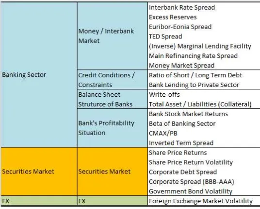
Figure 1:Variables included in the euro area financial sector data set
the annual growth rate of bank lending to the private sector, reflect dynamics of the theoretical models recently developed as response to the financial crisis (see, for instance, Brunnermeier and Sannikov, 2014 and Mittnik and Semmler, 2013). Their macro-finance models have shown a critical impact of the banking sector on the real economy, such that the balance sheet structure of banks, credit conditions or credit constraints should be prominently considered in a financial sector data set.
We collected 21 series for 11 countries representing financial market conditions
and vulnerabilities which are presented in Figure 1.5They can be classified in three
broad categories: variables for the banking sector, the securities market and the foreign exchange market.
The financial sector data set consists of several variables representing the bank-ing sector. It is categorised in four segments: the money and interbank market, credit conditions and constraints, the balance sheet structure of banks, and banks’ profitability situation. The variables choice is based on two research strands: stan-dard neoclassical and non-neoclassical transmission channels following Boivin et al. (2011). The former channel can be categorised in an investment-based, trade-based or consumptions-based channel. To put it in a nutshell, higher interest rates reduce investments, consumption or demand for assets, thereby lowering output. Inter-est rates are captured by various variables in our data set such as interbank rate spreads, TED spreads or money market spreads to mention a few. We also put a
5 In compiling our data set we were inspired by Blix Grimaldi (2010), Cardarelli et al. (2011), Holló
focus on the non-neoclassical channel when explaining and theorising financial market stress. Foremost, the non-neoclassical channel is associated to a credit view, namely, that frictions in the supply or demand of credit lead to financial sector distortions. Frictions can then translate into financially distressed economies. Specifically, credit conditions and the balance sheet structure of banks relate to the recent non-neoclassical channel introduced by Brunnermeier and Sannikov (2014)
and Mittnik and Semmler (2013).6
Variables related to the money and interbank market express the liquidity and confidence situation in the banking-sector. These give an impression about the lending across financial institutions. A low level of liquidity or evolving mistrust leads to a decrease of supply or demand in the money market, leading to an increase in the spread. To this category belong excess reserves, the (inverse) marginal lending facility, interbank rate spreads, Euribor-Eonia spreads, TED spreads, main refinancing rate spreads, and money market spreads. The latter five are often subsumed under the term credit spreads.
If the interbank market fails or if savers are not willing to hold their money at banks due to uncertainty, banks have to constrain their credit and lending. This is represented by variables related to credit conditions and constraints such as the ratio of short to long term debt securities issued or bank lending to the private sector. In times of high financial stress, banks might be reluctant to issue credit or to offer long-term financing instruments to secure their liquidity position. This leads to lower bank lending to the private sector (non-financial institutions and households) putting pressure on the financing situation of corporations, for instance. As a result, credit conditions worsen and the probability for a credit crunch increases.
The balance sheet structure of banks gains increasingly importance in the literature as a potential financial market stress channel (Brunnermeier and Sannikov, 2014 and Mittnik and Semmler, 2013). Asset price losses or a decline in credit quality lead to a reduction in the value of bank assets. Hence, banks cut back or sell assets (firesales) which is then reflected in the balance sheet structure of banks. A decrease in collateral, an important indicator for the provision of credit, may then result in a cut back of credit, putting the financial sector under pressure and thus, increasing the default risk of financial institutions as well as of the private sector. We attempt to capture the implications of this strand of literature by incorporating write-offs and the ratio of total assets divided by liabilities as a proxy for the bank’s leverage ratio in our data set.
6 Naturally, the variables do not reflect only one strand of the literature but can also be associated to
The bank’s profitability situations is reflected in bank stock market returns,
betas of the banking sector, CMAX/PB,7and the inverted term spread. The higher
bank profitability, the more lending takes place, supporting financial stability and economic growth and vice versa.
The financial conditions in the securities market are expressed by share price returns and their volatility, corporate debt spreads and volatility of government bond returns. These variable express uncertainty in securities market related to debt overhang of corporates; thus, capturing stress associated with the sovereign debt crisis that unfolded in 2011.
A volatility variable reflecting risk in the foreign exchange market is included as well. This indicator should capture the risk of a currency crisis.
Most of the variables are country-specific, but some refer to the euro area aggregate. From our perspective, it is not sufficient to focus only on aggregated euro area series. Such variables would not reflect the heterogeneity of the financial sector of the individual euro area member states adequately (see also Bijlsma and Zwart, 2013). Table 8 in the Appendix provides a detailed description of the data, including transformations and sources. The financial series are available for Belgium, Germany, Austria, Finland, France, Greece, Ireland, Italy, Netherlands, Portugal and Spain from January 2002 to December 2012 on a monthly basis constituting a balanced sample. The selected euro area countries account for almost 98% of total euro area GDP which can be seen as representative for the euro area.
2.2 Methodology
We employ a factor model to explore the correlation structure in our large data set and to extract common factors, but do not impose a priori a one-common-factor structure as it is state of the art. Instead, we will firstly determine the number of latent static and dynamic factors with the help of the procedures by Bai and Ng
(2002) in combination with theτ-method and Bai and Ng (2007). Robustness of
our results will be assessed by means of tests procedures by Ahn and Horenstein
(2013), Alessi et al. (2010), and Hallin and Liška (2007).8 In a second step, we plug
in the estimated number of factors in a multi-factor model and estimate them with the method proposed by Doz et al. (2011). Since we only estimate the vector space spanned by the static factors, they are not uniquely identified. In order to enable the interpretation of the estimated factors we apply a rotation that is based on a
7 According to Illing and Liu (2006) and Holló et al. (2012) the CMAX measures the maximum
cumulated loss over a moving window. In order to capture the market valuation it is multiplied by the inverse of the price-to-book (PB) ratio.
8 We refer the reader to Barhoumi et al. (2013) or Breitung and Pigorsch (2013) who give an overview
prediction criterion. Finally, we uncover the “economic meaning” of the rotated factors with the aid of regression techniques.
The dynamic factor model (DFM) that we use has been outlined rich enough in the literature (e.g. Stock and Watson, 2005) and we only briefly sketch the set-up in order to organise ideas and to provide an intuition for the testing and estimation strategy. The DFM is an appropriate tool to model and explore the strong co-movement of the many time series in our data set. It is able to distinguish between factors and underlying shocks and allows us to get more detailed insights into factors related to financial stress and conditions in the euro area. The DFM reads as follows
xit=λi′0ft+· · ·+λis′ft−s+eit (1)
wherexit is the observed financial variablei(i=1, . . . ,N) at timet(t=1. . .T) and
ft is aq-dimensional vector ofqcommon dynamic factors. The vectorsλi0, . . . ,λis
are eachq-dimensional and contain the correlation coefficients between the variables
and the dynamic factors and their lags (dynamic factor loadings).eit is a stationary
idiosyncratic component with some form of weak cross-correlation, i.e. the much larger part of the covariation in the data is due to the shared factors than driven by
the idiosyncratic component that is governed byNvariable-specific shocks.
For estimating the number of primitive shocks, Bai and Ng (2007) firstly extract
the static factors, whose numberrcan be consistently estimated with the criteria of
Bai and Ng (2002), by means of static principal components. Then, a VAR(p) is
fitted to the factor estimates and a selection rule, that is based on the eigenvalues
of the residual covariance matrix, is applied. The idea of the test is that ar×r
semipositive definite matrix of rankqhasqnonzero eigenvalues and that a sequence
of test statistics on the ordered eigenvalues of the VAR’s residual covariance matrix converges to zero if the considered rank is greater than the true one.
The system can be solved with the Kalman filter and smoother recursion. Doz et al. (2011) propose a two-step procedure to estimate the unknown parameters of the system and to consistently recover the latent factors when the number of static and dynamic factors is known. In a first step, preliminary estimates of the parameters and latent factors are computed with the aid of a static principal components analysis (PCA). In a second-step, these estimates are fed into the Kalman filter recursion and the factor estimates are computed with the Kalman smoother. By precisely specifying heteroskedasticity of the idiosyncratic component and the factor dynamics the Kalman smoother helps to achieve possible efficiency improvements over factor estimates from principal components.
However, the factors and loadings are not unique and identified only up to a rotation. In the following, we use a similar rotation technique that has been applied by Canova and de Nicolo (2003) and Eickmeier (2005).
Our aim is to summarise the information in the financial sector data that is at best connected to real economic activity and to obtain factors that send early warning signals for the spill-over of financial stress to the real economic sectors. Thus, we pick a rotation that minimises the residuals from the following one-step direct forecast regression equation
in whichyt denotes quarterly GDP growth and ˆft is the vector that contains the
first and second principal component of the static principal component analysis, transformed by taking quarterly averages to match the observation frequency of
GDP.9 We choose the first and second principal component as a predictor for
future GDP growth in addition to own lagged values. Both components together explain more than 50% of the variance in the data and therefore summarise the most important part of the co-movement in the financial sector data. The rotation search
is implemented with the aid of a Givens matrixP(θ).
3 Results
The main questions of the paper are whether the data should be used to summarise its information in one single indicator or whether it carries information that reveals a richer dimension of the factors and shocks that drive financial stress or financial conditions. We first present results of the tests on the number of static and dynamic factors before we proceed to estimate the factors and attempt to give them an economic interpretation.
3.1 The number of static and dynamic factors
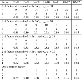
Table 1 shows the test results for the number of dynamic and static factors over sev-eral rolling sub-periods and the whole sample period. We firstly need to determine
9 In order to get an observationally equivalent model, we have to apply the rotation to the principal
component factors since these are orthogonal by construction. The Kalman smoother factor estimates are not exactly orthogonal due to smoothing so rotating the smoothed factors is not an option.min
equation (2) is set to zero so we consider the first two principal components without lags andpis set
Table 1:Estimated number of static and dynamic factors
Period 02-07 03-08 04-09 05-10 06-11 07-12 02-12
♯of factors determined withBIC3,rmax=30
Notes:rˆis the estimated number of static factors.BIC3denotes the information criterion
by Bai and Ng (2002). ˆqdenotes the estimated number of dynamic factors from the testing procedure by Bai and Ng (2007).τis the fraction of variation in the data that is explained by the common factors. The optimal lag length of the VAR in the static factors is determined with the Schwarz Information Criterion (SIC).
the number of static factors. This number has to be defined in order to test how many dynamic factors explain the variance of the data. To find the number of static
factors we apply the information criteriaICp1andBIC3of Bai and Ng (2002). Both
require to fix a maximum number of factors (rmax) that are to be tested in order to
determine the optimal number. There is no formal criterion to selectrmaxso we try
several values. TheICp1always selects a number of static factors that is equal to
rmax, the maximum number of tested factors, so we do not report these results.10
TheBIC3criterion reaches a minimum at ˆr=23 over the whole sample when
the maximum number of static factors is set to 30. These 23 factors together explain
10Empirical applications of the Bai and Ng (2002) criteria often report similar results. Forni et al.
(2009), for instance, conclude that theICp1criteria does not work in selecting ˆrapplied to a U.S.
0 2 4 6 8 10 12 14 16 18 20 0
0.05 0.1 0.15 0.2 0.25 0.3 0.35
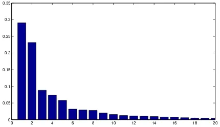
Figure 2:Explained fraction of the total variance by the principal components
96% of the total variance in the data. If we setrmaxequal to 10,BIC3selects 9 static
factor being optimal to explain the common variation in the data which together account for 85% of the variance. Since the information criterion does not give clear
guidance to the selection of ˆr, we additionally select the number of static factors by
setting a threshold value for the minimum fraction of variance that the factors need to
explain (τmethod).11If we select ˆrsuch that at least 80% of the variance in the data
is explained, we end up with 8 static factors for the whole sample period that explain
83% of common variation. Settingτ ≥0.6 results in 3 static factors estimated over
the whole sample range. A slightly higher number of ˆr, namely 5, would be selected
by the decision rule proposed by Forni et al. (2000) which adds factors until the additional variance explained by the last dynamic principal component is less than a pre-specified fraction, typically 5% or 10%, of total variance. Figure 2 shows this fraction for the ordered principal components. The first component individually explains 29%, the second 23%, the third 9%, the fourth 7% and the fifth 6%. Less than 5% of the total variance is individually explained from the sixth component on. The last rows of Table 1 display results if we select only one static factor which does not explain even half of the variation in the observables.
Table 1 also shows that the estimated number of primitive shocks ˆqis limited
and lies between 1 and 2 if we focus on the whole sample period from 2002 to
2012 and rule out the extreme selection by theBIC3whenrmax=30. Thus, a much
smaller number of dynamic factors than static ones suffices to explain the variation in the data. How can we relate the relatively large number of static factors to the more narrow fundamental sources of shocks? Forni et al. (2009) show that the more heterogeneous the dynamic responses of the common components to the primitive
shocks, the bigger isr with respect to q. Thus, our test results suggest that the
data respond quite differently to fundamental shocks to financial markets but the
11Bai and Ng (2007) also consult theτ criterion in their empirical application although it is not
dimension of these shocks is rather limited. Hence, countries or segments of the financial sector react fairly heterogeneously to such shocks. We clearly identify different factors in our financial sector data set which will be explored in the next section in more detail. As regards stability of the number of factors over time, Table 1 shows that the estimated numbers of static and dynamic factors vary more between
the approaches to fix ˆrthan between subperiods.
3.2 The factor estimates and rotation
We estimate our default model with eight static and two dynamic factors. The previous section has shown that it is difficult to obtain clear results with respect to the static factors but that the number of primitive shocks is always limited to lie between one and three. We want to specify a parsimonious factor model because we estimate the factors with the Kalman filter and smoother that does not work properly if we have a too rich state space model. From our view, eight static factors seem to be a good choice to account for the latter as well as the results of the statistical
criteriaBIC3andτ. Eight static factors explain more than 80% of the variation in
the data. Including another factor adds only 2% in explanatory power, but would most likely affect our estimations adversely.
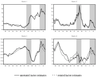
Figure 3 depicts the unrotated and rotated factor estimates obtained from the Kalman smoother. We only show the first four estimates since these together explain
almost 70% of the total variance of the data.12 The unrotated and the rotated factor
estimates are similar but the degree of “smoothness” and variability of the estimated
factors is quite diverse.13 The first factor estimate carries a common component
that signals a level shift between the period before and after the Lehman default (marked by a vertical line in September 2008), whereas the second factor estimate clearly depicts the temporary high stress in financial markets during the peak of the banking crisis and during the later period when extensive levels of public debt in the euro area sparked concerns about sovereign default and the future of the currency union. Furthermore, the marked jumps in Factor 1 and 2 coincide with the recession periods that have been classified by the European Business Cycle Committee. Factor 3 steadily increased during tranquil economic periods and dropped during times of
12Recall that we estimate our whole model with eight factors to work with a well-defined factor
model. Yet, we abstract from showing the four further factors as their explanatory power is negligible.
13A word on robustness of the rotation is appropriate at this point. We implemented the rotation with
-10
—
unrotated factor estimates· · ·
rotated factor estimatesMonths that belong to quarters which have been dated by the CEPR Business Cycle Dating Committee as periods of recessions are indicated in grey (see http://www.cepr.org/content/euro-area-business-cycle-dating-committee).
Figure 3:Factor estimates
recession. As we show below, this factor is strongly related to the yield curve and the profitability situation of European banks. The behavior of the fourth factor can be interpreted only with difficulty by eyeballing. We leave this open at this point, but will come back to the interpretation of the factor in the next section.
towards systemic financial stress. It captures stress periods where the whole financial system is under pressure, similar to the CISS indicator developed by Holló et al. (2012).
Robustness
We further explore the robustness of our result by considering further test procedures on the number of static and dynamic factors and by estimating the DFM of Doz
et al. (2011) with potential alternative values ofr andqin order to check if our
main results survive different model settings.
In a first step, we apply the eigenvalue ratio test by Ahn and Horenstein (2013)
to determine the number of static factorsrwhich results in a quite parsimonious
model by favouring two static factors. Given two static factors, the Bai and Ng (2007) test selects one dynamic factor. The fraction of explained variance amounts to slightly above 50%. The model seems to be a good compromise between the very high number of factors selected by the Bai and Ng (2002) criteria and the one factor model.
When we estimate the factors with the two-step procedure by Doz et al. (2011) and specify two static factors and one dynamic factor and compare the results, we do not find remarkable differences between the smoothed estimates of factor 1 and 2 of this model and our default model that specifies 8 static and 2 dynamic factors. In a further step, we explore the modified version of the Bai and Ng (2002) procedure by Alessi et al. (2010) to determine the number of static factors that improves the performance of the original test principle in empirical applications. The aim is to cure the well known problems of the Bai and Ng (2002) criteria in empirical implementations to deliver non-robust results regarding the estimated number of factors as they are often over or under-estimated (see Alessi et al., 2010). Results suggest 5 static factors. The Bai and Ng (2007) test in turn determines one dynamic factor from the 5 static ones. Estimating the DFM with these settings results in static factor estimates that are again very similar to the ones from our default model.
For a final robustness check, we determine the number of dynamic factors with
the procedure by Hallin and Liška (2007) which is valid for thegeneraldynamic
factor model (in contrast to therestricteddynamic model that applies for the Bai
From these additional analyses we conclude that our general results are quite robust and the smoothed factor estimates are insusceptible to minor alterations of central model parameters. To sum up, the test results clearly suggest that the true number of factors is greater than one and that more than only one primitive shock drive the individual indicators of financial stress. Furthermore, as the estimated number of primitive shocks is small compared to the estimated number of static factors, heterogeneity of responses of the financial variables to these shocks seems to be another salient feature of our data set.
3.3 Exploratory analysis
Next, we provide a more exploratory characterisation of the factor estimates. The
subsequent tables display the highestR2’s of the regressions of the financial sector
data against each of the first and second estimated rotated factors to assess for which individual financial indicator in which country the common factors have high explanatory power. In addition, we regress economic variables on each of these factors to explore whether the factors are linked to real economic activity and economic sentiment, measured by the annual growth rate of industrial production
and the Economic Sentiment Indicator from the European Commission.14
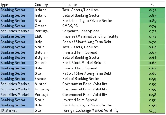
TheR2’s sorted in descending order that are displayed in Table 2 point to high
loadings of Factor 1 on variables that are related to the banking sector, particularly in those euro area periphery countries that have been hit most severe by the financial market crisis such as Ireland, Greece, Spain, Portugal, and Italy. Balance sheets of banks have deteriorated in almost all euro area countries since the outburst of the financial crises in 2008. This is clearly reflected in permanent decreases of the assets to liabilities ratios which indicates a reduction in collateral, increasing betas that echo riskier banking sectors and a deteriorating bank lending to the private sector. Factor 1 is characterised by variables that specifically reflect adverse credit conditions and constraints in the periphery countries of the euro area. They point towards an increasing probability for a credit crunch. In times of high financial market uncertainty, banks might be reluctant to issue credit to secure their liquidity position. Default risk of financial institutions and of the private sector reflected in
the variables that load high on Factor 1 are crucial, shown by highR2s of the assets
over labilities as proxy for bank’s leverage ratio. The estimated Factor 1 loads on these and other aspects that are related to the euro area banking crisis and hence may be labeled a “Periphery Banking Crisis” factor. The factor estimate shows a
14Note that we check the correlation of financial sector and economic data and the factor estimates.
Table 2:R2between rotated Factor 1 and the financial sector variables
Type Country Indicator R2
Banking Sector Ireland Total Assets/Liabilites 0.91 Banking Sector Ireland Beta of Banking Sector 0.87 Banking Sector Spain Bank Lending to Private Sector 0.83 Banking Sector Greece CMAX/PB 0.74 Securities Market Portugal Corporate Debt Spread 0.73 Banking Sector EMU (Inverse) Marginal Lending Facility 0.71 Banking Sector Italy Ratio of Short/Long Term Debt 0.70 Banking Sector Spain Total Assets/Liabilites 0.69 Banking Sector Belgium Inverted Term Spread 0.67 Banking Sector Belgium Beta of Banking Sector 0.66 Banking Sector Greece Bank Stock Market Returns 0.64 Banking Sector Italy Inverted Term Spread 0.61 Banking Sector Spain Ratio of Short/Long Term Debt 0.60 Banking Sector France Beta of Banking Sector 0.59 Securities Market Austria Government Bond Volatility 0.59 Securities Market Germany Government Bond Volatility 0.59 Securities Market Portugal Government Bond Volatility 0.58 Banking Sector Spain Inverted Term Spread 0.58 Banking Sector Italy Bank Lending to Private Sector 0.56 FX Market Spain Foreign Exchange Market Volatility 0.55
Note:The left column describes the type of indicator: banking sector (deep blue), securities market (blue), foreign exchange (fx) market (light blue). The right column presents the results ofR2in descending order, thereby showing in green colour the size ofR2(the darker the green is, the higher is theR2).
level shift which further confirms our interpretation as the banking sector is still not free from pressure in periphery countries. This supports persisting fragilities in the banking sector which were reinforced by the sovereign debt crisis setting in quite heavily in 2011.
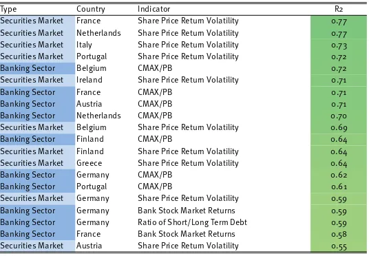
Table 3:R2between rotated Factor 2 and the financial sector variables
Type Country Indicator R2
Securities Market France Share Price Return Volatility 0.77 Securities Market Netherlands Share Price Return Volatility 0.77 Securities Market Italy Share Price Return Volatility 0.73 Securities Market Portugal Share Price Return Volatility 0.72 Banking Sector Belgium CMAX/PB 0.72 Securities Market Ireland Share Price Return Volatility 0.71 Banking Sector France CMAX/PB 0.71 Banking Sector Austria CMAX/PB 0.71 Banking Sector Netherlands CMAX/PB 0.70 Securities Market Belgium Share Price Return Volatility 0.69 Banking Sector Finland CMAX/PB 0.64 Securities Market Finland Share Price Return Volatility 0.64 Securities Market Greece Share Price Return Volatility 0.64 Banking Sector Germany CMAX/PB 0.62 Banking Sector Portugal CMAX/PB 0.61 Securities Market Germany Share Price Return Volatility 0.59 Banking Sector Germany Bank Stock Market Returns 0.59 Banking Sector Germany Ratio of Short/Long Term Debt 0.59 Banking Sector France Bank Stock Market Returns 0.58 Securities Market Austria Share Price Return Volatility 0.55
Note:The left column describes the type of indicator: banking sector (deep blue), securities market (blue), foreign exchange (fx) market (light blue). The right column presents the results ofR2in descending order, thereby showing in green colour the size ofR2(the darker the green is, the higher is theR2).
For the design of an effective economic policy which may be warranted if a high level of financial stress is imminent the source of financial stress is of utmost importance. Factor 1 and Factor 2 reveal different sources of financial stress in the euro area. Factor 1 indicates that stress originates from a group of (periphery) countries. This happened in the Eurozone several times since 2008 because its periphery member states nearly defaulted. In such a scenario, country-specific and immediate responses in the form of sovereign and private aid programmes matter and may be the road to success. During times in which stress is triggered by the banking sector as indicated by Factor 2, however, monetary policy and micro-macro prudential policies may be more powerful. These two examples highlight that insights into the sources of financial stress are important for selecting and preparing the appropriate policy response.
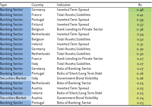
Factor estimate 3 again is most closely connected to variables from the banking sector, in particular those that are related to bank’s profitability situation (inverted term spread) and bank’s balance sheet structure (as measured by total assets over liabilities). See Table 4. The results are more mixed across countries, but with
the highestR2’s in the regressions with data form the Nordic and core euro area
countries. Due to its mimicking of the yield curve slope we denote this factor
estimate a “Yield Curve” factor. The regression’sR2’s for the fourth factor estimate
Table 4:R2between rotated Factor 3 and the financial sector variables
Type Country Indicator R2
Banking Sector Germany Inverted Term Spread 0.48 Banking Sector France Total Assets/Liabilites 0.41 Banking Sector Portugal Inverted Term Spread 0.39 Banking Sector Finland Inverted Term Spread 0.37 Banking Sector Belgium Bank Lending to Private Sector 0.36 Banking Sector Netherlands Inverted Term Spread 0.34 Banking Sector Belgium Total Assets/Liabilites 0.32 Banking Sector Ireland Inverted Term Spread 0.31 Banking Sector Germany Total Assets/Liabilites 0.30 Banking Sector Netherlands Total Assets/Liabilites 0.30 Banking Sector France Bank Lending to Private Sector 0.27 Banking Sector Italy Total Assets/Liabilites 0.27 Banking Sector Germany Beta of Banking Sector 0.27 Banking Sector Portugal Ratio of Short/Long Term Debt 0.26 Securities Market Italy Government Bond Volatility 0.26 Banking Sector Netherlands Beta of Banking Sector 0.25 Banking Sector Austria Inverted Term Spread 0.25 Banking Sector Ireland Ratio of Short/Long Term Debt 0.25 Securities Market Austria Government Bond Volatility 0.24 Banking Sector Portugal Beta of Banking Sector 0.23
Note:The left column describes the type of indicator: banking sector (deep blue), securities market (blue), foreign exchange (fx) market (light blue). The right column presents the results ofR2in descending order, thereby showing in green colour the size ofR2(the darker the green is, the higher is theR2).
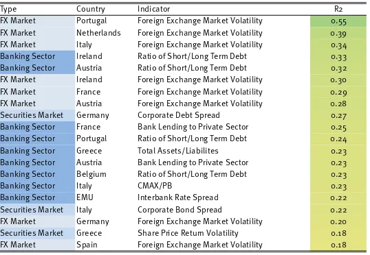
interpretation as a “Foreign Exchange Rate Volatility” factor that is in particular relevant for Portugal, Italy and the Netherlands.
The regressions of the financial sector data on the remaining four factors reveal only marginal explanatory power so we skip an exposition. More illuminating are the relations between the factor estimates and data for the real economy. Such supplementary variables are used to enrich the interpretation of the factors. Re-gressions of the Economic Sentiment Indicators of the European Commission and annual growth rates of industrial production on the first four factor estimates reveal
interesting results.15 Factor 1 is related to economic sentiment, which has been
deteriorating in particular in Greece, Portugal, Spain, Italy and Ireland since 2008. These results underline that Factor 1 is related to the crises in the periphery countries which are closely connected to the unhealthy situation in the banking sector. The
R2’s in the regressions that contain industrial production are low and imply that
Factor 1 is more related to sentiment than to real economic activity. However, the explanatory power of Factor 2—the “Stress” factor—is generally higher for the annual growth rate of industrial production than for economic sentiment. This is in line with the recent literature strand linking financial stress to the real economy. Amongst others, Hubrich and Tetlow (2013), Mittnik and Semmler (2013), Holló
Table 5:R2between rotated Factor 4 and the financial sector variables
Type Country Indicator R2
FX Market Portugal Foreign Exchange Market Volatility 0.55 FX Market Netherlands Foreign Exchange Market Volatility 0.39 FX Market Italy Foreign Exchange Market Volatility 0.34 Banking Sector Ireland Ratio of Short/Long Term Debt 0.33 Banking Sector Austria Ratio of Short/Long Term Debt 0.32 FX Market Ireland Foreign Exchange Market Volatility 0.30 FX Market France Foreign Exchange Market Volatility 0.29 FX Market Austria Foreign Exchange Market Volatility 0.28 Securities Market Germany Corporate Debt Spread 0.27 Banking Sector France Bank Lending to Private Sector 0.25 Banking Sector Portugal Ratio of Short/Long Term Debt 0.24 Banking Sector Greece Total Assets/Liabilites 0.23 Banking Sector Austria Bank Lending to Private Sector 0.23 Banking Sector Belgium Ratio of Short/Long Term Debt 0.23 Banking Sector Italy CMAX/PB 0.23 Banking Sector EMU Interbank Rate Spread 0.22 Securities Market Italy Corporate Bond Spread 0.22 FX Market Germany Foreign Exchange Market Volatility 0.20 Securities Market Greece Share Price Return Volatility 0.18 FX Market Spain Foreign Exchange Market Volatility 0.18
Note:The left column describes the type of indicator: banking sector (deep blue), securities market (blue), foreign exchange (fx) market (light blue). The right column presents the results ofR2in descending order, thereby showing in green colour the size ofR2(the darker the green is, the higher is theR2).
et al. (2012) and Schleer and Semmler (2013), find a persistent, negative response of economic activity after a shock in the financial sector which is more severe if this shock took place in a high financial stress regime.
The third factor which is connected to the yield curve and the profit situation of the banking sector loads higher on the sentiment indicators of the Nordic and core euro area countries such as Germany and the Netherlands than on the economic
data for the Southern countries. TheR2’s of the regressions from the fourth factor
are low and do not warrant meaningful interpretations. Taken together, these further results imply that the estimates of the first three factors share information with observations for economic sentiment and real economic activity and confirm our initial interpretation of these factors.
3.4 Out-of-sample forecasting exercise
To evaluate the forecasting ability of our factor estimates, we perform a pseudo out-of-sample forecasting evaluation for euro area economic activity that simulates
realtime forecasting.16 Having found that several common factors optimally explain
16We do not control for publication lags, i.e. the forecast for 2008m01 is based on the first release
the in-sample co-movement of the financial sector data set, we now ask whether one or more of the estimated factors also improve forecast accuracy for industrial production growth in the euro area. In order to evaluate the out-of-sample accuracy, we build several VAR-models using real-time monthly log growth rates of the euro
area industrial production and real-time estimated factor(s).17 IP vintages provided
by the OECD are used for the real-time exercise. In section 3, we show that the number of factors rather varies across testing procedure than across time. Thus, we estimate eight real-time factors—identified by the procedures in Section 3 and used in our default model—for each forecast model.
Model VAR_1 consists of monthly IP growth and the first factor (“Periph-ery Banking Crisis”), model VAR_2 of monthly IP growth and the second factor (“Stress”), and so on. Additionally, we estimate a VAR model with the first and the second factor (VAR_12, responsible for 50% of the variation in the data), similarly VAR_123 and VAR_1234 are augmented by the respective factor and finally, a VAR model that comprises all eight factor suggested by our default model (VAR_1-8).
To evaluate the forecast accuracy of the individual forecast models, we calculate the root mean squared forecast error (RMSFE) for each model and the respective forecast horizon. The first sample period covers the months from 2002m01 to 2007m12 and is then gradually augmented to evaluate the subsequent monthly forecast horizons. The RMSFE is calculated over all forecast errors up to the final
forecast horizon (Th) as indicated by the following formula:
RMSFEh=
in whichThdenotes the number of forecasts,hthe forecast horizon,xt+his the
actual value of industrial production in real-time and ˆx(t+h),t is theh-month ahead
forecast produced at timet. Multi-step forecasts rely on iterating the VAR forward.
We use the third releases of the OECD vintage data to compute forecast errors to avoid strong revisions in the first months. However, our results are robust for the first and second official release of industrial production data.
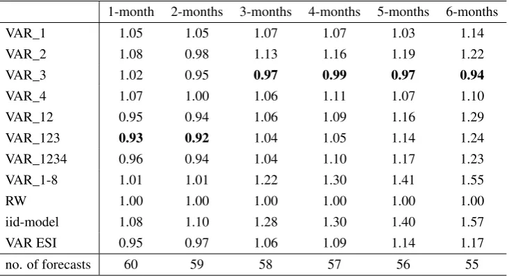
As benchmarks we use a standard random walk forecast based on random walk without drift (RW), a forecast that is based on an iid-model such that the forecast defines the recent sample mean, and a bivariate VAR using industrial production and the economic sentiment indicator (VAR ESI) for the euro area. The RMSFE’s for one to six month ahead forecasts of the VAR models relative to the random walk model are shown in Table 6. We have chosen the random walk as a benchmark since the iid model always performs worse than the random walk.
17We decide to use VAR models instead of a univariate model to capture interdependent effects
Table 6:Root mean squared forecast error relative to the random walk model (RW), 1–6 months forecast horizon
1-month 2-months 3-months 4-months 5-months 6-months
VAR_1 1.05 1.05 1.07 1.07 1.03 1.14
VAR_2 1.08 0.98 1.13 1.16 1.19 1.22
VAR_3 1.02 0.95 0.97 0.99 0.97 0.94
VAR_4 1.07 1.00 1.06 1.11 1.07 1.10
VAR_12 0.95 0.94 1.06 1.09 1.16 1.29
VAR_123 0.93 0.92 1.04 1.05 1.14 1.24
VAR_1234 0.96 0.94 1.04 1.10 1.17 1.23
VAR_1-8 1.01 1.01 1.22 1.30 1.41 1.55
RW 1.00 1.00 1.00 1.00 1.00 1.00
iid-model 1.08 1.10 1.28 1.30 1.40 1.57
VAR ESI 0.95 0.97 1.06 1.09 1.14 1.17
no. of forecasts 60 59 58 57 56 55
Notes:Bold number indicate the best forecasting model and thereby, also the minimum over the forecast horizon relative to the random walk model.
VAR_1 consists of monthly IP growth and the first factor (“Periphery Banking Crisis”), model VAR_2 of monthly IP growth and the second factor (“Stress”), and so on. RW is a standard random walk model without drift, iid-model defines the (recent) sample mean, and VAR ESI is a bivariate VAR using industrial production and the economic sentiment indicator.
Interestingly, for short forecast horizons a VAR model containing the first three factors—the “Periphery Banking Crisis”, the “Stress”, and the “Yield Curve” factor—performs best indicating that extracting only a single stress factor may not always yield the best forecast for economic activity. Thus, for the short-term forecast horizon, it seems to be beneficial to take several risk dimensions into account. Interestingly, the metrics in Table 6 suggest that there is a switch in forecasts performance between 2-months (multi-factor model) and 3-months (one-factor model) forecasting horizons. A model containing only the “Yield Curve” factor (third factor), however, yields lower RMSEs relative to the RW model for horizons that are longer than two months. Hence, the term transformation—an indicator for the profitability of banks—gains importance. To put it differently, the third factor seems to incorporate economically relevant information of the financial sector that dominate the other factors, the “Periphery Banking Crisis” and “Stress” factor that jointly yield predictive information at short terms in the euro area.
find that the one-factor model performs at least as well as the more factor variant when looking at a 2- and 4-months forecast horizon.
While some VAR models containing only one factor are beaten by the “recent mean” forecast, this does not hold for most models with more factors. Additionally, the best-performing factor VAR model does also produce better forecasts than a bivariate VAR using the economic sentiment indicator.
Some qualitative results hold if we augment all “factor”-VAR models (VAR_1 –
VAR_1-8) by the Economic Sentiment Indicator (ESI).18For the two-month horizon,
a VAR with more than one factor (VAR_12) has a higher forecast accuracy than the VAR using only euro area economic activity and the ESI for the two-month horizon. At longer horizon, the forecasts even worsen compared to “factor”-VAR models without economic sentiment shown in the previous table. The one-factor model, however, is better than multi-factor models at the 1-month horizon.
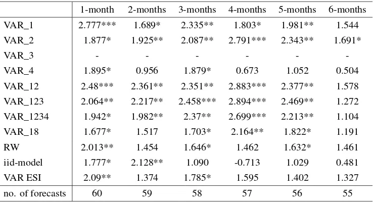
As regards significance with respect to forecast accuracy, we run tests of equal mean squared prediction errors (MSPE) in nested models as suggested by Clark and West (2007). The tests allow only bilateral comparison so we benchmark VAR_3, which produced the forecasts with the lowest root mean squared error for longer horizons, vis-Ã -vis the other models. The null hypothesis of the Clark and West (2007) test is that two forecasts have the same MSPE. We find that VAR_3 (which contains only the yield-curve factor) generates statistically significantly better forecasts than most other models for horizon 1 to 5, but the statistics are insignificant for a forecast horizon of 6 months (see Table 7). Thus, we cannot rule out that the performance dominance of the “Yield Curve” factor model as suggested by the metrics in Table 6 is due to sampling error. The sample size is quite small, therefore the statistics may be fragile and results not very generalizable.
Taken together, the results lend some support to our previous analysis that a single indicator might not always be sufficient to gauge stress and risks that emerge from the financial sector and that may also be predictive for activity in the real sector at short horizons. In this subsection we have shown that including financial sector dimensions may to some extent improves the real-time forecasts of economic activity.
This result is very much in line with recent papers that demonstrate that financial indicators are useful for forecasting output growth in the euro area (Camacho and Garcia-Serrador, 2014). While forecaster typically augment their models with single financial indicators such as the yield curve or credit growth, we conjecture that it might even be worthwhile considering a broader set of financial sector information for forecasting purposes.
Table 7:Clark and West (2007) statistics, benchmark model is VAR_3
1-month 2-months 3-months 4-months 5-months 6-months
VAR_1 2.777*** 1.689* 2.335** 1.803* 1.981** 1.544
VAR_2 1.877* 1.925** 2.087** 2.791*** 2.343** 1.691*
VAR_3 - - -
-VAR_4 1.895* 0.956 1.879* 0.673 1.052 0.504
VAR_12 2.48*** 2.361** 2.351** 2.883*** 2.377** 1.578
VAR_123 2.064** 2.217** 2.458*** 2.894*** 2.469** 1.272
VAR_1234 1.942* 1.982** 2.37** 2.699*** 2.213** 1.104
VAR_18 1.677* 1.517 1.703* 2.164** 1.822* 1.191
RW 2.013** 1.454 1.646* 1.462 1.632* 1.461
iid-model 1.777* 2.128** 1.090 -0.713 1.029 0.481
VAR ESI 2.09** 1.374 1.785* 1.595 1.402 1.327
no. of forecasts 60 59 58 57 56 55
Notes:The null hypothesis is equal mean squared prediction error (MSPE). The alternative is that VAR_3 has a smaller MSPE than the alternative model. ***, **, * denote significance at the 1%, 5% and 10% level
4 Conclusion
In this paper we evaluate the co-movement of financial sector data from a newly compiled data set on stress and conditions in euro area financial markets. The data set extends existing compilations by variables related to the banking sector that have often been neglected, but proven to be crucial to understand the spillover of stress from the financial system to real economic activity. A lesson learned from the recent financial crisis is that closely monitoring banking-related factors should contribute to the improvement of tracking periods of financial distress.
test with the procedures by Bai and Ng (2002) combined with theτ-method and Bai and Ng (2007).
We find that the optimal number of static factors that explain the common movement lies between 8 and 9, but that the number of dynamic factors (the “primitive” shocks) is limited and lies between 1 and 2 if we focus on the whole sample period from 2002 to 2012. Thus, a much smaller number of dynamic factors than static ones suffices to explain the variation in the data. These results suggest that the individual time series respond quite differently to fundamental shocks to financial markets but the dimension of these shocks is rather limited. Robustness of the factor estimates is confirmed by using novel test procedures provided by Ahn and Horenstein (2013), Alessi et al. (2010), and Hallin and Liška (2007).
In a further step we attempt to give the estimated static factors an economic interpretation with the aid of an exploratory analysis. For that purpose, we regress the financial sector data against each of the first four estimated rotated factors and search for common patterns in the explanatory power of the factors. We concentrate on the first four factors since these together explain almost 70% of the total variance of the data and the further factors add only marginal explanatory power. From the exploratory analysis we conclude that the presence of a “Periphery Banking Crisis” factor, a “Stress” factor and a “Yield Curve” factor explains the bulk of variation in recent euro area financial sector data. Thus, financial conditions and stress in the euro area covers several dimensions that are insufficiently summarized by just one single indicator.
For the design of an effective economic policy which may be warranted if a high level of financial stress is imminent the source of financial stress is of utmost importance. The factors reveal different sources of financial stress in the euro area. Thus, understanding the impact of these factors is important for selecting and preparing the appropriate policy response.
The analyses of economic variables support the interpretation of our factor estimates. Economic sentiment in the southern euro area countries is closely related to factor one which coincides with our interpretation as a “Periphery Banking Crisis”. The second factor estimate, the “Stress” factor, is closely connected to industrial production which is in line with the recent literature linking financial stress to real economic activity.
Appendix
4.1 The Data
Economics:
Indicators Description Tcode N. Freq. Source First obs. Notes
BANKINGSECTOR
Interbank Rate Spread Interbank Offered Rate 12 m. - Interbank Offered Rate 1 m. 0 daily D country-spec. EA agg. Excess Reserves Bank reserves in excess of the central banks’ reserve requirement 1 monthly ECB 2000M01 EA agg. Euribor-Eonia Spread Interbank Offered Rate 1 m. - Eonia (effective overnight rate, unsecured lending) 0 daily D country-spec. EA agg. TED Spread Interbank Offered Rate 3m. - government short term rate 0 daily D country-spec. (Inverse) Marginal Lending Facility To obtain overnight liquidity from ECB 2 daily D (ECB) 1999M01 EA agg. Main Refinancing Rate Spread Euro area 2-y. benchmark bond yield - minimum bid rate 0 daily / monthly D 1999M01 EA agg.
Money Market Spread Euribor 3m. - EUREPO 0 daily D (ECB) 1999M05 EA agg.
Ratio of Short / Long Term Debt Debtsecuritiesissued<1year(short−term)and1−2years(medium−term)
dividedby>2years(long−term)o f MFIs 0 monthly ECB country-spec.
Bank Lending to Private Sector Bank lending to private sector in constant prices 3 monthly D country-spec. Write-offs MFIs, Loans to Nonfinancial Corporations and Households, Write-offs/write-down 1 monthly D 2002M01 EA agg. Total Assets / Liabilities MFIs Total Assets/Liabilities; Index of Notional Stocks 3 monthly ECB country-spec.
Bank Stock Market Returns Bank stock market returns 3 daily D country-spec.
Beta of Banking Sector Measure of banking risk relative to market risk 4 daily D country-spec. CMAX/PB Financial intermediary risk interacted with stock market valuation 5 daily D country-spec. Inverted Term Spread Slope of yield curve: short term government yield - long term government yield 0 monthly D country-spec. SECURITIESMARKET
Share Price Returns Stock markets returns 6 monthly D country-spec.
Share Price Return Volatility Stock markets volatility 7 monthly D country-spec.
Corporate Debt Spread AAA country specific corporate bond yield- Euro Area AAA corporate bond yield 0 monthly D country-spec. Corporate Spread (BBB-AAA) BBB Euro Area corporate bonds- AAA Euro Area corporate bonds 0 monthly D 1999M04 EA agg. Government Bond Volatility Volatility of long-term government bonds 7 monthly D country-spec. FOREIGNEXCHANGEMARKET
Foreign Exchange Market Volatility Effective exchange rates, narrow index (27 economies), real cpi 7 monthly D (BIS) country-spec.
0 - levels, no transformation
1 - annual log differences / annual growth rate 2 - multiplicative inverse
3 - annual log differences multiplied by−1
4 -β=covvar((r,mm)); r and m are total returns, at annual rates, of the banking sector index and the overall market index. Beta is calculated by using a one-year rolling time-frame. The banking beta was recorded only when it was greater than one, else it is set to 1.
5 - (1-current value of stock market index/maximum value over last 12 months) multiplied by book-to-price ratio 6 - monthly absolute differences multiplied by−1
7 - 6-months backward-looking rolling window, standard deviation
General Remarks - Greece: We do not include the inverted term spread due to its paradoxical evolution during the current financial and economic crisis and the CMAX is not multiplied by Price-to-Book ratio which has some extreme outliers at the beginning of 2011. Ireland: Due to unavailability the corporate bond spread cannot be included.
nal.org
4.2 Additional Tables
Table 9:R2between rotated Factor 1 and the economic variables
Type Country Indicator R2
Sentiment Greece Economic Sentiment Indicator 0.88
Sentiment Portugal Economic Sentiment Indicator 0.65
Sentiment Spain Economic Sentiment Indicator 0.54
Sentiment Italy Economic Sentiment Indicator 0.49
Sentiment Ireland Economic Sentiment Indicator 0.43
Industry Greece Industrial Production 0.43
Sentiment France Economic Sentiment Indicator 0.30
Industry Spain Industrial Production 0.27
Sentiment Netherlands Economic Sentiment Indicator 0.24
Sentiment Austria Economic Sentiment Indicator 0.21
Sentiment Finland Economic Sentiment Indicator 0.20
Sentiment Belgium Economic Sentiment Indicator 0.17
Industry Belgium Industrial Production 0.14
Industry Finland Industrial Production 0.13
Industry Italy Industrial Production 0.11
Industry Portugal Industrial Production 0.09
Industry Austria Industrial Production 0.08
Industry Netherlands Industrial Production 0.07
Industry France Industrial Production 0.05
Industry Ireland Industrial Production 0.04
Industry Germany Industrial Production 0.04
Sentiment Germany Economic Sentiment Indicator 0.01
Table 10:R2between rotated Factor 2 and the economic variables
Type Country Indicator R2
Industry Spain Industrial Production 0.33
Industry France Industrial Production 0.26
Sentiment Finland Economic Sentiment Indicator 0.23
Sentiment Spain Economic Sentiment Indicator 0.23
Sentiment Ireland Economic Sentiment Indicator 0.22
Industry Italy Industrial Production 0.20
Industry Germany Industrial Production 0.19
Industry Austria Industrial Production 0.18
Sentiment Belgium Economic Sentiment Indicator 0.17
Sentiment Austria Economic Sentiment Indicator 0.17
Sentiment France Economic Sentiment Indicator 0.17
Sentiment Germany Economic Sentiment Indicator 0.15
Industry Belgium Industrial Production 0.12
Sentiment Italy Economic Sentiment Indicator 0.11
Industry Portugal Industrial Production 0.11
Industry Finland Industrial Production 0.08
Industry Netherlands Industrial Production 0.06
Sentiment Netherlands Economic Sentiment Indicator 0.05
Industry Greece Industrial Production 0.03
Industry Ireland Industrial Production 0.02
Sentiment Portugal Economic Sentiment Indicator 0.02
Sentiment Greece Economic Sentiment Indicator 0.00
Table 11:R2between rotated Factor 3 and the economic variables
Type Country Indicator R2
Sentiment Germany Economic Sentiment Indicator 0.30
Sentiment Netherlands Economic Sentiment Indicator 0.23
Sentiment Austria Economic Sentiment Indicator 0.22
Industry Austria Industrial Production 0.22
Industry Finland Industrial Production 0.20
Sentiment Belgium Economic Sentiment Indicator 0.17
Industry Germany Industrial Production 0.17
Sentiment France Economic Sentiment Indicator 0.16
Sentiment Finland Economic Sentiment Indicator 0.14
Industry France Industrial Production 0.12
Industry Italy Industrial Production 0.08
Industry Spain Industrial Production 0.07
Industry Greece Industrial Production 0.06
Sentiment Ireland Economic Sentiment Indicator 0.05
Industry Belgium Industrial Production 0.04
Sentiment Spain Economic Sentiment Indicator 0.03
Industry Netherlands Industrial Production 0.02
Sentiment Greece Economic Sentiment Indicator 0.02
Industry Portugal Industrial Production 0.01
Sentiment Italy Economic Sentiment Indicator 0.01
Industry Ireland Industrial Production 0.00
Sentiment Portugal Economic Sentiment Indicator 0.00
Table 12:R2between rotated Factor 4 and the economic variables
Type Country Indicator R2
Sentiment Spain Economic Sentiment Indicator 0.10
Sentiment Netherlands Economic Sentiment Indicator 0.09
Sentiment Germany Economic Sentiment Indicator 0.08
Sentiment Belgium Economic Sentiment Indicator 0.05
Sentiment Portugal Economic Sentiment Indicator 0.04
Industry Greece Industrial Production 0.04
Sentiment Finland Economic Sentiment Indicator 0.03
Industry Spain Industrial Production 0.03
Industry Ireland Industrial Production 0.02
Sentiment Austria Economic Sentiment Indicator 0.02
Industry Belgium Industrial Production 0.01
Sentiment France Economic Sentiment Indicator 0.01
Sentiment Italy Economic Sentiment Indicator 0.01
Sentiment Greece Economic Sentiment Indicator 0.01
Industry France Industrial Production 0.01
Industry Netherlands Industrial Production 0.00
Industry Portugal Industrial Production 0.00
Industry Austria Industrial Production 0.00
Industry Germany Industrial Production 0.00
Industry Italy Industrial Production 0.00
Sentiment Ireland Economic Sentiment Indicator 0.00
Industry Finland Industrial Production 0.00
Table 13:Root mean squared error, 1–6 months forecast horizon, models augmented by economic sentiment
1-month 2-months 3-months 4-months 5-months 6-months
VAR_1 1.04% 1.14% 1.23% 1.33% 1.38% 1.49%
VAR_2 1.28% 1.28% 1.47% 1.51% 1.62% 1.67%
VAR_3 1.20% 1.22% 1.35% 1.41% 1.54% 1.49%
VAR_4 1.15% 1.21% 1.36% 1.48% 1.58% 1.61%
VAR_12 1.09% 1.11% 1.27% 1.30% 1.43% 1.55%
VAR_123 1.12% 1.12% 1.27% 1.33% 1.46% 1.57%
VAR_1234 1.14% 1.14% 1.29% 1.37% 1.50% 1.61%
VAR_1-8 1.18% 1.21% 1.48% 1.61% 1.79% 1.94%
recent mean 1.19% 1.20% 1.22% 1.23% 1.24% 1.23%
no change 1.28% 1.32% 1.57% 1.60% 1.74% 1.93%
VAR ESI 1.13% 1.17% 1.29% 1.35% 1.42% 1.44%
References
Ahn, S. C., and Horenstein, A. R. (2013). Eigenvalue Ratio Test for the Number of
Factors.Econometrica, 81(3): 1203–1227. URLhttp://onlinelibrary.wiley.com/
doi/10.3982/ECTA8968/abstract.
Alessi, L., Barigozzi, M., and Capasso, M. (2010). Improved Penalization for
Determining the Number of Factors in Approximate Factor Models. Statistics &
Probability Letters, 80(23-24): 1806–1813. URLhttp://www.sciencedirect.com/
science/article/pii/S0167715210002282.
Angelopoulou, E., Balfoussia, H., and Gibson, H. D. (2014). Building a financial conditions index for the euro area and selected euro area countries: What does
it tell us about the crisis? Economic Modelling, 38(C): 392–403. URL http:
//www.sciencedirect.com/science/article/pii/S0264999314000169.
Bai, J., and Ng, S. (2002). Determining the Number of Factors in Approximate
Factor Models.Econometrica, 70(1): 191–221. URLhttp://onlinelibrary.wiley.
com/doi/10.1111/1468-0262.00273/abstract.
Bai, J., and Ng, S. (2007). Determining the Number of Primitive Shocks in Factor
Models. Journal of Business & Economic Statistics, 25(1): 52–60. URLhttp:
//amstat.tandfonline.com/doi/abs/10.1198/073500106000000413.
Barhoumi, K., Darné, O., and Ferrara, L. (2013). Testing the
Num-ber of Factors: An Empirical Assessment for a Forecasting
Pur-pose. Oxford Bulletin of Economics and Statistics, 75(1): 64–
79. URL http://onlinelibrary.wiley.com/doi/10.1111/obes.12010/abstract?
userIsAuthenticated=false&deniedAccessCustomisedMessage=.
Bernanke, B. S., Gertler, M., and Gilchrist, S. (1999). The Financial Accelerator in a Quantitative Business Cycle Framework. In J. B. Taylor, and M. Woodford (Eds.),
Handbook of Macroeconomics, volume 1 of Handbook of Macroeconomics,
chapter 21, pages 1341–1393. Elsevier. URL http://www.sciencedirect.com/
science/article/pii/S157400489910034X.
Bijlsma, M. J., and Zwart, G. T. (2013). The Changing Landscape of Financial Markets in Europe, the United States and Japan. Working paper, BRUEGEL
Working Paper 2013/02. URLhttp://www.econstor.eu/handle/10419/78013.
Blix Grimaldi, M. (2010). Detecting and Interpreting Financial Stress in the Euro
Area. Working Paper Series No. 1214, European Central Bank. URL https: