Wigner Quantization of Hamiltonians
Describing Harmonic Oscillators Coupled
by a General Interaction Matrix
Gilles REGNIERS and Joris VAN DER JEUGT
Department of Applied Mathematics and Computer Science, Ghent University, Krijgslaan 281-S9, B-9000 Gent, Belgium
E-mail: [email protected], [email protected]
Received September 22, 2009, in final form November 20, 2009; Published online November 24, 2009
doi:10.3842/SIGMA.2009.106
Abstract. In a system of coupled harmonic oscillators, the interaction can be represented by a real, symmetric and positive definite interaction matrix. The quantization of a Hamil-tonian describing such a system has been done in the canonical case. In this paper, we take a more general approach and look at the system as a Wigner quantum system. Hereby, one does not assume the canonical commutation relations, but instead one just requires the compatibility between the Hamilton and Heisenberg equations. Solutions of this problem are related to the Lie superalgebras gl(1|n) andosp(1|2n). We determine the spectrum of the considered Hamiltonian in specific representations of these Lie superalgebras and discuss the results in detail. We also make the connection with the well-known canonical case.
Key words: Wigner quantization; solvable Hamiltonians; Lie superalgebra representations
2000 Mathematics Subject Classification: 17B60; 17B80; 81R05; 81R12
1
Introduction
In quantum as well as in classical mechanics, the harmonic oscillator is one of the most popular examples to describe harmonic movement of a particle. Their numerous applications and their analytical solvability as quantum systems explain why harmonic oscillator models are thoroughly investigated. Systems of interacting harmonic oscillators are among these well-known models. A system ofnone-dimensional harmonic oscillators interacting with each other can be described in its most general form as [1]
ˆ
H = ˆr†Vr.ˆ
In this equation, ˆr†is the vector (ˆp†
1, . . . ,pˆ†n,qˆ1†, . . . ,qˆ†n), with ˆqrand ˆpr respectively the position
and momentum operator of the oscillator at location r, and V is a positive definite matrix describing the coupling in position and momentum coordinates. In the present paper, we will assume that there is no coupling involving the momentum operators. Following this approach, we can write the Hamiltonian in the following manner:
ˆ H = 1
2m pˆ
†
1 · · · pˆ†n
ˆ p1
.. . ˆ pn
+
m 2 qˆ
†
1 · · · qˆn†
A
ˆ q1
.. . ˆ qn
. (1)
then have mass m and natural frequency ω, and the coupling constant is called c(c >0). The n×nidentity matrix is denotedI andM is a general real and symmetric matrix. This notation is solely introduced to be able to interpret the system physically. The essential mathematics can and will be done using the more general notationA.
Much interest lies in the spectrum of the Hamiltonian (1), since this yields all the possible values that might arise when measuring the energy of the system. In the standard approach for determining this spectrum, one imposes the canonical commutation relations (CCRs):
[ˆqr,qˆs] = 0, [ˆpr,pˆs] = 0, [ˆqr,pˆs] =i~δrs. (2)
This has been done for several types of interaction matrices in [2]. However, there is a more general approach to tackle this problem. Eugene Wigner was the first to realize that one does not need to assume the CCRs in order to find operators that satisfy Hamilton’s equations (in operator form) and the equations of Heisenberg simultaneously. Instead, imposing that these equations are equivalent as operator equations results in a set of compatibility conditions (CCs). In a standard quantum system, these CCs are naturally satisfied as a consequence of the CCRs. Wigner on the other hand questioned the fact that the relations (2) can be derived from the compatibility conditions [3]. His discovery that this was not the case for a single harmonic oscillator, resulted in the first Wigner quantum system [4].
In the present paper, we consider a quantum system ofncoupled one-dimensional harmonic oscillators, and we treat this as a Wigner quantum system. We will demonstrate how the analysis of the spectrum of this system is connected to the Lie superalgebrasosp(1|2n) andgl(1|n). The Wigner quantization of this string of harmonic oscillators deviates from its standard quantum mechanical counterpart by a certain parameter, corresponding to the parameter characterizing unitary irreducible representations of these Lie superalgebras. The representations that we will consider in this paper are both characterized by a parameter p. For osp(1|2n) one finds back the canonical case by choosing p= 1.
It is interesting to note that Wigner in his original paper [3] already found a connection with osp(1|2), although he was unaware of this fact. His compatibility conditions were exactly the defining triple relations of this Lie superalgebra, or equivalently, the triple relations of the paraboson algebra. Green [5] later generalized these results and was the first to write down the paraboson relations, connected toosp(1|2n), explicitly.
Other scientists have been inspired by Wigner’s approach, which has resulted in the research of several different Wigner quantum systems [6, 7, 8]. Amongst them, a system of coupled harmonic oscillators with periodic boundary conditions has been studied in [9], where solutions for the position and momentum operators are found in terms of generators of the Lie super-algebra gl(1|n). Analysis of the properties of this quantum system has been done in a Fock type representation space of gl(1|n) and the authors found a discrete and finite spectrum of the coordinate and energy operators. Another quantum system consisting of coupled harmonic oscillaters with a fixed wall boundary condition has been the subject of investigation in [10]. Here the authors present solutions in another class of representation spaces ofgl(1|n), called the ladder representations. These systems of coupled harmonic oscillators, however, correspond to specific interaction matrices A. We wish to extend the performed analysis to a general inter-action matrix and investigate properties of the system in specific representations of gl(1|n) and osp(1|2n).
This paper contains two specific examples of interaction matrices that will get much attention throughout the manuscript. The first system is a system with constant interaction, and its Hamiltonian is
ˆ Hcst=
n
X
r=1
ˆ p2r 2m +
mω2 2 qˆ
2
r
+
n
X
r=0
cm
with ˆq0= ˆqn+1≡0 (fixed-wall boundary conditions). Much is known already about this system. We refer to [10] for more information. The second example is the Hamiltonian with so-called Krawtchouk interaction. This Hamiltonian depends on a parameter ˜p, and for ˜p = 12 one ends up with its simplest form:
ˆ HK=
1 2m
n
X
r=1
ˆ p2r+ m
2
n
X
r=1
ω2+ c(n−1) 2
ˆ qr2−cm
4
n−1
X
r=1
p
r(n−r)(ˆqrqˆr+1+ ˆqr+1qˆr).
Notice that we cannot say that ˆqrqˆr+1+ ˆqr+1qˆr = 2ˆqrqˆr+1 because we make no assumptions about the commutation relations between the position and momentum operators. In Section 3 and onwards we give the interaction matrices that belong to the considered systems and explain why these examples are interesting.
In Section2we translate the problem into a different form, which is connected to Lie super-algebras. This analysis works for an interaction matrix in its most general form. We supply the reader with concrete examples of interaction matrices in Section 3. The given examples handle linear chains of coupled oscillators and analytically solvable interaction matrices. This means that the procedure from the previous section works analytically, not only in a numerical way. Section 4 restates the problem in terms of Lie superalgebra generators. Hereafter, one can try to determine the actual spectrum in specific representations of the Lie superalgebras gl(1|n) and osp(1|2n). This is done in Section5, where the reader is supplied with general formulae to determine the spectrum and a detailed analysis including some plots. Finally, we go back to the known canonical quantization and find connections with the previous results.
2
The Wigner quantization procedure
The Hamiltonian (1) can also be written as
ˆ H = 1
2m
n
X
r=1
ˆ p2r+m
2
n
X
r,s=1
arsqˆrqˆs, (3)
where we have introduced the notation ars for the element on position (r, s) of the interaction
matrixA. We also assume that that the position and momentum operators are self-adjoint, that is ˆq†r = ˆqr and ˆp†r = ˆpr. Instead of imposing the canonical commutation relations (2), we just
require the equivalence of Hamilton’s equations (in operator form)
˙ˆ pr =−
∂Hˆ ∂qˆr
, q˙ˆr =
∂Hˆ ∂pˆr
,
and the Heisenberg equations ˙ˆ
pr =
i
~[ ˆH,pˆr], q˙ˆr = i
~[ ˆH,qˆr].
The resulting compatibility conditions, applied for the Hamiltonian (3) become
[ ˆH,qˆr] =−
i~
mpˆr, [ ˆH,pˆr] =i~m
n
X
s=1
arsqˆs, (4)
with r = 1,2, . . . , n. We are now looking for operator solutions for ˆqr and ˆpr satisfying the
compatibility conditions (4), with Hamiltonian (3). Since the interaction matrix is real and symmetric, we can apply the spectral theorem to A and write
In this identity, Dis a diagonal matrix with the real and positive eigenvalues µj (j= 1, . . . , n)
ofA as diagonal elements. The columns of the matrixU are the real and orthonormal eigenvec-tors of A,UT is the transpose ofU. Of course, U is an orthonormal matrix. In other words it satisfies
U UT =I =UTU.
The matrix U can be used to introduce the normal coordinates and momenta. These new operators are defined by
The operators ˆPj and ˆQj are self-adjoint and they do not satisfy the CCRs, just like the
opera-tors ˆpr and ˆqr. In function of the normal coordinates and momenta, the Hamiltonian (1) can be
rewritten as
or, more explicitly in summation form
ˆ
This Hamiltonian shows that only the eigenvalues of the interaction matrix A are of essence when the system is rewritten in function of the new operators ˆPj and ˆQj. Looking for operator
solutions of the Hamiltonian (6), one should not forget to take the compatibility conditions (4) into account. For the normal coordinates and momenta, these translate into
[ ˆH,Qˆj] =−i
~
mPˆj, [ ˆH,Pˆj] =i~mµjQˆj. (7)
This can be obtained by substituting the transformations (5) in the compatibility conditions (4). It turns out that we will be able to find solutions for ˆQj and ˆPj satisfying the CC’s (7) and
the Hamiltonian in equation (6) in terms of Lie superalgebra generators. The easiest way to establish such a result, is to introduce linear combinations of the unknown operators ˆQj and ˆPj
as follows:
nian (6) can be rewritten as
ˆ
Again, we need to have the compatibility conditions in terms of the newly introduced operators. These follow from (7) and are
ˆ
H, a±j
=±~√µja±
j, j= 1,2, . . . , n. (10)
Theorem 1. The Wigner quantization of the system (3) has been reduced to the problem of finding 2n operators a±j (j = 1, . . . , n) acting in a certain Hilbert space. These operators must satisfy (a±j )†=a∓
j and
n
X
j=1
√
µj{a+j , a−j}, a±k=±2√µka±k, k= 1,2, . . . , n. (11)
The Wigner quantization procedure is reversible, so that the knowledge of the operatorsa±j allows us to reconstruct the observables pˆr andqˆr. The Hamiltonian is given by equation (9).
Equation (11) is equivalent to a quantum system describing an n-dimensional non-isotropic oscillator [11, Section 2]. For such systems, it is known that solutions in terms of Lie superalgebra generators exist [11]. Some specific solutions are related to the Lie superalgebras osp(1|2n) and gl(1|n), but not all solutions are known for n >1. We will focus on these two solutions and investigate the spectrum of our system in representations of these Lie superalgebras. However, before moving on to this analysis, we will give some explicit examples of interaction matrices.
3
Some interaction matrices
The Wigner quantization procedure only requires the spectral decomposition of the interaction matrix. Since we assume that A is real and symmetric, the spectral theorem is always appli-cable. Hence, for a given interaction matrix, the Wigner quantization procedure always works as above. However, the explicit spectral decomposition has to be calculated numerically. For some matrices, we have analytically closed expressions for the eigenvalues and eigenvectors ofA. Hamiltonians described by such interaction matrices are called analytically solvable, and they were thoroughly investigated in [2]. We will consider two examples of such analytically solvable interaction matrices. The interaction of the resulting systems will be referred to as constant interaction and Krawtchouk interaction.
Constant interaction [12, 13, 14]. The interaction matrix Acst=ω2I+cMcst, withMcst then×n matrix given by
Mcst=
2 −1 0
−1 2 −1 0 0 −1 2 . ..
0 . .. ... −1 −1 2
,
is an analytically solvable interaction matrix. It represents a linear chain of coupled identical oscillators with constant interaction throughout the chain. The corresponding Hamiltonian is
ˆ Hcst=
n
X
r=1
ˆ p2r 2m +
mω2 2 qˆ
2
r
+
n
X
r=0
cm
2 (ˆqr−qˆr+1) 2,
with ˆq0 = ˆqn+1 ≡ 0. The interaction between the oscillators is of a nearest-neighbour type, which is a direct consequence of the tridiagonal form of the interaction matrix. The eigenvalues of Mcst and the elementsuij of the orthonormal matrix U are given by
λj = 2−2 cos
jπ n+ 1
, uij =
r
2 n+ 1sin
ijπ n+ 1
with i, j= 1, . . . , n. In this particular example we have
as eigenvalues of Acst. The operators a±j are constructed as shown above and the entire Wigner
quantization procedure can be reproduced with the given information.
Krawtchouk interaction [2]. Another example of a matrix for which the eigenvalues and eigenvectors have analytically closed expressions, is the Krawtchouk matrix, given by
MK=
These elements ˜Ki(j) are evaluations of normalized Krawtchouk polynomials, which explains
the name of the matrix.
Consider the system (1) with
A=ω2I+cMK. (13)
Then this Hamiltonian is analytically solvable and can be rewritten as
ˆ
It is clear that this simplifies a lot if the parameter ˜p is chosen to be 12. The Hamiltonian then takes the form that is presented in the introductory section.
Following the general procedure of Section2, we can rewrite the problem as (11) with µj =ω2+cλj =ω2+c(j−1), j= 1,2, . . . , n.
The Krawtchouk interaction matrix (13) is clearly real and symmetric. Moreover, the quantities õ
j are well defined for allj= 1, . . . , nand the matrix (13) is positive definite wheneverω 6= 0.
Other types of interaction matrices connected to discrete orthogonal polynomials can be found in [2]. We note that the interaction matrices in the previous examples can be written as
From now on we will always work with an interaction matrix that can be written in the form (14). As a consequence, whenever we adopt results like (9) or (10) from Section 2, one must first set µj = ω2 +cλj. The entire Wigner quantization procedure described in this section can be
reproduced using this transformation.
It is now the task to find operator solutions fora±j that satisfy the equation
n
X
j=1
q
ω2+cλ
j{a+j , a−j }, a±k
=±2pω2+cλ
ka±k, k= 1,2, . . . , n. (15)
As stated above, we are able to express the wanted operators in terms of generators of Lie super-algebras. We can then find solutions in specific representation spaces of these Lie supersuper-algebras.
4
Lie superalgebra solutions
4.1 The gl(1|n) solution
The Lie superalgebragl(1|n) has basis elementsejk withj, k= 0,1, . . . , n. The solutions we are
about to find, will be in terms of the odd elementsej0 ande0j withj= 1, . . . , n. The remaining
basis elements are called even elements. The odd elements have degree 1, the even elements have degree 0. The commutation and anti-commutation relations in gl(1|n) are determined by the Lie superalgebra bracket
Jeij, eklK=δjkeil−(−1)deg(eij) deg(ekl)δilekj.
In a representation of this Lie superalgebra, the bracket Jx, yK stands for an anti-commutator ifxand yare both odd elements ofgl(1|n), and for a commutator otherwise. We can use a star condition for gl(1|n) that is fixed by a signature σ = (σ1, . . . , σn), a sequence of plus or minus
signs, and by
(e0j)†=σjej0, j= 1, . . . , n. (16)
We will restrict ourselves to the case where all σj’s are equal to +1, since this corresponds to
the real form u(1|n). In this case it is known that finite-dimensional unitary representations exist [15].
Solutions of (15) in terms of generators of gl(1|n) are known. They have been constructed for a fixed interaction matrix in [9]. Therefore, it is not necessary to copy the entire analysis here. The solutions are of the form
a−j =
s
2|βj|
p
ω2+cλ
j
ej0, a+j = sign(βj)
s
2|βj|
p
ω2+cλ
j
e0j, j = 1, . . . , n, (17)
where the βj’s are given by (n >1)
βj =−
q
ω2+cλ
j +
1 n−1
n
X
k=1
p
ω2+cλ
k. (18)
It is straightforward to verify that the Hamiltonian (9) can be written as
ˆ H =~
βe00+
n
X
j=1
βjejj
where we have used the notation β = Pn
k=1βk to indicate that this is a constant. We want
all σj’s in equation (16) to be equal to 1, which is, together with the adjointness condition
(a±j )† = a∓j , equivalent to saying that the values βj need to be positive. Examining the form
ofβj we see that it is equal to−
p
ω2+cλ
j plus some average value of the roots of the quantities
(ω2+cλj). Thus, it seems reasonable that half of theβj’s will be positive and half of them will
be negative. However, it is possible to prove that this is not always the case. More concretely, we will need to assume that the coupling strength c is small enough. We shall refer to this as “weak coupling”.
Note that the condition that all βj’s are positive does not stem from the algebraic solution
of (15) by means of (17), but only from the requirement of the star condition (e0j)†=ej0, since we are primarily interested in unitary representations of the real form u(1|n) of gl(1|n).
Krawtchouk interaction. Remember that we are considering a system of n harmonic oscillators that are coupled by a certain interaction matrix. Finding operator solutions for the Hamiltonian of this system treated as a WQS was proved to be equivalent to finding operatorsa±j that satisfy the relations (15). This equation contains the eigenvalues ofAand the operatorsa±j are dependent on the eigenvectors ofA. In the specific case of Krawtchouk interaction, we know that the jth eigenvalue λj is equal toj−1, with j = 1,2, . . . , n. We will find an upper bound
for the coupling strength cso that in this case all theβj’s are positive.
In order to find an upper bound for the value ofc, we need the following property. Lemma 1. For C > (n−164)2, we have the inequality
n
X
j=0
p
C+j >(n+ 1)
r
C+n 2 −1.
Note that C denotes an arbitrary positive constant in this lemma, it is not the coupling strength.
Proof . The proof goes by induction on n. For n= 1 and n= 2 the property is trivial, as one sees for example from
√
C+√C+ 1 +√C+ 2>3√C. For larger n, we first notice that
√
C+√C+n >2
r
C+n 2 −1
if C > (n4 −1)2. This can be verified by solving the previous inequality to C as if it were an equality. Taking the square of both sides twice results in the given boundary forC. Consequently, one finds
n
X
j=0
p
C+j=√C+√C+n+
n−2
X
j=0
p
(C+ 1) +j
>2
r
C+n
2 −1 + (n−1)
r
(C+ 1) + n−2
2 −1 = (n+ 1)
r
C+n 2 −1,
where induction is used to justify the inequality. This is possible because if C > (n−164)2, then
surely C+ 1> (n−166)2 as long as n≥1.
Proposition 1. Assume that the eigenvalues of the interaction matrix A are equal to µj =
ω2+cλ
j, with λj =j−1 (j = 1,2, . . . , n). An upper bound for the coupling strength c is then
given by
c < 2(2n−3)ω 2
(n−1)(n2−3n+ 4).
If c satisfies this condition, then all the βj’s given in equation (18) are positive.
Proof . First of all, since βj −βj−1 =
p
ω2+c(j−2)−p
ω2+c(j−1) < 0, the row β
j
(j= 1, . . . , n) is decreasing. All of theβj’s will thus be positive if and only ifβnis positive. An
equivalent condition is determined by
βn>0 ⇔
n−1
X
j=0
r
ω2
c +j >(n−1)
r
ω2
c +n−1. (20)
To prove this inequality, we want to use Lemma 1forn−2. Therefore, we need to check if the condition of the lemma is satisfied. Forn≥2 we have that
ω2 c >
(n−1)(n2−3n+ 4)
2(2n−3) ≥
(n−6)2 16 .
Since we will only consider systems with at least two coupled harmonic oscillators (n ≥ 2), Lemma 1is applicable:
n−1
X
j=0
r
ω2
c +j >(n−1)
r
ω2 c +
n 2 −2 +
r
ω2
c +n−1.
By demanding that the r.h.s. of the previous equation is larger than or equal to (n−1)
q
ω2
c +n−1,
we ensure that βn is positive. A simple calculation shows that this is true for values of c that
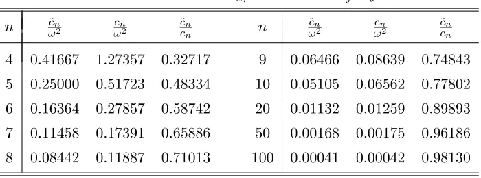
are smaller than or equal to the upper bound given in this proposition. The upper bound forc/ω2 is of the order 4/n2. An idea of how accurate our approximation of the boundary value is, can be found in Table1. In this table,cndenotes the highest value for the
coupling strengthc for which βn and hence all theβj’s are positive. These values can be found
by solving equation (20) numerically to c. The boundary value as proposed in Proposition1 is denoted by ˜cn.
Table 1. Critical valuescn/ω2in the caseλj=j−1
n ˜cn
ω2 ωcn2 cc˜nn n ωc˜n2 ωcn2 cc˜nn
4 0.41667 1.27357 0.32717 9 0.06466 0.08639 0.74843 5 0.25000 0.51723 0.48334 10 0.05105 0.06562 0.77802 6 0.16364 0.27857 0.58742 20 0.01132 0.01259 0.89893 7 0.11458 0.17391 0.65886 50 0.00168 0.00175 0.96186 8 0.08442 0.11887 0.71013 100 0.00041 0.00042 0.98130
For example, ifn= 8, all βj’s will be positive if the coupling strength c < 0.11887ω2. The
Constant interaction. The problem of finding a boundary value for the coupling strengthc so that all theβj’s are positive was discussed for constant interaction in [10]. The authors propose
an estimation of the upper bound for the coupling strength. Moreover, for n = 4, . . . ,21 they give exact values of this upper bound [10, Table 1, page 22].
4.2 The osp(1|2n) solution
Apart from the solution in terms of generators of the Lie superalgebra gl(1|n), we can also express a class of solutions of (15) by means ofosp(1|2n) generators. It is known (see [16]) that this Lie superalgebra is generated by a set of 2nparaboson operators b±j (j = 1,2, . . . , n) that satisfy the relations
{bξj, bηk}, bǫl
= (ǫ−ξ)δjlbηk+ (ǫ−η)δklbξj. (21)
In these triple relations,j, kandlare elements from the set{1,2, . . . , n}andη, ξ, ǫ∈ {+,−}(to be interpreted as +1 and −1 in the algebraic expressions (ǫ−ξ) and (ǫ−η)). The elementsb±j are the odd elements of the superalgebra, while the even elements are formed by taking anti-commutators {bξj, bηk}.
Using the relations (21) it is then easy to check (see also [11]) that the operators a−j =b−j , a+j =b+j ,
with j= 1,2, . . . , n indeed satisfy equation (15). The Hamiltonian (9) then takes the following form:
ˆ H =
n
X
j=1
~
2
q
ω2+cλ
j{a+j, a−j }=~
n
X
j=1
q
ω2+cλ
jhj, (22)
where we have introduced the notation hj ={a+j , a−j}/2 ={b+j, b−j}/2. The Cartan subalgebra
of osp(1|2n) is spanned by the n elements hj (j = 1,2, . . . , n).
5
The spectrum of ˆ
H
in a class of representations
In order to study the spectrum of the Hamiltonian ˆH in terms of the gl(1|n) or osp(1|2n) solutions, it is necessary to work with specific representations of those Lie superalgebras. An approach to this problem with respect to the Fock-type representations W(p) of gl(1|n) was given in [9]. Here, we will work with another type of representations V(p).
5.1 The gl(1|n) representations V(p)
Before analyzing the spectrum of ˆH, we will summarize the main features of the representa-tionsV(p) of gl(1|n). First of all, they are finite-dimensional, unitary representations. For any natural numberp, the basis vectors of V(p) are given by [18]
v(θ;r)≡v(θ;r1, r2, . . . , rn),
with θ ∈ {0,1}, ri ∈ {0,1,2, . . .} and θ+r1 +· · ·+rn = p. The dimension of the vector
space V(p) equals
p+n−1 n−1
+
p+n−2 n−1
in which both terms represent the number of basis vectors forθ= 0 andθ= 1 respectively. The action of thegl(1|n) generators on these basis vectors can be determined [18]. We will give the actions of the diagonal elementse00 and ekk since only these actions will be needed to find the
spectrum of the Hamiltonian: e00v(θ;r) =θv(θ;r), ekkv(θ;r) =rkv(θ;r).
In terms of the gl(1|n) generators, the Hamiltonian takes the form (19):
ˆ H =~
βe00+
n
X
j=1
βjejj
.
Clearly, looking at the actions of the elements e00 and ekk, the vectors v(θ;r) are eigenvectors
for ˆH: ˆ
Hv(θ;r) =~E
rv(θ;r),
where the eigenvalues~E
r are determined by
Er =βp−
n
X
j=1
q
ω2+cλ
jrj. (23)
This can be established by noting that
β =
n
X
j=1
βj =
1 n−1
n
X
j=1
q
ω2+cλ
j
and by using the fact that θ+r1+· · ·+rn=p.
In the case where there is no coupling (c= 0), all theβj’s become the same. It follows that
βj =ω/(n−1) and β =nω/(n−1). In this case, we thus see that the eigenvalues of ˆH are
~ω
p n−1 +θ
.
So in fact, there are two eigenvalues. The lowest one, for θ= 0, has multiplicity p+nn−−11
. The highest eigenvalue has multiplicity p+n−n−12
.
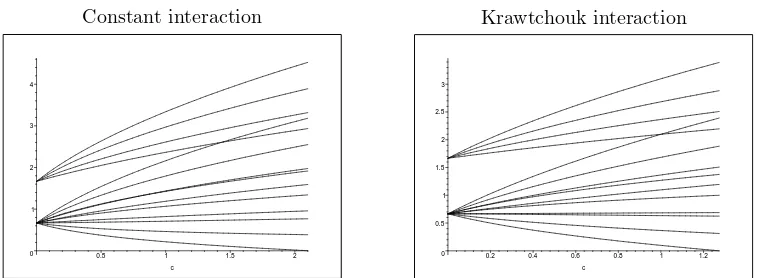
Our main interest lies in the weak coupling case, where 0< c < cn. The energy levels are
easily computed through equation (23). The result for n = 4, p = 2 and ω = ~ = 1 can be seen in Fig. 1, where we have chosen to compare the systems with constant and Krawtchouk interaction.
Both figures look quite similar, but there are some differences. We see that in general all eigenvalues are different, but for specific values of csome of the energy levels cross each other. For these values ofc, the multiplicity of some of the eigenvalues is higher than 1. In the constant interaction case, we see that energy levels can cross if we restrict ourselves to, say, θ= 0. Also, note that there are indeed only two eigenvalues in the case without coupling (c= 0).
The figure also suggests that the lowest energy level tends to zero as the coupling strength reaches cn. In order to prove this, we need to know the lowest energy level. First, we note
that βn ≤βj for all j as soon as λn ≥λj for allj. We can always choose λn to be the largest
eigenvalue, so we can assume that βn is the smallest of all βj. Next, the formula
Er =βθ+
n
X
j=1
Constant interaction
0 1 2 3 4
0.5 1 1.5 2
c
Krawtchouk interaction
0 0.5 1 1.5 2 2.5 3
0.2 0.4 0.6 0.8 1 1.2 c
Figure 1. Spectrum of the Hamiltonian (19) in the gl(1|n) representation V(p) for n= 4, p= 2 and
ω=~= 1, as a function of the coupling constantc. The left figure belongs to the system with constant interaction, where the λj are given by equation (12). The right figure represents the Krawtchouk case, withλj=j−1.
gives the energy levels as a sum of p terms. Thus, the lowest energy level arises when all p terms are equal to βn. The definition ofcn tells us thatβn= 0 for c=cn, so the lowest energy
level pβn tends to zero whenc approachescn.
5.2 The osp(1|2n) representations V(p)
We will also take a look at the (infinite-dimensional) representations V(p) of osp(1|2n), with lowest weight (p2, . . . ,p2). Such a representation is a unitary, irreducible representation (unirrep) if and only if p∈ {1,2, . . . , n−1} orp > n−1 [17, Theorem 7]. In literature, where osp(1|2n) is related to the n-paraboson algebra, the parameter p is sometimes referred to as the order of the parastatistics. A basis for the representations V(p) was given in [17], and consists of all Gelfand–Zetlin patterns for partitions of length at most n. These GZ-vectors have the following form:
|m)≡ |m)n≡
m1n · · · mn−1, n mnn
m1, n−1 · · · mn−1, n−1 ..
. . .. m11
≡
[m]n |m)n−1
.
The top line of the GZ-vectors is any partition into at most pparts, where p is the label of the representation. This partition is denoted by [m]n. For basic information about partitions, we refer to [19]. The other elements of the GZ-vectors, denoted by |m)n−1 satisfy the betweenness conditions
mi,j+1 ≥mij ≥mi+1,j+1, 1≤i≤j≤n−1.
The actions of theosp(1|2n) generators on these basis vectors are known [17]. In particular, the action of the diagonal elements hj is given by
hj|m) =
p 2 +
j
X
r=1
mrj−
j−1
X
r=1
mr,j−1
!
|m).
The Hamiltonian of the system in terms ofosp(1|2n) generators was given by equation (22):
ˆ H =~
n
X
j=1
q
ω2+cλ
From the action of the diagonal elements hj it is clear that the vectors |m) are eigenvectors of
the Hamiltonian. We can write ˆ
H|m) =~Em|m),
in which Em stands for
Em = n
X
j=1
q
ω2+cλ
j
p 2 +
j
X
r=1
mrj−
j−1
X
r=1
mr,j−1
!
. (24)
In the case without coupling (c= 0) we see that the eigenvalues simplify significantly and they can be written in the form
~ω np 2 +
n
X
r=1
mrn
!
.
The summation in this expression is in fact the weight of the partition [m]n. This weight can be any positive integerk, which we shall call the height of the eigenvalueEk(p). This means that forc= 0 there is an infinite amount of eigenvalues, that can be written as
Ek(p)=~ωnp 2 +k
, k= 0,1,2, . . . .
The multiplicity µ(Ek(p)) of each eigenvalue can be determined with the help of some theoretical arguments. First of all,µ(Ek(p)) will be equal to the total number of GZ-vectors with a partitionν in the top row, whereνis any partition ofkinto at mostpparts. Letν′be the conjugate partition of ν [19]. It is known (see for example [20, Section 4.6]) that the representation of gl(n) that is labelled by the partition ν has dimension νn′
, where we have used the generalization of the binomial coefficient for a partition [19, page 45]. This is defined by
X ν
= Y
(i,j)∈ν
X−c(i, j) h(i, j) ,
wherec(i, j) =j−iandh(i, j) =νi+νj′−i−j+ 1 are the content and the hook length of (i, j)
respectively. So for a given partition ν, the number of GZ-patterns that have ν in the top row equals νn′
. This implies that the multiplicity of each eigenvalue is equal to
µ(Ek(p)) = X
ν,|ν|=k, l(ν)≤⌈p⌉
n ν′
. (25)
The ceiling function ⌈p⌉ is used to cover the cases where n−1 < p < n. So we have found that the energy levels for c = 0 are equidistant with spacing ~ω and the multiplicities of the eigenvalues can be computed through equation (25).
In the case with actual coupling (c 6= 0) the eigenvalues can be found by equation (24). Unlike the weak coupling case in the representations V(p) of gl(1|n), the multiplicities of the eigenvalues are not all equal to one. Any two basis vectors|m) and |m′) that are subject to
j
X
r=1
mrj = j
X
r=1
yield the same eigenvalue~Em. So the multiplicity of an eigenvalue~Em is equal to the number of basis vectors for which the sum of the elements on row j is equal to the sum of the elements on rowj of|m), for every j. For example, the vectors
yield the same eigenvalue. From this it is also clear that the total number of distinct eigenvalues at heightkis equal to that number forp= 1. Indeed, every vector withp >1 can be associated with a vector withp= 1 for which equation (26) holds, as can be seen in the previous example. Moreover, all eigenvalues in the casep= 1 clearly have multiplicity 1 (in the generic case when all λj are distinct). We know what the number of eigenvalues at heightk forp= 1 is, namely
X
where the default value for k = 0 is equal to 1. The latter product is nothing more than the binomial coefficient n+n−k−11
, which shows that it is an integer.
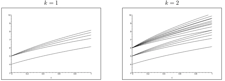
It is now clear that some eigenvalues have multiplicity greater than 1. Furthermore it is possible that some of the energy levels cross each other, just as in thegl(1|n) case. This means that for specific values ofc there are some eigenvalues for which the multiplicity is even higher. It would be inappropriate to try to compute these values of c. Let us instead look at Fig. 2, where we have plotted a part of the energy spectrum forn= 4, p= 2,ω=~= 1 andλj =j−1, to visualize things. Recall that we are dealing with an infinite spectrum. Therefore, we will only plot the spectrum up to height k, fork= 1 and k= 2. up to heightk= 1, the image on the right goes one step higher (k= 2). The total spectrum is infinite.
The eigenvalues on height 0 and 1 all have multiplicity 1 for c > 0 and they never cross. The figure on the right shows the energy values for k = 2 as well, where we both have higher multiplicities and crossing energy levels. Six of the ten distinct energy levels at height 2 have multiplicity 2.
6
Relation to canonical quantization
canonical commutation relations (CCRs)
Similarly as before, we writeA=UTDU, whereU is the orthonormal matrix with the
eigenvec-tors ofA as rows andDis the diagonal matrix with the eigenvalues ofA on the main diagonal. We define new operators ˆQ = U(ˆq1. . .qˆn)T and ˆP = U(ˆp1. . .pˆn)T. These are subject to the
same commutation relations as in equations (27) and yield a new expression for the Hamiltonian:
ˆ
We then take the linear combinations (8) of the operators ˆQand ˆP, and thus create new opera-tors a±j. The Hamiltonian can be written in terms of these new operators:
ˆ
Using the canonical commutation relations of ˆQand ˆP, one finds that the operatorsa±j satisfy the usual boson commutation relations:
a±j, a±k
= 0,
a−j , a+k
=δjk.
As before, it can also be verified that
ˆ
These are in fact the compatibility conditions derived in the general case, interpreting the system as a WQS. These CCs are also valid in the canonical case, since the CCRs imply the CCs.
We will now define the n-boson Fock space, which is equivalent to the representationV(1) of osp(1|2n). Since p= 1 represents the canonical case, we will find a correspondence between the basis vectors of V(1) and the basis vectors of the n-boson Fock space. The latter are constructed from a vacuum vector|0i, with
h0|0i= 1, a−j |0i= 0.
The other (orthogonal and normalized) basis vectors are then defined by
|k1, . . . , kni= Gelfand–Zetlin basis vectors of the representationV(1) ofosp(1|2n), generally denoted by
where we have used the notation E0 to indicate the lowest energy level. This is the lowest energy state of the system. The higher energy levels can be calculated using equation (28) in a straightforward way. This results in
ˆ
H|k1, . . . , kni=~
E0+
n
X
j=1
kj
q
ω2+cλ
j
|k1, . . . , kni.
By comparison with equation (24) for p= 1, one finds that
kj = j
X
r=1
mrj−
j−1
X
r=1
mr,j−1=mj−mj−1.
Thus we have:
Proposition 2. Then-boson Fock space and theosp(1|2n)representation spaceV(1)are equiva-lent and their basis vectors (29) and (30) are related by kj =mj−mj−1.
7
Conclusion
To conclude, we have in this paper considered the quantization of a system of harmonic oscillators as a Wigner quantum system. The quadratic coupling terms have been characterized by an interaction matrix. For such systems, the Wigner quantization procedure can be performed completely (Theorem 1), leading to a set of algebraic triple relations (11) as compatibility conditions. These relations have particular solutions in terms of generators of the Lie superalgeb-ras gl(1|n) or osp(1|2n). Then the unitary representations of these Lie superalgebras play an important role: the algebraic generators, and thus also the physical operators corresponding to observables, act in these representations. For some classes of representations, the spectrum of the Hamiltonian operator is determined explicitly, and discussed.
As leading examples throughout the paper, we consider two analytically solvable systems. The first is a classical one, describing a linear chain of harmonic oscillators coupled by a harmonic nearest-neighbour interaction. The second is a relatively new system, again describing a chain of harmonic oscillators, but this time the nearest-neighbour coupling is a “Krawtchouk coupling”. The original results in this paper are: the proof that all Hamiltonians with quadratic interac-tion terms can be reduced to an algebraic set of relainterac-tions under Wigner quantizainterac-tion (Secinterac-tion2); the conditions for the coupling strength in the case of Krawtchouk interaction for the gl(1|n) solution (Section 4); the determination and discussion of the energy spectrum for specific rep-resentations of the Lie superalgebrasgl(1|n) and osp(1|2n) (Section5). Wigner quantization is an extension of canonical quantization, so the canonical case appears as one particular solution of the various solutions allowed by Wigner quantization. For the systems under consideration here, the canonical case corresponds to the representation V(1) of the osp(1|2n) solution. This correspondence is explained in Section 6.
Acknowledgments
G. Regniers was supported by project P6/02 of the Interuniversity Attraction Poles Programme (Belgian State – Belgian Science Policy).
References
[1] Cramer M., Eisert J., Correlations, spectral gap and entanglement in harmonic quantum systems on generic lattices,New J. Phys.8(2006), 71.1–71.24,quant-ph/0509167.
[2] Regniers G., Van der Jeugt J., Analytically solvable Hamiltonians for quantum systems with a nearest-neighbour interaction,J. Phys. A: Math. Theor.42(2009), 125301, 16 pages,arXiv:0902.2308.
[3] Wigner E.P., Do the equations of motion determine the quantum mechanical commutation relations?,Phys. Rev.77(1950), 711–712.
[4] Kamupingene A.H., Palev T.D., Tsavena S.P., Wigner quantum systems. Two particles interacting via a harmonic potential. I. Two-dimensional space,J. Math. Phys.27(1986), 2067–2075.
[5] Green H.S., A generalized method of field quantization,Phys. Rev.90(1953), 270–273.
[6] Palev T.D., Wigner approach to quantization. Noncanonical quantization of two particles interacting via a harmonic potential,J. Math. Phys.23(1982), 1778–1784.
[7] Palev T.D., Stoilova N.I., Many-body Wigner quantum systems,J. Math. Phys.38(1997), 2506–2523.
[8] B lasiak P., Horzela A., Kapu´scik E., Alternative hamiltonians and Wigner quantization,J. Opt. B: Quantum Semiclass. Opt.5(2003), S245–S260.
[9] Lievens S., Stoilova N.I., Van der Jeugt J., Harmonic oscillators coupled by springs: discrete solutions as a Wigner quantum system,J. Math. Phys.47(2006), 113504, 23 pages,hep-th/0606192.
[10] Lievens S., Stoilova N.I., Van der Jeugt J., Harmonic oscillator chains as Wigner quantum systems: perio-dic and fixed wall boundary conditions in gl(1|n) solutions, J. Math. Phys. 49(2008), 073502, 22 pages,
arXiv:0709.0180.
[11] Lievens S., Van der Jeugt J., Spectrum generating functions for non-canonical quantum oscillators,
J. Phys. A: Math. Theor.41(2008), 355204, 20 pages.
[12] Cohen-Tannoudji C., Diu B., Lalo¨e F., Quantum mechanics, Wiley, New York, Vol. 1, 1977.
[13] Brun T.A., Hartle J.B., Classical dynamics of the quantum harmonic chain,Phys. Rev. D60(1999), 123503,
20 pages,quant-ph/9905079.
[14] Audenaert K., Eisert J., Plenio M.B., Werner R.F., Entanglement properties of the harmonic chain, Phys. Rev. A66(2002), 042327, 14 pages,quant-ph/0205025.
[15] Gould M.D., Zhang R.B., Classification of all star irreps ofgl(m|n),J. Math. Phys.31(1990), 2552–2559.
[16] Ganchev A.Ch., Palev T.D., A Lie superalgebraic interpretation of the para-Bose statistics,J. Math. Phys. 21(1980), 797–799.
[17] Lievens S., Stoilova N.I., Van der Jeugt J., The paraboson Fock space and unitary irreducible representations of the Lie superalgebraosp(1|2n),Comm. Math. Phys.281(2008), 805–826,arXiv:0706.4196.
[18] King R.C., Stoilova N.I., Van der Jeugt J., Representations of the Lie superalgebragl(1|n) in a Gelfand– Zetlin basis and Wigner quantum oscillators,J. Phys. A: Math. Gen.39(2006), 5763–5785,hep-th/0602169.
[19] Macdonald I.G., Symmetric functions and Hall polynomials, 2nd ed., The Clarendon Press, Oxford Univer-sity Press, New York, 1995.
[20] Wybourne B.G., Symmetry principles and atomic spectroscopy, Wiley, New York, 1970.