www.elsevier.nl / locate / econbase
Tax reform evaluation using non-parametric methods:
Sweden 1980–1991
a ,* a b
¨ ¨
Soren Blomquist , Matias Eklof , Whitney Newey
a
Department of Economics, Uppsala University, Box 513, S-751 20 Uppsala, Sweden
b
Department of Economics, Massachusetts Institute of Technology, Boston, MA, USA Received 31 July 1998; accepted 29 February 2000
Abstract
This paper evaluates the tax reform carried out in Sweden between 1980 and 1991. We use a recently developed non-parametric estimation technique to account for the labor supply responses of married prime aged males. We decompose the tax reform to study how the separate components influence hours of work, tax revenue, and income distribution. We find that the decrease in marginal tax rates stimulated labor supply but that the other parts of the reform counteracted this effect. The net increase in average desired hours of work was approximately 2%. We also find that the reform was under financed and that inequality increased. The non-parametric predictions are compared to the results based on a flexible parametric model. The qualitative results are similar, but the quantitative results are quite different. 2001 Elsevier Science B.V. All rights reserved.
Keywords: Non-parametric estimation; Labor supply; Tax revenues; Income distribution
JEL classification: C14; D31; H31; J22
1. Introduction
The Swedish tax system has during the last couple of decades been transformed in several important ways. Marginal tax rates reached a peak around 1980. However, since this system with very high marginal tax rates was combined with a
*Corresponding author. Tel.:146-18-471-1102; fax:146-18-471-1478.
¨
E-mail addresses: [email protected] (S. Blomquist), [email protected] (M. Eklof). 0047-2727 / 01 / $ – see front matter 2001 Elsevier Science B.V. All rights reserved.
system of fairly liberal rules for deductions of various forms, many economic agents could avoid the high marginal taxes by using the system of deductions in a clever way. During the eighties, there was a series of tax reforms, decreasing marginal tax rates and limiting the scope for various forms of deductions. The series of tax reforms culminated in 1991 with a large change in marginal taxes between 1990 and 1991, several types of base broadening and the introduction of separate taxation of labor and capital income.
Several motivations have been given for implementing the tax reforms. The need to reduce the negative incentive effects of high marginal tax rates on household behavior such as savings and labor supply is probably the single most important one. Another motivation was a concern that the distributional effects of the old tax system were not the ones intended. The use of deductions could in many cases lead to high income earners paying very little in taxes.
The tax reform has been a continuous and gradual process for a long period of time. We therefore have a choice of what part of this process to study. We have chosen to study the effect of the tax reform that took place between 1980 and 1991. This period is of special interest since the tax systems in these two years constitute two extremes. Marginal tax rates reached a historical high in 1980 and a
1
low in 1991. We do not cover all aspects of the tax reform but focus on four changes of large importance for individual behavior; a decrease in marginal tax rates, an increase in the VAT and payroll taxes, a change in the rules for capital
2
income taxation and deductions, and a change in the transfer system.
The major purpose of our paper is to study how the tax reform has affected desired hours of work, tax revenue, and the income distribution. We investigate the net effect of the tax reform, but also perform a decomposition so we can see the effects of its various parts. The evaluation of the reform is performed by simulations. The benchmark of the calculations is the 1980 tax and transfer system coupled with the observed distribution of gross wage rates, capital income and other socio-demographic variables in 1980. In a predefined sequence, we substitute the tax and transfer rules in the 1991 system for the corresponding rules in the 1980 system and calculate the desired hours of work, the tax revenues, and the income distribution.
The paper contains three methodological advances as compared to many earlier studies. First, we decompose the overall set of policy changes into its component effects. This is useful, since if the policy makers would like to do further reforms it is essential to know the effects of the separate instruments that together form the tax system. Second, a novel feature of this study is that we use a non-parametric labor supply function to calculate how hours of work change in response to the tax reform. Since this non-parametric function requires less stringent distributional and
1
After 1991 there have been some increases in the marginal tax rates.
2
functional assumptions this should lead to more reliable predictions than if a parametric function was used. This method is still not developed for household models. We therefore only present calculations of how hours of work change for married or cohabiting men in ages 20–60. This group constitutes a major part of
3
the labor force if measured by the part of the tax base it generates. We find that the non-parametric approach yields different predictions than those of a ‘state of the art’ parametric model. Third, behavioral responses are usually neglected in income distribution studies. In our analysis, we (partly) account for these responses and therefore we believe this study to give better predictions of the effects on income distribution.
The rest of the study is organized as follows. In Section 2, we give a stylized description of the Swedish tax reform. The motivation for using non-parametric methods and a brief description of the parametric and non-parametric supply functions are given in Section 3. In Section 4, we describe how the tax reform is decomposed and present our calculations of the effect of the tax reform on hours of work, tax revenue and income distribution. Section 5 concludes.
2. Swedish tax reforms 1980–1991
This section gives a brief presentation of the 1980 and 1991 tax and transfer systems. A more detailed description of the systems can be found in Blomquist and Hansson-Brusewitz (1990) and Blomquist et al. (1998).
2.1. Personal income taxation
The 1980 personal income tax system consisted of a progressive federal income tax and a proportional local income tax, both levied on taxable income. The taxable income was defined as the sum of labor income net of payroll taxes, capital income, an imputed rental income for owner occupied homes and other sources of income, minus deductions of various sorts. The federal income tax was highly progressive with marginal tax rates ranging from zero to 58%. The local income tax was on average 29%. Thus, the maximum (unconstrained) marginal tax rate was approximately 87%. However, to bound the marginal effects the 1980 tax system restricted the marginal tax rate at 80% for taxable income below SEK
4
174 000 and 85% for higher taxable incomes.
By 1991, the federal marginal tax rates had been reduced to 0% in low income
3
Aronsson and Palme (1998), using a parametric household model, study how labor supply, tax revenues and income distribution are affected by the tax reform. Agell et al. (1996) give a broad picture and evaluation of the tax reform.
4
All figures are deflated to the 1980 price level using a consumer price index. We use the consumer ˚
brackets and 20% in high brackets. The local tax was increased by 1.9 percentage points on average. The marginal tax rates thus ranged from zero to slightly above 50%. The federal and local taxes were levied on labor income net of payroll taxes and deductions. The other two main sources of income (capital income and implicit income of owner occupied homes) were taxed separately from labor income. Incomes from capital were taxed at a uniform rate of 30%. A capital deficit implied a tax reduction but it did not influence the marginal tax rate on labor income. The tax on owner occupied homes was proportional at 1.2% of the
5
ratable value of the house.
2.2. Indirect taxes
The net tax revenue for the government was predicted to be reduced by the tax and transfer reform. To compensate for this, the VAT and the payroll tax were increased. The payroll tax increased from 35.25% in 1980 to 37.47% in 1991, measured as a percentage of the wage rate net of pay roll taxes. Although a part of the payroll tax could be considered as an insurance fee, we have chosen to treat it as a pure tax. Simultaneously with a broadening of the VAT base, the general VAT rate increased from 21.34% in 1980 to 25% in 1991, measured as a percentage of the price exclusive of VAT. However, some commodities and services that were excluded from VAT in 1980 became taxed in 1991. This base broadening gives us reason to use an average VAT on a consumption bundle as an approximation of the net effect of the increased VAT and the base broadening. In practice, we define the average VAT as the aggregate tax revenue from VAT divided by the aggregate private consumption (excluding the VAT liability). The average VAT equaled 12.8 and 16.5% in 1980 and 1991, respectively.
2.3. Transfer system
The basic design of the housing allowance schemes was similar in the 1980 and 1991 transfer systems. First, the maximum allowance was calculated based on the housing costs and the family composition. Next, the allowance was reduced depending on the household income and family wealth. One noteworthy difference between the systems is the importance of family composition relative to housing costs. In 1980, the allowance increased with the number of children in the household. The 1991 system made a difference between households with and without children, but the allowance did not increase with the number of children. The importance of housing costs were decreased in the reform, reducing the
5
Simultaneously with the reform of the property taxation, the ratable values of the house were adjusted. We have taken this into account by calculating the market value of the house (ratable value in 1980 times the (national) purchase price index in 1980) and then dividing the market value with the
¨
maximum compensation from 80% of the housing costs to approximately 65%. The rate at which the allowance was reduced as the household’s income increased also differed across the systems and family compositions. The reduction rate in 1980 varied between 15 and 24%. In 1991, the reduction rates varied between 10 and 30% depending on family composition. The construction of the allowance generated non-convexities in both the 1980 and the 1991 budget constraints. The transfer reform also included a more generous child allowance, which was independent of the household’s income.
2.4. Effects on budget constraints
It is helpful to make the following definitions. The pre-payroll wage rate is defined as the (total) hourly wage rate paid by the employer, i.e. before payroll and income taxes. The gross wage rate is conventionally defined as the wage rate net of payroll taxes but before income taxes. The net wage rate is defined as the wage rate net of payroll and income taxes and transfers. All wage rates are measured in terms of the consumer price level, which includes the VAT.
In the previous paragraphs, we pointed out the major differences between the 1980 and 1991 tax- and transfer systems. In order to evaluate the effects of these differences on the budget constraints we make the following assumptions:
A1. The pre-payroll wage rate in nominal terms is unaffected by the changes in
6
the tax system.
A2. The producer prices in nominal terms are unaffected by the changes in the
7
tax system.
A3. The tax and transfer system parameters are constant in nominal terms. A4. Individuals consume all their net income.
The heterogeneity of individuals makes it difficult to illustrate the overall effect on the budget constraint of the reform; different individuals are affected differently by the reform. For a given combination of the variables that determine the budget constraint, we can plot the marginal effects against hours of work. The question is how to choose this combination. We have constructed three synthetic individuals
8
with pre-payroll wage rates equal to SEK 27, 54 and 108, respectively. The other variables that are of importance for the shape of the budget constraint are constructed as sample averages for individuals with pre-payroll wage rates within
6
This assumption implies that the increase in the pay roll tax described above will lead to a decrease in the gross wage rate of 1.6%.
7
This assumption implies that the consumer price level will increase by 3.3% due to the changes in the VAT rules.
8
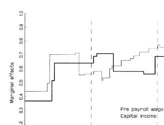
Fig. 1. Marginal effects faced by an average paid individual.
plus minus SEK 10 of the three wage rates. This enables us to present the general picture of the effects faced by low, average and high paid types taking account of the correlation between the wage rate, capital income, income of spouse and socio-demographics.
In Fig. 1, we illustrate the marginal effects faced by an average paid person for the 1980 and 1991 tax and transfer systems. The imputed capital income used in this calculation is SEK 210,900. The vertical dashed lines indicate 1040 and 2080 annual hours of work, respectively. Note that we present the total marginal effects, i.e. we include the effects of the payroll tax, the VAT, and the tax and
9
transfer system in the calculations of the marginal effects. This explains why we report higher marginal effects than some earlier studies that only report the marginal tax rates.
9
The marginal effect, m(huz), is defined as:
12t(huz)
]]]]] 12
(11VAT )(11PRT )
where h denotes hours of work, z a vector of individual characteristics that determine the shape of an individual’s budget constraint,tis the marginal tax rate including the effects from the transfer system,
VAT is the value added tax rate, and PRT is the payroll tax. The VAT is measured as a percentage of the
Fig. 1 indicates that, for an average paid individual, the marginal effects differ across the two tax- and transfer systems The differences presented here are not as large as has been suggested by other studies. The ‘humps’ between 500 and 1500 hours originate from the construction of the housing allowance systems and reflect the reduction of the allowance. One important difference between the two systems is the effects of a capital deficit on the marginal effects. In the 1980 system, a capital deficit shifts the marginal effects rightwards while the same capital deficit in the 1991 system leaves the marginal effects unchanged beyond some point on the x-axis. To the left of this point, all tax liabilities are reduced to zero due to the tax reduction of capital deficits.
In Table 1, we present the calculated marginal effects at part and full working
10
time for the three synthetic individuals defined above. It should be noted that these numbers are just points on discontinuous functions of the type presented in Fig. 1. Hence, small changes in the pre-payroll wage rate or the hours of work may cause an individual to face another tax segment and consequently another marginal tax rate. We also repeat that the capital income and socio-demographics covary with the pre-payroll wage rate according to the joint distribution in our 1980 sample.
The table indicates that the marginal effects have decreased at full time hours for all three types. The decrease is less than ten percentage points for low and average paid persons, but almost 20 percentage points for high paid individuals. The changes at part time hours differ in both size and sign. For low paid types, the marginal effect was reduced by seven percentage points, whereas the marginal effect increased by eight points for the average paid and by 16 points for the high paid type.
In Table 2, we present the net income, i.e. income net of tax and transfers, for different wage rates and hours of work under the two tax systems. As before, we let capital income and socio-demographics covary with the pre-payroll wage. We also present the percentage difference between the net income in the two tax- and transfer systems.
Table 1
Marginal effects at part and full time hours of work (in %) Pre-payroll Part time Full time wage rate (1040 h) (2080 h)
1980 1991 1980 1991
At a slightly lower value of hours of work, the marginal effects are close to 70%.
10
Table 2
Net incomes at part and full hours of work
Pre-payroll Part time (1040 h) Full time (2080 h) wage rate
1980 1991 Diff. % 1980 1991 Diff. %
27 50 102 56 081 12 62 007 64 305 4
54 65 015 72 028 11 87 190 92 860 7
108 88 787 90 716 2 113 008 126 932 12
The net income increases at all tabulated wage rates and working hours due to the reform. The increase is most pronounced for low and average paid persons that are part time workers (11–12%) and for full time workers with high wage rates (12%).
3. The non-parametric and parametric supply functions
Ideally, we would like to estimate a household model. However, the non-parametric procedure is newly developed and has not been generalized to handle that case. Some scholars argue that female hours of work are more responsive to changes in taxes than hours of work for men and that it therefore might be of larger interest to study the labor supply response of women. We do not share this view. Blomquist and Hansson-Brusewitz (1990), estimating parametric models for males and females separately, found that working males and females react roughly
11
in the same way to changes in budget constraints. It is true that the participation decision is more important for women than for men. However, given that the labor force participation rate in Sweden in 1980 was above 80% for married women, this is less important in Sweden than in many other countries. Since men in general have higher wages than females, we believe it is of larger interest to study the response of men if we are interested in effects on tax revenue and distributional
12
effects. When studying the labor supply of men we take the hours of work of the
13
spouse as given.
11
Since average female hours is much lower than average male hours this implies that the reported elasticity figure is higher for women.
12
According to the Level of Living survey from 1980, the average gross wage rate was about 33% higher for working married men than for working married women.
13
3.1. Data source
Three waves of the Swedish ‘Level of Living’ survey, with data from 1973,
14 ,15
1980 and 1990, were used for the estimation. Only data for married or cohabiting men in ages 20–60 are used. Farmers, pensioners, students, those with more than 5 weeks of sick leave, those liable for military service and self employed are excluded. This leaves us with 777 observations for 1973, 864 for 1980, and 680 for 1990. The fact that data from three points in time are pooled has the obvious advantage that the number of observations increases. Another important advantage is that there is a variation in budget sets that is not possible with data from just one point in time. The tax systems were quite different in the three time periods, which generates a large variation in the shapes of budget sets. The tax systems for 1973 and 1980 are described in Blomquist (1983) and Blomquist and Hansson-Brusewitz (1990). The tax system for 1990 is described in Appendix A of Blomquist and Newey (1999). Housing allowances have over time become increasingly important. For 1980 and 1990, we have therefore included the effect of housing allowances on the budget constraints.
3.2. Non-parametric supply function
Parametric estimation methods impose further restrictions than those implied by economic theory. These restrictions can be particularly severe when estimating labor supply functions generated by non-linear budget constraints. Blomquist and Newey (1999) therefore develop a non-parametric method to estimate labor supply functions generated by non-linear, or piece wise linear, budget constraints. In this paper, we will adopt the non-parametric function presented in Blomquist and Newey (1999). We refer the interested reader to that paper for details of the procedure and description of its properties. Below we only give a brief summary of the estimation procedure.
The method is based on the idea that labor supply can be viewed as a function of the entire budget set, so that one way to account non-parametrically for a non-linear budget set is to estimate a non-parametric regression where the variable in the regression is the budget set. In the special case of a linear budget constraint, this estimator would be the same as non-parametric regression on wage and non-labor income, since these two numbers characterize the budget set. The method would then be similar to the one used in Hausman and Newey (1995).
Non-linear budget sets will be characterized by more numbers than two, for example for piece wise linear budget sets by slopes and intercepts of the linear
14
The data are briefly described in Blomquist (1983), Blomquist and Hansson-Brusewitz (1990) and Blomquist and Newey (1999).
15
segments. The Swedish tax and transfer system in 1980 generated budget constraints consisting of up to 27 segments. To represent such a constraint would require 54 numbers! Non-parametric estimation using actual budget constraints consisting of 27 segments would require huge amounts of data. A practical estimation procedure must therefore reduce the dimensionality of the problem so that a budget constraint can be represented with just a few numbers.
Blomquist and Newey (1999) suggest a two-step estimation procedure. In the first step, each actual budget constraint is approximated by a continuous budget
16
constraint consisting of three piece wise linear segments. Denote the slopes of these segments by wi, and the intercepts by y , ii 51, 2, 3. The kink points of the budget constraint can be expressed in terms of the slopes and intercepts of the linear segments. The first kink point can be expressed as l15( y22y ) /(w1 12w )2
and the second as l25( y32y ) /(w2 22w ). It is useful to define the following3
functions of the kink points, slopes, and intercepts: dy5l ( y1 22y )1 1l ( y2 32y )2
and dw5l (w1 22w )1 1l (w2 32w ). In the second step series estimation is2
performed, using the approximated budget constraints as data.
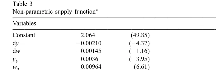
Expected hours of work is an unknown function of the slopes, intercepts and kink points of the piece wise linear budget constraint. Two types of approximating functions that can be used in constructing series estimators are power series and regression splines. In our case, we use power series. That is the approximating function will consist of powers of pairs of kink points, intercepts and slopes. To make use of the non-parametric flexibility of series estimators it is important to let the data determine what terms should be included. In that way, the non-parametric feature of the estimator becomes active. We use a cross-validation criterion to decide what terms that should be included. The exact form of this criterion is given in Blomquist and Newey (1999). In practice, a large number of functions are estimated, where each function is a particular power series of the kink points, wages, and virtual incomes. The particular form that yields the highest cross-validation criterion turned out to be a fairly simple form containing only one quadratic term. This function is presented in Table 3. This function might look as a parametric function, but it is in fact fully non-parametric. This is because the cross-validation criterion has been used to choose what terms to include in the
17
series approximation.
The estimation procedure allows for random preferences and measurement error in hours of work. Two basic assumptions for the procedure to work are that the
16
Blomquist and Newey (1999) also try approximations with four-piece wise linear segments. However, the cross-validation criterion indicates that the approximation with three segments is preferable.
17
Table 3
Dependent variable: hours of work in thousands; income in thousands of SEK; t-values in parentheses. The delta method was used to calculate the t-values for the elasticities.
random preference term is uncorrelated with the budget constraints and that the expectation of the measurement error is zero given any budget constraint. Blomquist and Newey (1999) provide asymptotics for the estimator and also
18
present results from Monte Carlo simulations. The simulations indicate that the non-parametric procedure performs quite well in terms of predicting the effect of tax reform on average hours of work.
3.3. Parametric supply function
We also estimate a parametric labor supply function similar to the random preference model described in Blomquist and Hansson-Brusewitz (1990). To perform this estimation we have convexified the budget constraints for data from 1980 and 1990. There is a wide choice of parametric functions to estimate. A labor supply function linear in the wage rate and non-labor income has been used extensively in previous labor supply studies. It can therefore be of interest to estimate this parametric form. However, this functional form is quite restrictive. We therefore also estimate a more flexible form advocated by Blundell et al. (1998). This function is linear in the logarithm of the wage rate and the ratio of non-labor income and the wage rate. It turns out that the predictions of the effect of tax reform on average hours of work are very similar for the two functions. We
18
19
therefore only show the more flexible function here. Results for the linear specification are presented in Blomquist et al. (1998). The estimated function is
20
shown in Eq. (1) with the t-values given in parenthesis beneath each coefficient.
23 22 23
Here h denotes hours of work in thousands, w the wage in SEK and y income in thousands of SEK. AGE denotes a dummy variable taking on the value 1 for ages 46–60 and zero otherwise. NC denotes the number of children under age 20 living at home. Both these variables are insignificant. The symbolsshandse denote the standard deviations of an additive random preference term and an optimization / measurement error, both normally distributed with mean zero. The wage and income elasticities, E and E , are evaluated at the mean of the net wage rates andw y
virtual incomes from the segments where individuals observed hours of work are
21
located. Of course, the wage and income elasticities are summary measures of how the estimated functions predict how changes in a linear budget constraint affect hours of work. None of the budget constraints used for the estimation are linear and we actually never observe linear budget constraints. It is therefore of larger interest to see how the predictions differ between the parametric and non-parametric labor supply functions for discrete changes in non-linear budget constraints. Such calculations are given below.
4. Simulation results
The Swedish tax reform consists of many different parts. If the policy makers would like to do further changes in the tax system it would be of value to know the effects of the various components of the tax reform. Which changes in the past
19
Of course, one could argue that the form suggested by Blundell et al. also is too restrictive and that our results are biased because of this. However, it is our impression that the form we use is considered to be one of the more flexible ones. Also, whatever parametric form we try one could always argue that we have chosen a too restrictive form. We can never know whether we have chosen a parametric form flexible enough. This is, we believe, an indication of one of the advantages of using a non-parametric technique.
20
The variance–covariance matrix for the estimated parameter vector is calculated as the inverse of the Hessian of the log-likelihood function evaluated at the estimated parameter vector. We have had to resort to numerically calculated derivatives. It is our experience that the variance–covariance matrix obtained by numerical derivatives gives less reliable results than when analytic derivatives are used.
21
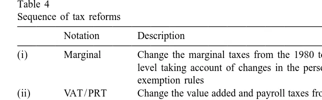
Table 4
Sequence of tax reforms
Notation Description
(i) Marginal Change the marginal taxes from the 1980 to the 1991 level taking account of changes in the personal exemption rules
(ii) VAT / PRT Change the value added and payroll taxes from the 1980 to the 1991 levels
(iii) Capital Change the capital income tax rules and the rules for taxation of homes
(iv) Transfer Change the housing allowance and child allowance rules
has stimulated labor supply most. What changes work in the opposite direction? What changes increase tax revenue? What changes decrease tax revenue? As far as we know this is the first study that makes a detailed decomposition of the tax reform.
The decomposition can be made in several ways. One would be to follow the exact chronological order in which the reform has taken place. However, if we follow this route we intertwine decreases in marginal tax rates, base broadening, restrictions in rules for deductions, and changes in the transfer system. We believe this will blur the picture. Instead, we have chosen to use the sequence presented in Table 4.
We calculate the effect of a reform, given the previous changes. This implies that the picture of the effect of the various parts of the reform that we obtain depends on the sequence in which we introduce the various parts of the reform. A motivation for the chosen sequence is as follows. The decrease in marginal taxes was one of the cornerstones in the tax reform and many perhaps regard this as the quintessence of tax reform, which motivates its place first in the sequence. To finance the decreased marginal taxes the increase in indirect taxes and the separation of capital and labor income follows next. The changes in the housing and child allowance systems were designed so as to correct for unwanted distributional effects of other changes in the tax system, so it is natural to place this part of the reform last in the sequence.
4.1. Desired hours of work
We use the distribution of gross wage rates and non-labor incomes in the 1980
22
data set as the basis for our calculations. For each observation in the 1980 data
22
set, we use the gross wage rate, the non-labor income and the socio-demographics in combination with the appropriate tax and transfer system to construct a budget set. This budget set is then approximated by a budget constraint consisting of three continuous piece wise linear segments. Finally, we use the non-parametrically estimated labor supply function to calculate the expected desired hours of work. We would have liked to account for labor supply changes of spouses. However, since the estimation procedure is not yet developed for households we are forced to treat their labor supply as fixed. A rather weak justification for this assumption is that a study of the tax reform by Aronsson and Palme (1998), estimating a parametric household model, found that the net effect of the tax reform on spouses’ hours of work was close to zero due to two counteracting effects on the female labor supply. In the simulations, we fix the labor supply of the spouse at observed hours in the 1980 data set. Nevertheless, in our calculations we take account of how the changes in the tax and transfer rules affect the after tax income of the spouse, which affects the intercept of the husband’s budget constraint.
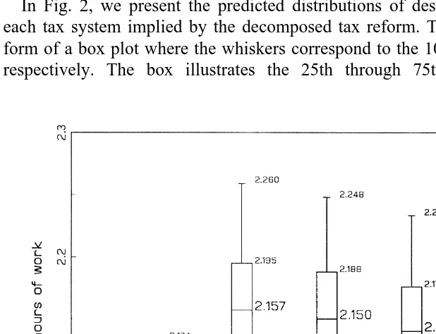
In Fig. 2, we present the predicted distributions of desired hours of work for each tax system implied by the decomposed tax reform. The illustration is in the form of a box plot where the whiskers correspond to the 10th and 90th percentile, respectively. The box illustrates the 25th through 75th percentiles and the
horizontal bar marks the sample median. The numbers to the right of the box give the values of the corresponding hours of work The five boxes are generated by the (cumulative) introduction of the defined reforms as indicated by the labels on the horizontal axis. The vertical axis corresponds to desired hours of work.
The box plot shows that the decrease in marginal tax rates lead to a substantial increase in hours of work. The median increases from 2082 hours per year to 2157 hours. The marginal tax reform also increases the dispersion of hours from an interquartile distance of 37 hours in 1980 to 64 hours with the lower marginal rates. The other reforms in the sequence all reduce desired hours of work by less than 1% each. In Table 5 we present the sample means for desired hours and also the percentage change w.r.t. the sample mean of the 1980 tax system. Since the distributions are skewed towards the right the means are higher than the medians. The table shows that average desired hours of work increases by 3.9% due to the marginal tax reform but that the hours of work decreases by approximately 0.3, 0.4, and 0.9 percentage points as we introduce the increased indirect taxes, the separation of capital taxation and the new transfer system. The net increase in average desired hours of work is approximately 2.2%.
4.2. Pre-payroll wage and labor supply effects
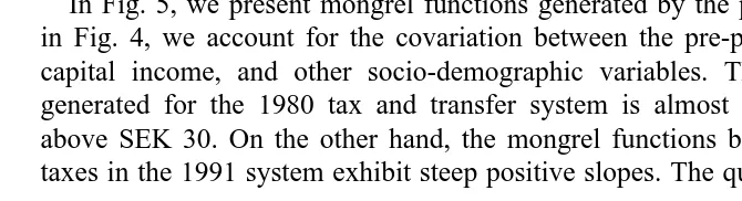
The mongrel function, defined and discussed in Blomquist and Hansson-Brusewitz (1990), gives desired hours of work as a function of the pre-payroll wage rate, non-taxable and taxable non-labor income, and socio-demographic variables, given a specific income tax system. Hence, each tax system generates a separate mongrel function. Another way to illustrate the effect of the various components of the reform is therefore to graph the mongrel functions for each of the tax systems defined by the sequence in Table 4. In Fig. 3, we show mongrel curves where non-labor income and the socio-demographic variables have been set to the sample averages and the pre-payroll wage rate varies from SEK 30 per hour to SEK 80. This interval corresponds to the 2nd through 9th deciles in the observed distribution of pre-payroll wage rates. The solid thin line illustrates the mongrel function generated by the 1980 tax and transfer system. The thicker solid line shows the function generated by the 1991 tax system. The mongrel functions
Table 5
Estimated means of desired hours of work
1980 Marginal VAT / PRT Capital Transfer
Mean 2.093 2.174 2.167 2.158 2.139
Fig. 3. Mongrel supply functions; non-labor income and socio-demographics constant and set to sample averages.
generated by the intermediate tax and transfer systems are illustrated by the
23
dashed, dashed-dotted, and connected lines, respectively.
We note that the mongrel function generated by the 1980 tax and transfer system has a negative slope for pre-payroll wage rates between SEK 40 and SEK 80. This feature is also found in Blomquist and Hansson-Brusewitz (1990) and is due to the high progressiveness in the Swedish 1980 tax system. As we introduce the marginal tax rate reform, the mongrel function shifts upwards and has a positive slope at all wage rates. A comparison of the mongrel functions shows that the desired hours of work increases as a response to the decreased marginal tax rates. The increase in the indirect taxes, as well as the separation of labor and capital income taxation, reduce desired hours of work at all wage rates. Finally, the introduction of the 1991 transfer system reduces hours of work at all wage rates, in
23
particular at low levels. This implies that the positive slope of the mongrel function becomes steeper as compared to the previous cases. The net effects of the tax and transfer reform are that individuals with low wage rates decrease their desired hours of work, and that individuals with wage rates above the average increase their desired hours, as compared to the pre-reform situation.
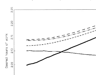
We also calculate the mongrel functions in an alternative way where we let the capital income and the socio-demographic variables covary with the pre-payroll wage. To impose the relevant covariation we use the observed joint distribution of all relevant individual characteristics and the pre-payroll wage rate in the 1980 sample.
We want to emphasize the following methodological distinctions between Figs. 3 and 4. First, as already mentioned, the underlying distribution of the individual characteristics differs across the figures. Second, the distribution of observations over the wage rates differs across the figures. In Fig. 3 the distribution of pre-payroll wage rates are uniformly distributed over the horizontal axis. In Fig. 4, however, we have used the observed distribution of pre-payroll wage rates, which implies that there are very few observations in the left tail of the mongrel functions and therefore the precision of the functions is low in the left tail.
Fig. 4 gives a somewhat different picture of the effects of the tax reforms than Fig. 3 does. For low pre-payroll wage rates, the net effect of the tax reform on hours of work is negligible or slightly positive. This is in contrast to the results in Fig. 3. For high pre-payroll wage rates, the result holds that the reform increases the desired hours work considerably. There is no single covariate that causes the difference between Figs. 3 and 4. The fact that the capital deficit is larger at higher wage rates is important, but other covariates are also of importance. The final conclusion is that the reform leads to an increase in average desired hours of work. Individuals with high wage rates were affected more by the reform than low paid individuals.
4.3. Parametric predictions of desired hours of work
To illustrate some of the differences between parametric and non-parametric predictions we duplicate part of the analysis in the previous section with the modification that we use a parametric model to predict desired hours of work. The parameters are found in Eq. (1). Since this is a random preference model, we need to draw several random numbers for each observation in order to calculate expected desired hours of work. The results presented in Table 6 and Fig. 5 are based on the average of 100 replications. In Table 6 we present the simulated distributions of desired hours of work. These results can be compared to Fig. 2 and Table 5
The parametric model predicts a larger increase in hours of work than the non-parametric model. The percentage increases in sample means are about twice as high and the interquartile distance is considerably larger than estimated by the non-parametric model.
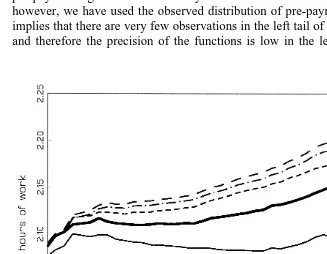
In Fig. 5, we present mongrel functions generated by the parametric model. As in Fig. 4, we account for the covariation between the pre-payroll wage rate, the capital income, and other socio-demographic variables. The mongrel function generated for the 1980 tax and transfer system is almost horizontal for wages above SEK 30. On the other hand, the mongrel functions based on the marginal taxes in the 1991 system exhibit steep positive slopes. The qualitative results from
Table 6
Distribution of desired hours of work (parametric model)
Percentile 1980 Marginal VAT / PRT Capital Transfer
Mean 2.084 2.215 2.204 2.195 2.182
%D 0.0 6.3 5.8 5.4 4.7
90th 2.151 2.300 2.291 2.277 2.275
75th 2.115 2.247 2.236 2.219 2.214
50th 2.080 2.206 2.197 2.189 2.178
25th 2.047 2.172 2.161 2.158 2.137
Fig. 5. Parametric predictions of hours of work by decomposed reform.
the non-parametric model holds, i.e. the marginal tax reform encourage labor supply, and the increased indirect taxes, the separation of capital and labor income taxation, and the new transfer system all reduce desired hours of work.
Comparing the predictions of the non-parametric and parametric models, we conclude that the qualitative effects on hours of work are similar but the magnitude of the variation is much larger in the parametric model. The percentage increase in average hours of work by introducing the 1991 marginal tax rates is approximately 6.3% compared to 3.9% predicted by the non-parametric model. The net percentage increase is 4.7% by the parametric model and 2.2% by the non-parametric. Another notable difference is the distribution of hours of work, where the non-parametric model implies a less dispersed distribution of expected hours of work.
4.4. Tax revenue
Table 7
Average tax revenue from households
Tax Non-parametric Parametric Fixed
source model 1991 supply 1991
1980 Marginal VAT / PRT Capital Transfer
PRT 43 986 45 393 46 893 46 737 46 442 47 107 45 545
Transfer 3596 3554 3578 3579 5766 5723 5764
% 0 21 21 20 60 58 60
Net Rev. 93 355 84 945 87 266 88 535 87 576 89 237 85 336
% 0 29 27 25 26 24 29
categories, where the first is associated with the payroll taxes, the second with personal income taxes, such as labor income taxes, capital taxes and taxes on
24
property. The third category refers to tax revenue from the VAT.
Table 7 presents the results from the simulations. In the first row, we present the average tax revenue from payroll taxes. The second row shows tax revenue from personal taxation of labor income, capital income, and taxes on property. The third row gives the revenue from VAT and the fourth presents the average transfers, i.e. housing and child allowances. The bottom row gives the net tax revenue. The number just below each row gives the percentage increase in the revenue from the indicated source w.r.t. the 1980 tax and transfer system. The column titles indicates the introduced reform and the last two columns gives the final results predicted by the parametric model and a model that ignores the labor supply effects. In the latter case we use the non-parametrically estimated distribution of desired hours of work based on the 1980 tax and transfer system.
Table 7 shows some interesting features of the tax reform. First, we notice that the importance of the personal income taxes are reduced relative to the indirect taxes. In 1980, the income tax accounted for approximately 46% of tax revenue (excluding transfers). In the 1991 system, this figure is reduced to 41%. The table also indicates that the marginal tax reform generated a financial deficit of approximately 9% and that the subsequent tax reforms only partly compensated for this deficit. The increased indirect taxes reduced the deficit to 7%. The capital tax reform further reduced the deficit to 5%. The transfer reform increased the transfer payments by 55% on average, which increased the deficit to 6%, which is also the net deficit of the tax and transfer reform.
24
Table 8
Gini coefficients on net incomes
1980 Marginal VAT / PRT Capital Transfer
Non-parametric
Heads 0.111 0.158 0.159 0.166 0.155
Equivalent 0.135 0.156 0.156 0.157 0.147
Parametric
Heads 0.113 0.159 0.160 0.166 0.156
Equivalent 0.136 0.157 0.158 0.159 0.149
Fixed supply
Heads 0.111 0.148 0.149 0.154 0.144
Equivalent 0.135 0.153 0.153 0.154 0.143
Since some studies written before the 1991 reform indicated that the incentive effects would partly finance the reform it is of interest to compare Table 7 with the predictions based on a fixed labor supply. In that case, the predicted deficit becomes 9%, which implies that the incentive effects reduce the total deficit by approximately 3 percentage points. The parametric model suggests that the reform is under financed by 4%.
4.5. Income distribution
Most earlier studies of the effect of tax reform on the income distribution have not accounted for behavioral changes. In this study, we are not able to take all behavioral changes into account. However, we are able to account for one of the most important responses, namely the labor supply response of married or cohabiting men. Below we will report the importance of this. In the analysis, we focus on the equivalent net income of the household. The equivalent net income is defined as the household income, net of payroll taxes, income taxes, and transfers, divided by the number of consumption units in the household. Two adults are
25
treated as 1.92 consumption units and we add 0.66 for each additional child. Finally, we weight each household with the number of family members.
In Table 8, we present the calculated Gini coefficients of the equivalent net incomes as well as the coefficient based on the net incomes of the heads. The first two rows present the coefficients generated by the non-parametric model under the tax systems marked by the column titles. The next two refer to the parametric model. Finally, we present the Gini coefficients based on calculations where we assume that the labor supply is fixed at the 1980 level (as predicted by the non-parametric model).
25
First, we focus on the non-parametric predictions of the distribution of the equivalent net incomes. The results show that all components of the tax reform, but the transfer reform, increase the inequality. The marginal tax reform is the most important factor of the increased inequality and the transfer reform compensates for about half this increase. The net effect on the Gini coefficient of the equivalent income is an increase of about 0.012 points.
The changes in the distribution of the ‘heads’ incomes are stronger than the effects on the equivalent incomes. This can partly be explained by the construction of the equivalent income, which reduces the impact of the changes in labor supply of heads.
The view of the distributional effects of the tax reform is quite similar whether we use the parametric or the non-parametric model. However, ignoring the behavioral responses the results change, especially if we consider the income distribution of the heads. In general, the income distribution becomes less unequal if we ignore labor supply adjustments.
The Gini coefficient is rather insensitive to changes in the tails of the distribution. Therefore, we also present the distribution of the equivalent incomes in terms of deciles incomes. As in the case of the calculation of the Gini coefficient we order the household members w.r.t. the equivalent income. The individuals are then partitioned into deciles and we report the incomes of the deciles as proportions of the aggregate income. The rightmost column gives the deciles incomes if the labor supply is assumed constant throughout the tax reform (on the 1980 level predicted by the non-parametric model).
The marginal tax reform implies that all deciles, except the 9th and 10th, loose income shares. The loss is largest for the 5th decile. The reform of indirect taxes and capital taxation also causes losses for the lowest decile. Finally, the transfer reform increases the income shares of the 1st through 4th deciles and reduces the shares of the 5th through 10th deciles. The net effect is that the 1st, the 9th, and the 10th deciles are better off while the others are more or less worse off due to the tax and transfer reform and that the major part of this redistribution occurs as an effect of the marginal tax reform. We have also calculated the deciles incomes based on the parametric model and the results confirm that the two models predict approximately the same effects on the income distribution. The main difference is that the highest decile is predicted to receive 15.5% of the total equivalent incomes by the parametric model.
Table 9
Percentage of total equivalent income (per deciles)
Deciles Non-parametric Fixed
supply 1991 1980 Marginal VAT / PRT Capital Transfer
1st 5.8 5.7 5.6 5.5 5.9 5.9
2nd 7.4 7.2 7.2 7.2 7.4 7.4
3rd 8.4 8.1 8.1 8.1 8.2 8.2
4th 9.1 8.8 8.8 8.8 8.8 8.9
5th 9.7 9.3 9.4 9.4 9.4 9.5
6th 10.2 10.0 10.0 10.0 10.0 10.1
7th 10.8 10.7 10.7 10.8 10.7 10.7
8th 11.5 11.5 11.5 11.5 11.4 11.5
9th 12.4 12.7 12.7 12.6 12.5 12.5
10th 14.3 15.8 15.8 15.8 15.4 15.1
5. Summary
In this paper, we use a non-parametric labor supply function to study the effect of the Swedish tax reforms during the 1980s and early 1990s. We decompose the tax reform into parts. We find that the decrease in marginal tax rates that took place between 1980 and 1991 lead to an increase in average desired hours of work for married men of 3.9%. The increase is considerably larger for high wage persons than for low wage persons. Adding the other parts of the tax reform cumulatively we find that the increase in VAT and the payroll tax on average decrease desired hours of work by around 0.3%. The change in the capital income and property tax reduce hours of work by another half percentage point. The change in the transfer system decreases hours of work by slightly less than one percentage point. The net effect of the reform is therefore an increase of average hours of work by 2.2%. In general, high wage persons increase their labor supply much more than low wage persons. Weighting hours of work by their marginal product (the pre-payroll wage rate in 1980) the increase in desired hours of work is 2.8%.
Looking at the distribution of household income corrected for the number of consumption units we find that all parts of the tax reform but the transfer reform contributed to increased inequality. The most important factors are the reduced marginal tax rates, which increase inequality, and the transfer reform, which decrease inequality. Most earlier studies have not taken the change in labor supply into account when studying the effect on the income distribution. We find that it is important to take these behavioral changes into account. The changes in desired hours of work tend to increase the inequality of annual incomes.
We have performed our calculations using both parametric and non-parametric labor supply functions. The parametric functions show a considerably larger change in hours. Predictions using the parametric function indicate an increase in average hours of work of 4.7% whereas the non-parametric indicates an increase of 2.2%. We conclude that the non-parametric and parametric methods yield quite different views of the effects of tax reforms.
Acknowledgements
Comments from participants at a seminar at Uppsala University and the TAPES conference in Copenhagen 1998, Soren Bo Nielsen and two anonymous referees have been helpful. Financial support from The Bank of Sweden Tercentenary foundation is gratefully acknowledged.
Appendix A. Indirect taxes and budget constraints
A.1. Estimation
In this paper, we have used a non-parametric labor supply function estimated on data from three time periods. The data is used, together with the relevant tax and transfer systems, to construct the budget constraints that face the individuals. Prior to the estimation, we deflate the budget constraints to the 1980 price level using a consumer price index, CPI, which reflects the price inclusive of the value added tax. That is, using the CPI as a deflator, we define all budget constraints in terms of the 1980 price level, including the value added tax rate that is defined in the 1980 tax system. Differences in the VAT rate across years are reflected in the price index. Hence, in the estimation, we take full account of differences in the value added tax across the 3 years. The payroll tax varies across years. These differences are also accounted for since we use the gross wage rate, defined as the wage rate
net of payroll taxes, but before income taxes, to construct the budget constraints
used in the estimation.
A.2. Simulations
taxes affect the budget constraints. Note that the procedure described above implies that the estimated labor supply function is only applicable if the budget constraint is defined in terms of the 1980 price level including the value added tax defined in the 1980 tax system. In the simulations, we stepwise substitute specific components of the 1980 tax and transfer system for the corresponding components
26
of the 1991 system. At the final step, all components of the tax system correspond to the 1991 tax and transfer system. At one stage, we introduce the indirect taxes of the 1991 tax system and this will, under some assumptions, influence the gross wage rate and the price level and thereby the budget constraints.
PP
First, we consider the payroll taxes. Let W denote the pre-payroll tax wage rate. We assume that the pre-payroll tax wage rate is constant, but that the gross
PP
wage rate adapts according to W 1is 1PRTid5W , where W is the gross wage ratei
associated to the payroll tax, PRT , defined by the tax system in year i. As thei
payroll tax increases, the gross wage rate is decreased by a factor (11PRT ) /80
(11PRT ).91
Next, we consider the effects of changes in the value added tax rate. Let VATi
denote the value added tax rate defined in the tax system in year i. Assume that the price level excluding the value added tax, Pexcl, is constant. Then we can derive the
*
consumer price index, CPI , that corresponds to a situation where we have substituted VAT80 for VAT91 as follows:
*
Hence, as we substitute the VAT80 for the VAT , we implicitly change the91
consumer price to CPI* index and any economic variables that are assumed constant in nominal terms need to be deflated to the old price level defined by
*
CPI . That is, we deflate the appropriate variables by CPI /CPI80 805(11 VAT )(191 1VAT ). In our analysis we assume that all economic variables, e.g. the80
pre-payroll wage rate, the capital income, the relevant parameters of the tax system, etc., are constant in nominal terms.
References
Ackum-Agell, S., Meghir, C., 1995. Male labour supply in Sweden: are incentive effects important? Swedish Economic Policy Review 2, 391–418.
¨
Agell, J., Englund, P., Sodersten, J., 1996. Tax reform of the century — the Swedish experiment. National Tax Journal 49, 643–664.
26
Aronsson, T., Palme, M., 1998. A decade of tax and benefit reforms in Sweden: effects on labor supply, welfare and inequality. Economica 65, 39–67.
Blomquist, S., 1983. The effect of income taxation on the labor supply of married men in Sweden. Journal of Public Economics 22, 169–197.
¨
Blomquist, S., Eklof, M., Newey, W., 1998. Tax reform evaluation using non-parametric methods: Sweden 1980–1991. NBER, Working paper 6759.
Blomquist, S., Hansson-Brusewitz, U., 1990. The effect of taxes on male and female labor supply in Sweden. Journal of Human Resources 25, 317–357.
Blomquist, S., Newey, W., 1999. Non-parametric estimation with non-linear budget sets. Department of Economics, Uppsala University, Sweden, Revised version of working paper 1997:24.
Blundell, R., Duncan, A., Meghir, C., 1998. Estimating labour supply responses using tax reforms. Econometrica 66, 827–861.