getdoc3828. 854KB Jun 04 2011 12:04:16 AM

(1)

E l e c t ro n ic

Jo f

P r

o b

a b i l i t y

Vol. 1 (1996) Paper no. 6, pages 1–46. Journal URL

http://www.math.washington.edu/˜ejpecp/ Paper URL

http://www.math.washington.edu/˜ejpecp/EjpVol1/paper6.abs.html

TIME-SPACE ANALYSIS OF THE CLUSTER-FORMATION IN INTERACTING DIFFUSIONS

Klaus Fleischmann

Weierstraß-Institut f¨ur Angewandte Analysis und Stochastik Mohrenstr. 39, D – 10117 Berlin, Germany

fleischmann@wias-berlin.de Andreas Greven

Mathematisches Institut, Universit¨at Erlangen-N¨urnberg Bismarckstr. 11

2, D – 91054 Erlangen, Germany

greven@mi.uni-erlangen.de

Abstract A countable system of linearly interacting diffusions on the interval [0,1], indexed by a hierarchical group is investigated. A particular choice of the interactions guarantees that we are in the diffusive clustering regime, that is spatial clusters of components with values all close to 0 or all close to 1 grow in various different scales. We studied this phenomenon in [FG94]. In the present paper we analyze the evolution of single components and of clusters over time. First we focus on the time picture of a single component and find that components close to 0 or close to 1 at a late time have had this property for a large time of random order of magnitude, which nevertheless is small compared with the age of the system. The asymptotic distribution of the suitably scaled duration a component was close to a boundary point is calculated. Second we study the history of spatial 0- or 1-clusters by means of time scaled block averages and time-space-thinning procedures. The scaled age of a cluster is again of a random order of magnitude. Third, we construct a transformed Fisher-Wright tree, which (in the long-time limit) describes the structure of the space-time process associated with our system. All described phenomena are independent of the diffusion coefficient and occur for a large class of initial configurations (universality).

Keywords interacting diffusion, clustering, infinite particle system, delayed coalescing random walk with immigration, transformed Fisher-Wright tree, low dimensional systems, ensemble of log-coalescents

(2)

List of Figures

1 Diffusion coefficients: Generalgand standard Fisher-Wrightf . . . 5

2 Underck≡0: A single Fisher-Wright diffusion path trapped at 1 . . . 5

3 Fisher-Wright tree (only one branch trapped so far) . . . 7

4 Transformed Fisher-Wright tree. . . 7

5 Alternating sequence of “holding times” . . . 11

6 Coalescing random walk with immigration (0 =t0< tk< tk+t, k= 1). . . 17

7 EnsembleeΛ of log-coalescents with immigration . . . 26

(3)

1

Introduction

The present paper is a second step in our program started in [FG94] to better understand the long-term behavior of interacting systems with only degenerate equilibria (i.e. steady states concentrated on traps), which typically occurs in weakly interacting (low dimensional) situations. Examples for this situation are branching models, linear voter model, linear systems in the sense of Liggett, and genetics models of the type we discuss here.

In the first step [FG94] of our study of infinite interacting systems of diffusions in [0,1] in the regime of diffusive clustering we already obtained a detailed picture about the growth of clusters in space observed at single time points which get large. Furthermore we got a first rough insight in the time behavior of the process observed at a fixed finite collection of components. The aim of this second step of the program is to develop a suitable scheme which enables us to deepen the understanding of the large scale correlation structure in timeand space.

Thepurpose of the present paperis threefold:

(i) A refinement in the analysis of the time structure of the component process which will reveal that the times spent close to the boundaries of [0,1] are diverging at arandom order of magnitude

as the observation time point gets large. That is, they are of the form T(t)α for suitable time scalesT(t) and a random variableαwhose distribution will be identified. This orderαis less than one, i.e. the age of the cluster is small compared to the system age.

(ii) To understand the history of spatial clusters. In particular, we want to relate the time a component was close to 0 or 1 to the spatial extension of the related cluster.

(iii) To construct an object which contains the information about the time-space structure of the system on a “macroscopic” scale. We call this object atransformed Fisher-Wright tree.

As in [FG94], another important aspect is that the results are proved for a whole class of models (universality) allowing quite general diffusion coefficients and initial laws. In particular, the role of the transformed Fisher-Wright tree is not restricted to only interacting Fisher-Wright diffusions. The interaction term considered here corresponds to thed= 2 case in usual lattice models (whereas the equivalent to the d = 1 case behaves again different, compare Klenke [Kle95]; see also Evans and Fleischmann [EF96]).

The phenomenon of clustering has been addressed for low dimensional branching systems; see for instance Iscoe [Isc86] (assertions on the finiteness of the total occupation times), Cox and Griffeath [CG85] (random ergodic limit in the critical dimension), and Dawson and Fleischmann [DF88] (scaling limit of time-space clumps in subcritical dimensions). For the voter model which exhibits qualitatively similar behavior as the interacting diffusion, the phenomenon of clustering has been approached in Cox and Griffeath [CG83] by studying occupation times. In the present paper we will follow a different, more direct approach for interacting diffusions. It is actually not too hard to use our results to study similar questions for the voter model on a hierarchical group.

The analysis of clusters and their evolution in time, presented in§§1.3–1.5 below, will proceed by viewing single components in suitable time scales (Theorem 1), large spatial averages in various time scales (Theorem 2), and time-space thinned-out systems (Theorem 3). The transformed Fisher-Wright tree is defined in§1.2.

1.1

Model of interacting diffusions

(4)

Definition 1.1 (interacting diffusion) LetX ={Xξ(t);ξ∈Ξ, t≥0}denote theinteracting dif-fusionon the hierarchical group Ξ with fixed drift parameters{ck; k≥1}and diffusion coefficient g. This process is defined as follows:

For each specified initial state in [0,1]Ξ_{, consider the}_{unique strong solution}_X_{(Shiga and Shimizu} [SS80]) of the following system of stochastic differential equations:

dXξ(t) =

_X∞

k=1 ck Nk

Xξ,k(t)−Xξ(t)

dt+

q

g Xξ(t)

dwξ(t), ξ∈Ξ. (1)

The ingredients occurring in this equation are the following:

(a) (hierarchical group)Ξ denotes the collection of sequences ξ= [ξ1, ξ2, ...] with coordinates ξi in the finite set {0, ..., N−1}(with N ≥2 fixed), which are different from 0 only finitely often. Moreover,

kξk:= maxi;ξi 6= 0 , to be read as 0 if ξ= 0 = [0,0, ...], (2)

denotes the “discrete norm” of ξ. Finally, Ξ is an Abelian group by defining the addition coordinate wise moduloN, andkξ−ζkis the “hierarchical distance” of ξandζ.

(b) (ball average)Xξ,krefers to the empirical mean(ball average) in ak–“ball”: Xξ,k(t) := _N1k

P

ζ 1{kξ−ζk ≤k}Xζ(t). (3) (c ) (driving Brownian motions) w = wξ(t); ξ ∈ Ξ, t ≥ 0 is a system of independent

standard Brownian motions inR.

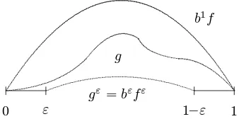
(d) (diffusion coefficient)g belongs to the set G0 _{of functions} _g_{: [0,}_1]_7−→_R+ _{(see Figure 1)} which are Lipschitz continuousand satisfy

g(0) = 0 =g(1) and g >0 on (0,1). (4)

(e) (drift parameters) The sequence {ck ≥0; k ≥ 1} of drift parameters with values in R+ satisfiesP_kck/N2k_<_∞.

3

Definition 1.2 (initial state) We often use a random initial stateX(0).Then X(0) is assumed to beindependent of the system w of driving Brownian motions. The lawL X(0) is denoted by µ. In most cases we assume thatµ belongs to the set Tθ of all those distributions on [0,1]Ξwhich areshift ergodic withdensityθ∈(0,1), that isRµ(dx)xξ ≡θ. WriteIPµ:=IPµg for the distribution ofX ifµis the initial law L X(0), andIPz:=IPzg in the degenerate caseµ=δz, z∈[0,1]Ξ. 3

Example 1.3 (interacting Fisher-Wright) The standard example is theinteracting Fisher-Wright diffusion with diffusion parameterbwhere by definition

g(r) :=bf(r) with f(r) :=r(1−r) and b >0; (5) see Figure 1. By an abuse of notation, in this case we also writeIPb

µ andIPzb for the laws ofX. 3

Example 1.4 (Ohta-Kimura) Another important case in genetics is theinteracting Ohta-Kimura dif-fusionwhereg=bf2

(5)

g∈ G0

0 1 0 1

[image:5.612.222.385.107.150.2]

f

Figure 1: Diffusion coefficients: Generalg and standard Fisher-Wrightf

Remark 1.5 (hierarchical groupΞ) We recall the followinginterpretationof Ξ used in mathematical biology: ξ= [ξ1, ξ2, ...]labels theξ1-st member in a family, which is theξ2-nd family of a clan, ..., which is

theξk-th member of ak–level set.kξ−ζk=krefers torelativesξ, ζ of degreek.

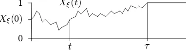
The system (1) occurs as diffusion limit of genetics models with resampling and migration (Moran model). ThenXξcan be interpreted as agene frequencyof theξ-th component (colony) of the system. (See Sawyer and Felsenstein [SF83] or Chapter 10 in Ethier and Kurtz [EK86].) 3 The basic features of the model stem from a competitionbetween drift and noise. Namely, set for the momentck ≡0, then all componentsXξfluctuateindependentlyaccording todiffusions with coefficientg. For instance in the Fisher-Wright case (5),Xξ will be trapped at 0 or 1 in finite time, as indicated in Figure 2.

0 Xξ(0) 1

t Xξ(t)

τ

Figure 2: Underck ≡0: A single Fisher-Wright diffusion path trapped at 1

On the other hand, if we set g = 0, then X solves an infinite system of ordinary differential equations, which has the property that, under ck >0, for initial states in Tθ (Definition 1.2) the solutionXt converges ast→ ∞ to theconstant stateθthat isθξ ≡θ.

Therefore in the case ck 6 ≡0, g 6= 0, the drift term is in competition with the basic feature of the diffusion of the single components to get trapped at{0,1}and in fact prevents it from getting trapped at all in finite time (except ifX starts already with either of the traps 0 or 1).

In the sequel we shall study only the case whereck ≡a >0, which is the prototype displaying a specific “critical” behavior. Namely, this special choice of the drift parameter implies first of all that we are in the regime ofclustering(for whichP_kc−_k1=∞would suffice), that is

IPXξ(t)−Xζ(t)≥ε −−→

t→∞0, ξ, ζ∈Ξ, ε >0. (6)

[image:5.612.210.401.326.378.2]

(6)

for generalck, see Dawson and Greven [DG93] (concerning the mean field limit) and Klenke [Kle95]. Much of the scheme we derive to study the cluster-formation in time can be performed as well for the label setZZ2.

1.2

Transformed Fisher-Wright tree

In order to discuss clustering phenomena, we want to introduce some objects which shall play a basic role in the description of the genealogy of clusters in this type of interacting models, as the backward tree in spatial branching theory does. Start with the following basic ingredients.

Definition 1.6 (Fisher-Wright) Fixθ∈(0,1).

(a) (standard Fisher-Wright diffusionYθ₎ _Let_B _{denote a standard Brownian motion, and} Yθ₌_Yθ_{(t); 0}_≤_t_{≤ ∞} _{the strong solution of}

dYθ(t) =

q

Yθ_(t)₁₋_Yθ_(t)_dB(t), ₀_{< t <}_∞, _Yθ_{(0) =}_θ. ₍₇₎

(b) (fluctuation times)We call the hitting time

τ := infnt >0; Yθ(t)∈ {0,1}o∈(0,∞) (8)

of the traps thefluctuation timeofYθ _{(cf. Figure 2 above).} (c ) (transformed Fisher-Wright diffusionYfθ₎_Set

f

Yθ_{(β) :=}_Yθ _log(1/β)_, ₀_≤_β_≤_1, ₍₉₎

and denote themarginal lawsof this time-inhomogeneous Markov process by

f

Qθ

β:=L Yfθ(β)

, 0≤β≤1. (10)

(d) (holding time of Yfθ₎_{Introduce the}_{holding time}_of _Yfθ_:

e

τ:= e−τ ∈(0,1). 3

Consequently, a path of the transformed Fisher-Wright diffusionYfθ_{starts at 0 or 1, namely with} the law ofYθ_{(τ), that is with}

(1−θ)δ0+θδ1, (11)

stays there for the random timeτe∈(0,1). Afterτ, the path fluctuates like a standard Fisher-Wrighte

diffusion but with time reversed and on a logarithmic scale, and finally ends up at timeβ = 1 at the deterministic valueθ. (Read Figure 2 backwards.) Note that (9) can alternatively be written asYfθ_(e−t_{) =}_Yθ_(t), ₀_≤_t_{≤ ∞.}

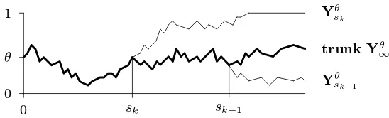
Next we compose a whole tree of Fisher-Wright diffusions (see Figure 3):

Definition 1.7 (Fisher-Wright tree Yθ₎ _Fix _θ_∈_(0,₁₎_, _k_≥_{1, and (deterministic) time points} 0≤sk<· · ·< s1< s0:=∞.

(a) (trunk)First we introduce thetrunkof the tree denoted byYθ

(7)

0 θ

1 Yθ

sk

trunk Yθ ∞

Yθ sk−1

sk sk−1

[image:7.612.166.440.97.180.2]

0

Figure 3: Fisher-Wright tree (only one branch trapped so far)

(b) (branches) Next we define the branches of the tree. Given the trunk Yθ

∞, let a branch Yθ

sk split away from the trunk at the timesk. The branch is again assumed to be standard

Fisher-Wright, but defined on the time interval [sk,∞], that is starting at time sk with Yθ

sk(sk) =Y

θ

∞(sk). Proceed with the other si accordingly. The branchesYsθi leaveonlyfrom

the trunk Yθ

∞ and are constructed independently of each other, given the trunk. Hence, by definition all the branches Yθ

si, k ≥ i ≥ 1, are conditionally independent given Y

θ

∞. Note that all the finitely many branches and the trunk end up in the set{0,1}of traps after finite times.

(c ) (fluctuation time of the trunk)As in Definition 1.6 (b), denote byτ thefluctuation time

of the trunk. Of course, given Yθ∞(τ) =∂ ∈{0,1}, all branchesYθsi with si ≥τ are trapped

at∂.

(d) (law and filtration)For the fixedsk, ..., s1, writePθ _{for the law of the Fisher-Wright tree} Yθ _and _{F_(t); _t _≥_0}_{for the related filtration (with} _{F(t) describing the behavior of} _Yθ _in

[0, t]). 3

Remark 1.8 The somewhat unexpected index∞=s0 (instead of 0 orsk+1) on the symbolYθ∞ for the

trunk of the tree will become clear below when we switch to a transformed tree. This also indicates that one could read the trunk in backward direction while then the branches, starting withYθ

s₁, split off in time viewed forward. This is (for good reason) the same as with the backward tree in branching theory, see for instance Chapter 12 in Dawson [Daw93]. – Note also that for typographical simplification we do not display

the time pointssk, ..., s1 in the notation of Yθ orPθ. 3

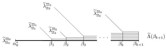
In analogy with the transformed Fisher-Wright diffusionYfθ _{defined in (9), we will introduce a} transformed Fisher-Wright tree Yfθ_{, see Figure 4, by starting from the Fisher-Wright tree} _Yθ _of Definition 1.7 and switching to the time scale e−s_=:_β _∈_[0,_1]. _{(Read the flat parts in Figure 4 as} being exactly at the boundaries.)

1 θ

0 1 β3

β2 β1

0

f

Yθ β3 f

Yθ β2

trunkYfθ 0

f

Yθ_β

1

e

τ

Figure 4: Transformed Fisher-Wright tree

(8)

(a) (trunk)Thetrunkof the transformed Fisher-Wright tree is

f

Yθ

0:=Yθ∞ log(1/·)

=Yθ _log(1/·)₌_Yfθ_.

(b) (branches)Thebranches Yfθ

β1, ...,Yfθβk are defined by

f

Yθ

βi(α) :=Y

θ

log(1/βi) log(1/α)

, 0≤α≤βi, 1≤i≤k. (12) Since α = 0 is included, the trunk and all branches start from the traps {0,1} and stay there for a positive time. The branchYfθ

βi terminates at the (deterministic) timeβi when it

coalesces with the trunk; henceYfθ_β

i(βi) =Yfθ0(βi). Consequently,Yfθcan be considered as a

coalescing ensemble of transformed Fisher-Wright diffusions. Note that by Definition 1.7 (b), all the branchesYfθ_β

i, 1≤i≤k,areconditionally independent givenYfθ0.

(c ) (holding time of the trunk)As in Definition 1.6 (d), denote byτe theholding time of the trunkYfθ

0. Note that

f

Yθ

βi(α) =Yfθ0(α) if 0≤α≤βi≤eτ, (13)

i.e. branches with terminal time bounded byτeare trapped at the trunk.

(d) (filtration)SetF(β) :=e F log(1/β), 0≤β≤1,(withF(β) describing the behavior ofe Yfθ

in [β,1]). 3

Remark 1.10 (Trees of transformed diffusions) Trees of transformed diffusions turned out to be a basic object entering into the description of cluster-formation of interacting diffusions. This applies for instance to interactingcritical Ornstein-Uhlenbeck diffusions,that is g(r) =σ2 >0, r ∈R, where one has a tree of Brownian motions, and tosuper-random walks, that is g(r) = σ2_{r, r} _≥_0, _{which lead to a} tree of more complicated but explicitly known time-inhomogeneous diffusions. 3

1.3

Time structure of components

Expected phenomena We start by discussing the phenomena to be described. The formal set-up and related results will be contained in the next two subsections.

For the remainder of the introduction we require:

Assumption 1.11 (initial state) Xstarts off with a shift ergodic distributionµwith fixed density

θ∈(0,1), that isµ∈ Tθ. 3

Thebasic theoremfor the interacting diffusion in the regime of clustering is

L X(t)===⇒

t→∞ (1−θ)δ0+θδ1, for L X(0)

=µ∈ Tθ, (14)

(where the symbol =⇒refers to weak convergence); see Cox and Greven [CG94].

Nevertheless, if we fix a label ξ in the hierarchical group Ξ, we proved in [FG94, Theorem 5] that for the correspondingcomponent process {Xξ(t);t≥0} in [0,1],

lim sup

(9)

time close to the traps{0,1}, [FG94, Theorem 4]. (Note that the oscillation property (15) can be interpreted as a type of“recurrence” property for clusters.)

We now want to know more about the durations for whichXξ is close to 1 or close to 0 (life times of clusters, or alternatively about correlation length in the time of our system). This should be closely related to the spatial cluster-formation.

We studied the cluster extensions in space in [FG94, Theorem 3]: At timeNβt_(as _t_{→ ∞), the} spatial clusters are of “size”αt, whereαis arandomelement of the open interval (0, β) (withβ >0 fixed which could be set to 1 by scaling). More precisely, we haveα=βeτ withτethe holding time of the transformed Fisher-Wright diffusion (Definition 1.6 (d)).

Or from another point of view, at time scaleNβt_{correlations in space are built within distances} of orderαt, with the same randomα. Or turned around, clusters of a spatial extension over a ball of radiusαt need at least time N(α+ε)t _{to be formed with positive probability, for some} _{ε >} _0. Combined with (15) this means that smaller clusters keep being overturned or melted with other smaller ones. This suggests that in order to describe the sequence ofholding timesof values close to 1 or close to 0 on a large scale, we should encounter four interesting phenomena. Namely the holding times should be

– of a random order of magnitude,

– asymptoticallysmall compared with the age of the system and

– (stochastically)monotoneand of increasing order of magnitude, within the correlation length, – comparable with the correlation length.

To see that the correlation length is of a smaller order than the system age, look (for the fixed ξ) at{Xξ(βt); 0< β≤1}. The law of this process converges ast→ ∞to a“stationary”0-1–valued

noise; see Proposition 6.1 at p. 39. (Compare this phenomenon of a noisy behavior in time with the occurrence of a spatial “isolated Poissonian noise” in the analysis of the clumping in the time-space picture for branching systems in low dimensions [DF88].)

To elaborate on this point look at the exponential scale Nβt _{and at a} _{component process}

Xξ(Nβt_{); 0}_{< β}_≤₁ _{(for the fixed} _{ξ). As} _t _{→ ∞} _{we get the same limiting “stationary” 0-1–} noise. That is, the limit is independent in each “macroscopic” time point β, where the common one-dimensional marginal is just (11), withθ ∈(0,1) the initial density of the system. The latter fact follows from (14).

This indicates that in order to capture time correlations we have to study Xξ after very long times but on a much finer scale thanβ as it appears in Nβt_{. To accomplish that, we will look}

backwards from late time points NT _{in time scales of smaller order. This will be incorporated} formally by the following set-up.

Results To capture the structure of the correlations in time of the component process, we will look at an asymptotically small neighborhood of a late time point. For fixedξ∈Ξ and T >0, we define thescaled component process,

U_βT :=Xξ NT −NβT, 0≤β <1, (16)

that isβ ∈[0,1) becomes the “macroscopic backward time”. Consequently, from the “terminal time” NT we lookbackwards for the amountNβT whereβ varies in [0,1). Note thatNT−NβT ∼NT as T→ ∞, so that the whole process UT indeed describes the behavior “close to”NT.

Recall that g ∈ G0 _and _µ _{∈ T}

(10)

Theorem 1 (scaled component process) Fix a label ξ∈Ξ.

(a) (convergence) There is a {0,1}–valued process U∞ _{on the (macroscopic backward) time}

interval[0,1)such that

UT ₌fdd₌_⇒_U∞ _as _T _{→ ∞.} (b) (characterization of U∞₎_For_k_≥₀_and ₀_≤_β

0< β1< ... < βk<1:

IPnU∞

β0 =...=U

∞ βk = 1

o

= EYfθ_(β

0)· · ·Yfθ(βk)

= E Yfθ_(β k)k+1.

Consequently, the distribution of U∞ _{is a mixture of Bernoulli product laws: First realize the}

transformed Fisher-Wright diffusionYfθ _{and then build the product law with marginals}

1−Yfθ_(β)_δ0₊_Yfθ_(β)_δ1_, ₀_≤_{β <}_1. ₍₁₇₎

In particular, the one-dimensional marginals L U∞ β

are given by(11), for all β ∈[0,1).

(c ) (qualitative description of U∞₎ _{Consider the holding time} hU := supβ∈[0,1);Uβ∞=U0∞ ∈(0,1)

of the initial stateU0∞. Then

L [U₀∞, hU]

=L fYθ_(0),_e_τ_.

Furthermore, beyond hU the process U∞ is a “mixture” of non-stationary 0-1–noise: For

∂∈ {0,1}and theβ1, ..., βk as in(b),

LhU_β∞₁, ..., U_β∞_ki U₀∞=∂, hU < β1

= E

_Q

k i=1

h

1−Yfθ_(β i)

δ0+Yfθ(βi)δ1

i

Yfθ(0) =∂, eτ < β1

.

Remark 1.12 Note that the holding timehUismeasurableon theσ–algebra of all (backward) paths with

a non-empty starting interval of constant value. 3

The theorem says three things:

(i) If we look back from timeNT _{in time scale}_NβT_{, the component we focus on has been “close”} to its state∂ for a time of random orderβ of magnitude.

(ii) This order is (strictly) positive and coincides in law with the holding timeτeof Yfθ_.

(iii) Later changes occur in times of a smaller order of magnitude (conditional noise), within the correlation length.

Remark 1.13 (time average of components) Since the correlation length (in time) is small com-pared with the system’s age, one could prove that objects of the formt−1Rt

0 ds Xξ(s) converge in law to θ. This is characteristic for the case of drift parameters{ck}not decaying exponentially fast (the analog of

(11)

0 ε 1−ε 1

r r

HT

2 H1T

[image:11.612.174.430.100.189.2]

NT

Figure 5: Alternating sequence of “holding times”

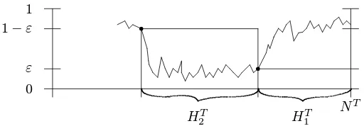
An open problem A very natural question is, how the holding times close to time points NT behave in the limitT → ∞. To be a bit more specific, for a fixedε∈(0,1

2) we introduce a sequence of random (backward) times (see Figure 5):

n

NT−P₁_≤_i_≤_nH_iT; n≥1o.

HereHT

1 is by definition the (first) hitting (backward) time of the boundary [0, ε] if we start off at timeNT _{in [1}₋_ε,_{1], or vice versa.} _HT

2 is then defined as the hitting (backward) time increment of the opposite boundary region starting at timeNT−H₁T, etc. At this stage we agree to set a hitting time incrementHT

i (together with the subsequentHjT, j > i) equal to 0 if the time interval [0, NT] is exhausted.

For our purpose, the incrementsHT

1, H2T, ...may serve as the (backward) holding times of the component processXξ at the boundaries, since the fraction of time the component process spends in [ε,1−ε] converges to 0 in probability asT → ∞; see Theorem 4 in [FG94].

Incorporating the scaling suggested by the result of Theorem 1, define therescaled holding times

b

H_iT := logH T i

TlogN (18)

(that is NHbT

iT = HT

i ) which for our purpose describe the order of magnitude of HiT. What one would like to do now is the following:

– Show thatL bHT

i ;i≥1 has a limiting law, say Γ. – Identify the law Γ via the transformed Fisher-Wright tree. – Show that Γ is concentrated on decreasing sequences.

In order to carry out such an analysis, which involves joint laws of holding times rescaled by functions of different order of magnitude, requires more than controlling moments of the time-space diagram. What is needed is a representation of the interacting system via particle systems in the sense of the work of Donelly and Kurtz [DK96]. Such analysis is outside the scope of the present paper.

1.4

Spatial ball averages in time dependence

(12)

For fixedξ∈Ξ andα∈[0,1) consider the followingspatial ball averages

V_βα,T := 1 N[αT]

X

ζ:kζ−ξk≤αT

Xζ NT−NβT= Xξ,[αT] NT −NβT

, (19)

0≤β <1, as processes in themacroscopic backward timeβ ∈[0,1) (here [r] refers to the integer part ofr). AsT → ∞, a limiting process Vα,∞ _{on [0,}_{1) will exist whose law depends on}_{α. Since} NβT ₌_o(NT_{) (for}_{β <}_{1 fixed), we stay again within the correlation length, and the one-dimensional} marginal distribution of Vα,∞ _{is again independent of} _β _{but is now given by the law}_Qfθ

α of the transformed Fisher-Wright diffusionYfθ _{of (9) at}_α_{; see [FG94, Theorem 2].}

The next theorem deals with this time-scaled process of spatial ball averages. Recall thatµ∈ Tθ and 0< θ <1.

Theorem 2 (time-scaled spatial ball averages)Fix0≤α <1.

(a) (convergence)There exists a [0,1]–valued processV_βα,∞; 0≤β <1 with

Vα,T =fdd=⇒Vα,∞ as T → ∞. (20)

(b) (characterization of Vα,∞₎ _Fix_{k, m0}_{, ..., mk}_≥₀_and _{0 =:}_β0_<_{· · ·}_{< βk}_<₁_{. Then} IE V_βα,∞

0 m0

··· V_βα,_k∞mk

= EθYfθ 0(α)

m0+···+mJ−1 Y

J≤i≤k

f

Yθ βi(α)

mi

with Yfθ _{the transformed Fisher-Wright tree of Definition} _1.9_{, and}

J := mini; α≤βi, 1≤i≤k+ 1 . (21)

(c ) (qualitative description of Vα,∞₎

(c1) The marginal laws L V_βα,∞are given by Qfθ

α of Definition1.6 (c), for all β∈[0,1). (c2) Consider hV := sup

β ∈ [0,1); V_βα,∞ = V₀α,∞ , the holding time of Vα,∞ ₍_recall

Remark1.12). ThenL(hV) =L(α∨eτ) (see Definition 1.6 (d)).

(c3) Beyond hV the finite-dimensional distributions of Vα,∞ are equal to LhV_βα,₁∞,...,V_βα,_k∞ihV< β1

=LhYfθ_β

1(α),...,Yfθβk(α)

i

(α∨eτ)< β1

(with theβi from (b)). Here the r.h.s. is the following mixture of product laws:

Z

Rθ,α_β

1,...βk d

θ1, ..., θk gQθ1

α/β1× · · · ×Qg

θk

α/βk,

withRθ,α_β

1,...βkthe conditional distribution of

h f

Yθ_(β

1),...,Yfθ(βk)

i

given(α∨eτ)< β1, and

withQgθi

(13)

This theorem says that the spatial ball average has remained in its terminal value at least a time of orderNαT_{. However, this holding time is larger than}_α_{if the whole}_{α–ball is covered by a 0– or} 1–cluster at the terminal timeNT _{(this event has positive probability), in which case (depending on} the random size of that cluster) the empirical mean had been in the same state as at timeNT _for a random time. The order of magnitude isα∨eτ. Looking back further gives us then conditionally (givenα∨eτ) independent observations since the time grid is too large to detect earlier and hence small holding times. Theorem 2 (c) combined with the conjectures at p. 11 and a result in [FG94] suggests that a specific value in the order of magnitude of the holding time of a component (viewed backwards from a late time point) corresponds to the existence of a cluster at that late time which has acorresponding order of magnitude. Roughly speaking, on the used macroscopic scales, the spatial cluster size gives the holding time of a typical component in that cluster. This will be made precise in Theorem 3 below.

1.5

Time-space thinned-out systems

A second approach to investigate the history of a spatial cluster found at timeNT _{and to relate the} order of spatial size of the cluster to the order of the holding time of a component, is the following. Choose a spatial network of points having distancesαT. Consider a new field obtained by observing the system through time only at this network of observation points. Do this however only in a network of time points which also spread apart suitably as the system ages. We formalize this point of view as follows which will verbally be explained in Remark 1.15.

Definition 1.14 (thinning procedures) (a) (inverse level shift operatorsS−1

n and spatially thinned-out systemsSn−1x)Forn≥0, ξ∈Ξ andx∈[0,1]Ξ_{, set}

(S_n−1x)ξ :=xS−1

n ξ with (S

−1 n ξ)j :=

(

ξn+j if j > n,

0 if 1≤j≤n. (22)

(b) (space-time thinned-out systems)Fixk≥0 and 1> β1>· · · > βk ≥α >0 =:β0. Set β:= [β1, ..., βk] and

W_ξ,iβ,α,T := S_[αT−1_]X_ξhNT− X 1≤i′_≤_i

Nβi′T

+

i

, (23)

ξ∈Ξ, 0≤i≤k, T >1. 3

Remark 1.15 S−1

n shifts all coordinates (levels) of ξbynsteps, and fills in the newly created coordinates by 0. Hence,ξ= 0 is a fixed point, and ifkξk=m6= 0 thenkS−1

n ξk=m+n. In particular,S−

1

n increases non-zero distances of pairs of labels byn. Applied to a whole configuration x∈[0,1]Ξ

, we can viewS−1

n x as aspatially thinned-out systemsince each fixed pair of labels has distancen.

For the fixed scaling parametersβ ≥α, we consider [ξ, i]∈Ξ× {0, ..., k}as new, macroscopic space-“time” variables of the random fieldsWβ,α,T

. AsT → ∞, these fields will have a{0,1}Ξ×{0,...,k}

–valued limiting field denoted byWβ ,α,∞_{. It describes the evolution of clusters both in time and space.}

3

Theorem 3 (time-rescaled thinned-out systems)Fix scaling parametersβ ≥αas in Defini-tion1.14 (b).

(a) (convergence)There exists a {0,1}Ξ×{0,...,k}_{–valued random field} _Wβ,α,T _on _Ξ_{× {0, ..., k}}

such that

(14)

(b) (characterization of Wβ,α,∞) Fix natural numbers m0, ..., mk ≥ 0 and, for each i in

{0, ..., k}, distinct labelsξi,1, ..., ξi,mi in Ξ. Then

IP

W_ξβ,α,_i,j_,i∞= 1; 0≤i≤k, 1≤j≤mi= EθQk_i=0 Yfθ_β

i(α)

mi

(24)

withYfθ _{the transformed Fisher-Wright tree of Definition}_1.9 _(and_β 0= 0).

(c ) (qualitative description of Wβ,α,∞) W_ξ,iβ,α,∞; ξ ∈ Ξ, 0 ≤ i ≤ k is an associated collection of {0,1}–valued random variables. To describe its distribution, letFβ,αdenote the law of the random vector fYθ

βi(α); 0≤i≤k , and write ∂ for the configuration identically

equal to∂. Then

L Wβ,α,∞ =

Z

Fβ,α du0, ..., ukh Qki=0(1−ui)δ0+uiδ1

iΞ

= P_∂=0,1 PYθ_(τ_{) =}_{∂, τ} _≤_log(1/β 1)

δ∂

+Eθ

Qk

i=0

h

1−Yfθ_β

i(α)

δ0+Yfθ_β

i(α)δ1

iΞ

; eτ < β1

.

Consequently, Wβ,α,∞ is a “mixture” of independent fields; with probability P(τe≥β1)it is

even a constant field∂ (with random∂).

Theorems 1 (c) and 3 (c) reflect the fact that clusters have a space-time extension with an order of magnitude (α, α) where αis random. That is, the spatial cluster size isαT (in the hierarchical distance), whereas a “typical” component of that cluster lived for a timeNαT_{. Or turned around,} at timeNT_{, spatial clusters of size}_αT _{have an age of order}_NαT_{. Hence, in the time-space diagram} of the process viewed back from the end NT _{in an exponential time scale, we see at large times} clusters of a size comparable with a square of a random size.

Remark 1.16 Both marginals of the fields are mixtures of product laws, and the mixing distributions are

expressed via Fisher-Wright tree quantities. 3

The most important feature of our analysis is that the large scale behavior of our model does not depend on the diffusion coefficientg, and in particular the transformed Fisher-Wright tree is an

universal objectin the class of models considered:

Corollary 1.17 (universality) The limiting objectsU, V, and (in the sense of finite-dimensional distributions)W depend essentially on the initial density θ∈(0,1), but are otherwise independent of the “input parameters” a > 0, g ∈ G0 _and _µ _{∈ T}

θ of the interacting diffusion X, and of the

parameter N of the label set Ξ.

1.6

Strategy of proofs and outline

(15)

For this purpose, in Section 2 we study some random walk systems, in particular coalescing random walks. In Section 3 we introduce an extension of Kingman’s coalescent. We call this object

e

Λ an ensemble of log-coalescents. In Section 4 it occurs in certain scaling limits of coalescing random walks (e.g., Theorem 4 at p. 27). On the other hand, it is in duality with the transformed Fisher-Wright treeYfθ _{(Theorem 5 in Section 4, p. 31), which is our crucial object for the description of the} space-time structure of interacting diffusions. In Section 5 other basic techniques like the duality of X andϑ, coupling and moment comparison are compiled, culminating in the universal conclusion Theorem 6 at p. 37. In Section 6 we finally prove our Theorems 1–3 and with Theorem 7 (p. 39) a rather general version of a scaling limit for thinned-outX–systems.

2

Preliminaries: On coalescing random walks

A basic tool for our study of the interacting Fisher-Wright diffusion X will be a time-space duality relation with a delayed coalescing random walk with immigration. As a preparation for this, in the present section we develop the relevant random walk models and some of their properties.

2.1

Coalescing random walk with immigration

Random walk Z on the hierarchical group Ξ Let Z = {Zt;t≥0} denote the continuous-time (right-continuous)random walk in Ξ withjump rate

κ:= aN 2

N2₋₁ (25)

(whereais the drift parametera≡ckof the interacting diffusion of Definition 1.1 andNthe “degree of freedom” in the hierarchical group Ξ) andjump probabilities

pξ,ζ:= 1

N2kζ−ξk, ξ6=ζ, hence pξ,ξ≡ N−1

N . (26) LetZξ _{refer to}_Z_{starting with}_Z_{(0) =}_ξ_∈_{Ξ (at time 0). The law of} _Z₌_Zξ _{is denoted by}_Pξ_{. For} convenience sometimes we also writeZ(t) instead of Zt (similarly we proceed for other processes). We recall from [FG94, Lemma 2.21 and Proposition 2.37] thatZis arecurrentrandom walk and that the hitting timedistribution of the origin starting from a fixed point ξ6= 0 has tails of order 1/logt ast→ ∞. For a detailed study of this random walk we refer to Section 2 of [FG94]. Delayed coalescing random walk ϑ Letϑ={ϑξ(t);ξ∈Ξ, t≥0}denote the (right-continuous)

delayed coalescing random walk in Ξ withcoalescing rateb >0 (which corresponds to the diffusion parameter of the interacting Fisher-Wright diffusion, recall (5)). By definition, in the delayed coalescing random walkϑthe particles move according to independent random walks of the previous subsectionexceptwhen two particles meet. In the case of such a collision, as long as the two particles are at the same site, they attempt to coalesce to a single particle with (exponential) rateb.

Writeϑψ _if_ϑ_{starts (at time 0) with}_ψ_∈_{Ψ. Here Ψ}_⊂_ZZΞ

+ denotes the set of all those particle configurationsψ={ψξ;ξ ∈Ξ}which are finite: kψk:=Pξψξ <∞. The configurationsψ with kψk= 1 (unit configurations) are denoted byδξ _where _ξ_∈_{Ξ is the position of the particle. Set}

(16)

For a detailed description and discussion of ϑwe refer to §3.a in [FG94] where the model is called coalescing random walk with delay. (ϑ is the dual of the interacting Fisher-Wright diffusion, see (64) at p. 34 below.)

Coalescing random walk η Write η = ηϕ_{, ϕ} _∈ _{Φ, for the (instantaneous)} _{coalescing random}

walk obtained by formally setting the coalescing rate b to∞.Here Φ denotes the set of all (finite) populationsϕ ∈ Ψ with at most one particle at each site, that is ϕξ ≤ 1 for all ξ; see §3.c in [FG94] for a detailed exposition. (Recall thatη is the dual of the voter model on Ξ with interaction described byκ pξ,ζ of (25) and (26); see Liggett [Lig85, Chapter 5].)

By an abuse of notation (no confusion will be possible), the distributions of ηϕ _and _ϑψ _are written asPϕ _and_Pψ_{, respectively.}

Delayed coalescing random walk with immigration As introduced above, the delayed ran-dom walkϑψ _{starts at time} _t

0 = 0 with ϑ(0) = ψ. Now we modify the model in the following way. Consider a finite sequencet0, ..., tk∈IRof (deterministic) time points and related (determinis-tic) populationsψ0_{, ..., ψ}k_∈_{Ψ, respectively. Start the delayed random walk at time}_t∗ _:=_t

0∧...∧tk with the related populationψ∗_{, but in addition let the related populations}_ψi _immigrate _{at the} remaining time pointsti 6=t∗, i= 0, ..., k.The resulting (right-continuous) delayed coalescing

ran-dom walk with (deterministic)immigrationis again denoted byϑ but we exhibit the immigration parameters in the notation as follows:

ϑ=ϑψ_t₀0_,...,t,...,ψ_kk, P_tψ₀0_,...,t,...,ψ_kk, t0, ..., tk∈IR, ψ0, ..., ψk∈Ψ.

In particular, the starting time point is also viewed as an immigration time point. Of course, in the casek= 0 andt0= 0 we are back to the original delayed coalescing random walk: P0ψ=Pψ.

Note that this family of (time-inhomogeneous) Markov processes has an obvious generalized time-homogeneity property:

Pψ_t₀0_,...,t,...,ψ_kknϑtk+t∈ ·

ϑtk−=ψ

′o₌ _Pψ′_+ψk

{ϑt∈ ·}, (28)

t0, ..., tk−1≤tk, t≥0, ψ0, ..., ψk, ψ′ ∈Ψ.

Coalescing random walk with immigration Similarly we defineη, the (instantaneous) coalesc-ing random walk with immigration(whereb=∞) and use the notation

η =ηϕ_t₀0_,...,t,...,ϕ_kk, Pϕ_t₀0_,...,t,...,ϕ_kk, t0, ..., tk∈IR, ϕ0, ..., ϕk∈Φ.

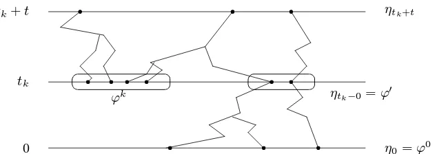
These processes have a generalized time-homogeneity property analogous to (28). In this case one should have in mind a picture as shown in Figure 6.

The delayed coalescing random walk process with immigration is in a time-space duality with the interacting Fisher-Wright diffusion process, see Proposition 5.1 at p. 34, whereas the (instantaneous) coalescing random walk with immigration is in a time-space duality with the voter model on Ξ. The word time-space refers here to the fact that we consider the whole path up to timet. (In the case of Ξ =ZZd with interaction determined by the simple random walk kernel pξ,ζ, the latter time-space duality was developed in Cox and Griffeath [CG83] using the name “frozen” random walks instead of ones with “immigration”.)

2.2

Basic coupling

Throughout the paper it will be useful to define the relevant random walk models on a common

(17)

tk+t

tk

0 η0=ϕ0

ηtk+t

ηtk−0=ϕ′

ϕk

r r r

pr r r r r r

[image:17.612.150.467.101.213.2]

r r r

Figure 6: Coalescing random walk with immigration (0 =t0< tk < tk+t, k= 1)

walks with immigrating populationsχ0_{, ..., χ}k _∈ _{Ψ at the times} _t

0, ..., tk, respectively, defined as Ψ-valued process in the obvious way. Finally we give the followingbasic coupling principle:

Construction 2.1 (basic coupling)Choose a basic probability space[Ω,F,P]in such a way that it supports all three (time-inhomogeneous) Markov families

Z_tχ₀0_,...,t,...,χ_kk, ϑ_tψ₀0_,...,t,...,ψ_kk, and ηϕ_t₀0_,...,t,...,ϕ_kk,

where k≥0, t0, ..., tk∈IR, χ0_{, ..., χ}k_{, ψ}0_{, ..., ψ}k _∈_Ψ _and _ϕ0_{, ..., ϕ}k _∈_Φ_{, and that these families}

satisfy

Z_tχ₀0_,...,t,...,χ_kk(t) ≥ ϑψ_t₀0_,...,t,...,ψ_kk(t) ≥ η_tϕ₀_,...,t0,...,ϕ_kk(t), t≥t∗:=t0∧...∧tk,

whenever χi_≥_ψi_≥_ϕi _{for all} ₀_≤_i_≤_k_.

Proof (existence of the basic coupling) First construct a probability space which supports the family ofindependent random walks with immigrationZ_tχ₀0_,...,t,...,χ_kk. Then at timet∗ we startkχ∗k independent walks placed according to the relatedχ∗_{, at all the remaining times}_ti _{we additionally} startkχi_k _{independent walks placed according to} _χi_{. But in addition every immigrating particle} (including at timet∗_{) gets an internal degree of freedom, by definition one of the numbers 0,}_{1 or 2.} The rules are as follows: If the immigrating particle belongs to one of theϕi _{it gets the 0-mark, in} the case of particles fromψi₋_ϕi _{we adjoin the mark 1, and for} _χi₋_ψi _{we take 2. The mark of a} particle is preserved during its evolution except for the following two situations:

• If two particles meet which have both the mark 0, then one of them (chosen at random) instantaneously gets the mark 1.

• If a pair of particles with mark in{0,1}(except if both are 0) stays at the same site, then at exponential rate bone of them having mark 1 is chosen at random (if we have two of them) and increases it’s mark from 1 to 2. Here we let all possible pairs (at the same site) act independently.

Then at timet≥t∗_{count the particles as follows:}

b

Z_tχ₀0_,...,t,...,χ_kk(t) := particles of all marks

b

ϑψ_t₀0_,...,t,...,ψ_kk(t) := particles with marks 0 or 1

b

(18)

Apparently these processes satisfy Z(t)b ≥ ϑ(t)b ≥ η(t),b t ≥ t∗_, _{and are a version of} _{Z, ϑ, η} _as

wanted. 2

Note that the trivariate process [Z, ϑ, η] isnot Markov. (In defining bZ,ϑ,b bη by deleting the internal marks, the Markov character is lost.)

2.3

Approximation by (instantaneously) coalescing walks

Doubtless, (instantaneous) coalescing random walks with immigration are easier to handle than the corresponding delayed ones. On the other hand, we want to show now that in our context of a recurrentZ asymptotically the delayed coalescing random walk with immigration can be replaced without loss of generality by the corresponding system with instantaneous coalescence, and we will widely use this later on. (This implies in particular that the clustering properties of interacting Fisher-Wright diffusions are independent of the diffusion parameterb >0.)

On anintuitive level this equivalence is justified by the following argument: If two particles do not meet, then the coalescing rateb is irrelevant and can be set to∞. On the other hand, once two particles meet and do not coalesce before one of them jumps away, then byrecurrence they will meet again and again until they will finally coalesce. (Caution: This heuristic argument has to be refined since it does not take into account that one of these two particles could meanwhile be “absorbed” by another particle.)

To put this idea on a firm base, first associate with eachψ∈Ψ the“truncated”elementψ∧1∈Φ defined by (ψ∧1)ξ :=ψξ∧1, ξ∈Ξ. The following result is a refinement and generalization of the approximation Proposition 3.6 of [FG94].

Proposition 2.2 (approximation of ϑ by η) Fix integers m0, ..., mk ≥ 1, k ≥ 0. For t >1,

consider populations

ψi=ψi(t)∈Ψ with ψi=mi, 1≤i≤k,

and time points

s0(t)<· · ·< sk(t)< sk+1(t) with sj(t)−si(t)−−→

t→∞ ∞ if j > i.

Then on our basic probability space[Ω,F,P] (recall Construction2.1), the event

ϑ_sψ₀0_,...,s,...,ψ_kk(sk+1) = η_sψ₀0_,...,s∧1,...,ψ_k k∧1(sk+1) (29)

hasP-probability converging to 1ast→ ∞. (Sometimes we do not display the t-dependence.)

Remark 2.3 The approximate equivalence of ϑand η explains via duality, why (in the recurrent case) interacting Fisher-Wright diffusions and the voter model on Ξ have a similar large scale behavior. 3

Proof The proof proceeds by induction overk, the number of immigration time points.

(19)

step, recall the coupling Construction 2.1 and assume that the statement is true for somem−1≥1. Write

Em:=nϑψ(Nt) =ηψ∧1(Nt)o for the event (29) (in the casek= 0). DefineEm

m−1 as Em except replacingψ byψ−δζ(m,t). For a fixedi < m, letCi,t(s) andMi,t(s) denote the events that the walksZζ(i,t)and Zζ(m,t)coalesce respectivelymeetby times.

Letσ(t) denote the first collision time of Zζ(i,t)_and _Zζ(m,t) _{after at least one of them jumped} away from its initial state. Recall that the difference of the independent walksZζ(i,t)_and_Zζ(m,t)_{is a} random walk of the same kind except twice the jump rate. Defineα(t) byα(t)t=kζ(i, t)−ζ(m, t)k. By the hitting probability Proposition 2.43 of [FG94], we have forγ∈(0,1) fixed,

PnNt−Nγt≤σ(t)< Nto−−→

t→∞ 0. (30) (In fact, apply this proposition twice, namely withβ(t)≡1 and̺(t)≡ −∞or̺(t)≡γ, respectively.)

Consider a subsequence t′ _{→ ∞}_{such that the limit} _{α(∞) := lim}

t′_→∞α(t′) exists in [0,∞]. If

α(∞)≥1 then by the same proposition we have Pnσ(t′₎_{< N}t′o

−−−→

t′_→∞ 0. (31)

In the opposite caseα(∞)<1, the latter probability has a positive limit, and (30) implies PnMi,t′ Nt

′

−Nγt′ Mi,t′(Nt ′

)o−−−→ t′_→∞ 1.

But then due torecurrenceof the random walk (cf. Lemma 2.21 in [FG94]) we conclude PnCi,t′ Nt

′

Mi,t′ Nt ′o

−−−→ t′_→∞ 1

and therefore

PnMi,t′ Nt ′

\Ci,t′ Nt ′o

−−−→

t′_→∞ 0. (32)

On the other hand, from (31) we know that (32) holds also underα(∞)≥1. Summarizing (32) is true whenevert=t′ _{→ ∞.}

Dropping in notation the time argumentNt_{, we use the decomposition}

E_mm₋₁=

E_mm₋₁∩ [ i<m

Mi,t

∪

E_mm₋₁∩ C [ i<m

Mi,t

(33)

(whereCA denotes the complement of the eventA). By the induction hypothesis,PEm

m−1 tends to 1 ast→ ∞, so the probability of the event on the r.h.s. of (33) tends to 1. By (32) we can replace in that eventS_i<mMi,t bySi<mCi,t to get still

P

Em m−1∩

[ i<m Ci,t ∪ Em m−1∩ C

[

i<m Mi,t

−−→ t→∞ 1.

This finishes the proof by induction onmsince the latter event impliesEm. Consequently the claim in the proposition holds in the casek= 0.

2◦(induction step) Using that the pair [ϑ, η] is a simple functional of a (bivariate) Markov process (see§2.2) and exploiting generalized time-homogeneity as in (28), the induction step is similar to the argument fork= 0 by considering the process starting with the configuration at the moment

(20)

2.4

Speed of spread of random walks

Our random walkZ in Ξ has the following property: At time scale Nt _{the speed of growth of the} normkZ(Nt_)k_of _Z(Nt_{) is of order 1 as}_t_{→ ∞. To formulate with Lemma 2.6 below a more precise} statement, forr, c≥0, set

ℓ(r) :=N∨log[r]

logN , (34)

and introduce the subsets

Ξ[r, c] :=nξ∈Ξ;kξk ≤[r] +c ℓ(r)o, Ξ[r, c] :=nξ∈Ξ;kξk −[r]≤c ℓ(r)o, (35)

of Ξ which consists of all labelsξ, up to a specific logarithmic error, of at most or exactly norm [r]. Note that the ring Ξ[r, c] is contained in the ball Ξ[r, c], which is non-decreasing inr,and that both are non-decreasing inc. These sets have the following simple property.

Lemma 2.4 (spread of sums) Fix constants α, β, c, d ≥ 0 with α < β. For t > 1 let ξ(t) in

Ξ[αt, c]and ζ(t)in Ξ[βt, d]be given. Then, for all t sufficiently large,

ξ(t) +ζ(t)∈Ξ[βt, d]. (36)

Remark 2.5 (cancellation) The assumptionα < βcannot be dropped. For instance, ifα=β= 1 and

c=d= 0 as well asξ(t) :=−ζ(t) then ξ(t) +ζ(t)≡0∈/Ξ[t,0]. 3

Proof From the definition (35) we conclude

kξ(t)k ≤[αt] +c ℓ(αt), kζ(t)k ≥[βt]−d ℓ(βt).

Thenα < β yieldskξ(t)k<kζ(t)kfor allt≥t0say. Hence, kξ(t) +ζ(t)k=kζ(t)kfor thesetby the definition of addition in Ξ. Consequently, (36) holds fort≥t0. 2

The announced speed property of our random walk now reads as follows. Note that we choose the initial stateξ(t) of the random walkZξ(t)_itself _t-dependent.

Lemma 2.6 (walk speed) Fix non-negative constants α, α′ _{and positive constants} _{β, ε, c}_{. For} t >1, let̺(t)∈− ∞, β−ε_t, ξ(t) ∈Ξ[αt, c], andζ(t)∈Ξ[α′_{t, c]} _{be given. In the case} _{α > β}_,

require even that ξ(t)and ξ(t) +ζ(t)both belong to Ξ[αt, c]. Then

Pnζ(t) +Zξ(t) Nβt−N̺(t)t∈ Ξ(α∨α′∨β)t ,2co−−→

t→∞ 1. (37) In particular, ifkZ(0)kist-dependent and has a speed of orderαthen the speed of kZξ(t)_(Nβt_)k is of orderα∨β ast→ ∞; that is, the time correction termN̺(t)t_{is negligible.}

Proof Without loss of generality, in (37) we may set ζ(t)≡0. In fact,ζ(t) +Zξ(t) _{coincides in} law withZξ(t)+ζ(t)_{, and}_ξ(t)_∈_{Ξ[αt, c], as well as}_ζ(t)_∈_Ξ[α′_{t, c] imply}_{ξ(t) +}_ζ(t)_∈_Ξ[(α_∨_α′_{)t, c],} so in the caseα≤β we can rename ξ(t), ζ(t) and α. Moreover, in the case α > β we additionally assumedξ(t), ξ(t) +ζ(t)∈Ξ[αt, c], so again it is justified to renameξ(t) andζ(t).

(21)

the walkZ0 _{starting at the origin 0 of Ξ. By the proved part of the lemma, we may assume that} Z0 _Nβt_−N̺(t)t_{belongs to Ξ[βt,}_{2c]. Then, by Lemma 2.4, for}_t_{sufficiently large,}_Z0 _Nβt_−N̺(t)t₊ ξ(t)∈Ξ[αt, c]. Hence, Zξ(t) _Nβt₋_N̺(t)t_∈_{Ξ[αt, c]}_⊆_Ξ[αt,_{2c] with probability converging to 1}

ast→ ∞. This finishes the proof. 2

Remark 2.7 (non-cancellation) In the case α ≤ β, the cancellation effect of Remark 2.5 cannot happen in the situation of Lemma 2.6, since there is negligible probability that the walk will meet a prescribed

point at a particular late time. 3

2.5

Speed of spread of coalescing random walks

The above speed property of families of single random walks (Lemma 2.6) has consequences for the coalescing random walk with immigration, since we are interested in the latter system at late times and for time-dependent initial and immigrating populations. To describe the situation we need some notation (which is verbally explained below):

Definition 2.8 (spreading multi-colonies) Fix integersℓ, m0, ..., mℓ≥0 and non-negative con-stantsα0, ..., αℓ, c. Writeα:= [α0, ...αℓ] and m:= [m0, ..., mℓ].For t >1, denote by Φt[α , m;c] the set of all those populationsϕ=ϕ(t)∈Φ which can be represented as ϕ=ϕ0₊_{· ·}_+ϕℓ _where theϕj ₌_ϕj_(t)_∈_{Φ, 0}_≤_j_≤_{ℓ, have the following properties (recall (35)):}

(a) kϕj_{(t)k ≡}_mj_.

(b) If δξ _≤_ϕj _then_ξ₌_{ξ(t) has to belong to Ξ[αjt , c].} (c ) If δξ₊_δζ _≤_ϕj _{then we must have}_ξ₋_ζ_∈ _Ξ[α

jt , c]. (d) If δξ _≤_ϕj _and_δζ _≤_ϕj′

wherej6=j′thenξ−ζ∈Ξ(αj∨αj′)t , c.

If in (b) the balls Ξ[αjt , c] are replaced by the smaller rings Ξ[αjt , c] then write Φt[α , m;c] in-stead of Φt[α , m;c]. (Note that Φt[α , m;c] ⊆ Φt[α , m;c].) Finally, write Φt[α ,≤m;c] and Φt[α ,≤m;c] if in (a) onlykϕj(t)k ≡nj ≤mj for somenj. 3

Consequently, a populationϕ∈Φt[α , m;c] orϕ∈Φt[α , m;c]

,for which we often prefer to use the term“multi-colony”,is a superposition of ℓ+ 1 subpopulationsϕ0_{, ..., ϕ}ℓ_{of size}_m0_{, ..., mℓ}_≥_0, respectively, with the following properties (up to specific logarithmic errors):

• Particles from thej-th subpopulation spread at (respectively at most at) speedαj (see (b)). • Pairs of particles from thej-th subpopulation spread with relative velocityαj (cf. (c)). • Mixed pairs of particles from [ϕj_{, ϕ}j′

] spread at relative speed αj∨αj′(see (d)).

Now we are in a position to formulate the main result of this subsection concerning the speed of spread of multi-colonies in the coalescing random walk with spreading immigrating populations. In simplified words it says the following: Suppose at timessi(t) :=Nβit, i≤k, we have an immigration by populations being a superposition consisting of ℓi+ 1 subpopulations of mi,0, ..., mi,ℓi particles

with velocities determined byαi,0, ...αi,ℓi, respectively. Then the terminal population at normalized

(22)

Proposition 2.9 (speed of spread for multi-colonies)Fix integers k, ℓ0, ..., ℓk ≥0, constants

c ≥ 1, 0 ≤ β0 < · · · < βk+1, a vector α_i := [αi,0, ..., αi,ℓi] ≥ 0 and an integer-valued vector

m_i:= [mi,0, ..., mi,ℓi]≥0. Assume that

αi′_,j6= (α_i,0∨β_i′), ...,(α_i,ℓ_i∨β_i′) if 0≤i < i′≤k, 0≤j≤ℓ_i′. (38)

Consider immigrating populations ϕi_(t)_satisfying₍_{recall Definition} _2.8)

ϕi =ϕi(t)∈Φtα_i, m_i;c, t >1, 0≤i≤k.

If for somei, 0≤i≤k, not allαi,0, ..., αi,ℓi are smaller thanβi+1, and, in the casei >0,smaller

than all of the (αi′_,0∨β_i), ...,(α_i′_,ℓ

i′∨βi), 0≤ i

′ _{< i}_{, we even require} _ϕi_(t) _∈ _Φ

t[αi, mi;c]. Set si =si(t) :=Nβit_, ₀_≤_i_≤_k_{+ 1}_{. Then as}_t_{→ ∞,}_{the event}

ηϕ_s₀0_,...,s,...,ϕ_kk(sk+1)∈ Φt

h

αk∨βk+1,≤mk; 2k+1c

i

(39)

has probability converging to 1. Here we abbreviated mk _{:= [}_m

0, ..., mk] and αk ∨βk+1 := [α₀, ..., α_k]∨βk+1.

Proof The proof will be by induction overk, the number of immigration time points.

1◦ ₍_{initial step of induction}₎ _Consider_k_{= 0 (no additional immigration), and drop the index 0 in} notation. Consider a pairξ(t), ζ(t) of “particles” taken from the initial populationϕ=ϕ(t), that is δξ₊_δζ _≤_{ϕ. Recall that the difference} _Z _:=_Zξ₋_Zζ _{of independent walks is a random walk in Ξ} of the same kind but with twice the jump rate.

Now there are two cases possible: The pairξ, ζ of particles originates (i) from a subpopulationϕj _of _ϕ_{related to the speed} _αj_,

(ii) from two different subpopulationsϕj _and_ϕj′

of ϕ(i.e. a “mixed” pair).

(i) By assumption onϕj _{we have}_ξ₋_ζ_∈_{Ξ[αjt, c] (recall condition (c) of Definition 2.8). Hence we} may apply the walk speed Lemma 2.6 (with̺=β0) to conclude that the event

Z s1(t)

=Zξ s1(t)

−Zζ s1(t)

∈Ξ(αj∨β1)t ,2c

(40)

has a probability converging to 1 ast → ∞, and hence conditioning on this event is harmless. If now the coalescing mechanism is additionally applied (recall the coupling principle 2.1), thenon the event(40) there are two cases. If the walks meet, then they coalesce, and we may apply the walk speed Lemma 2.6 to the surviving random walk starting with a particleξfromϕj _{which case has} to be considered anyway (to check the condition (b) of Definition 2.8). Then we get the desired position Zξ_(s

1) ∈ Ξ[(αj∨β1)t ,2c]. On the other hand, if the walks do not meet, then the pair ξ, ζof particles survives by times1, and its relative position is in Ξ[(αj∨β1)t , 2c], since we are in the event (40). Summarizing, the walks starting in the pairξ, ζfromϕj_{, end up at time}_{s1(t) in a} subpopulation corresponding to the (relative and absolute) speedαj∨β1.

(ii) Now consider a mixed pairξ, ζ fromϕj_{, ϕ}j′

. By assumption (recall condition (d) of Definition 2.8), it has relative speed αj ∨αj′, say αj without loss of generality. Again by the walk speed

Lemma 2.6, we may assume that (40) holds. Hence, we may continue to argue as in (i). Combining (i) and (ii), we see that

Pnηsϕ00(s1)∈Φt

(23)

2◦ ₍_{induction step}₎ _Consider _k _≥ _{1. By the Markov property of the process} _η _{and generalized} time-homogeneity as formulated in (28) at p. 16 for the processϑ, the population from (39) can be thought of as arising from a process which starts in the population

η_sϕ₀0_,...,s,...,ϕ_kk₋−₁1(sk−) +ϕk =: χk+ϕk (41)

and running as a coalescing random walk for the timeNβk+1t₋_Nβkt_.

Now we use that the claim is true for somek−1≥0 (induction hypothesis). Then by (39) we may restrict our consideration to the case thatχk _{belongs to}

Φthαk−1∨βk,≤mk−1; 2kc

i

. (42)

We take a pairξ, ζ of particles fromχk₊_ϕk_{. The cases that both particles belong either to}_χk _or toϕk _{can be dealt with as in the first step of induction. The only difference is that we apply now} the walk speed Lemma 2.6 with̺=βk instead of ̺=β0.

Thus it remains to consider the mixed case if one of the particles belongs to each of the sub-multi-populations. Sayξbelongs toχk _whereas_ζ_{is related to}_ϕk_{. Then}_ξ_∈_{Ξ[(αi ,j}_∨_{βk)t ,}₂k_{c] for} somei= 0, ..., k−1 andj = 0, ..., ℓi, andζ∈Ξ[αk,j′t , c] for somej′= 0, ..., ℓ_k. Now the condition

(38) comes into the play, namely fori′ ₌_{k. It guarantees that by the spread of sums Lemma 2.4} the speed of kξ−ζk can be determined by ξ−ζ ∈ Ξ (αi,j∨βk)∨αk,j′

t ,2k_c_{. Then one can} continue as in the other two cases just described.

Summarizing, under the induction hypothesis, at the normalized time βk+1 we end up in the event as written in (39), with probability converging to one. This completes the proof by

induction. 2

Remark 2.10 The conditionϕi

(t)∈Φt[αi, mi;c] says roughly thatallabsolute positions are of specified orders. This was required as soon as just one “violation” of parameter restrictions occurs. This is stronger than actually needed. But otherwise one would need a refined notation in order to describe the situation.3

3

Ensemble of log-coalescents with immigration

In this section we study coalescing random walks with immigrating multi-colonies: We consider later and later time points and let the initial and immigrating populations spread apart. There exists a limiting object which we call anensemble of log-coalescents with immigration. The crucial result is Theorem 4 at p. 27.

3.1

A log-coalescent

λ

e

with immigration

The purpose of this subsection is to introduce a death process on a logarithmic time scale, which we call the log-coalescent. In the next subsection we shall relate it with a scaling limit of a system of coalescing random walks with spreading initial populations (Proposition 3.2).

Start by recallingKingman’s [Kin82] coalescentλ:=λ(t); t ≥t0 with coalescing rateb >0. By definition, this is a (time-homogeneous right-continuous Markov) death process starting at time t0 ∈IR where a jump from m ≥0 to m−1 occurs with rate b m₂. The process λdescribes the evolution of finite populations of particles without locations, where each pair of particles coalesces into one particle with rateb, independently of all the other present pairs.

(24)

From now on in this sectionwe set the coalescing ratebto one (standardKingman’s coalescent). Next we define thelog-coalescenteλ=eλ(α); α≥α0 by setting

e

λ(α) :=λ(logα), α≥α0≥0. (43)

This is a time-inhomogeneous Markov jump process starting at time α0. (We call it the log -coalescent, to avoid confusion with Kingman’s coalescent.)

The transition probabilities ofλeare denoted by

pm_α(β, n) :=P eλ(β) =n eλ(α) =m , 0≤α≤β, m, n≥0. From the time-homogeneity ofλfollows that

pm_cα(cβ, n)≡pm_α(β, n), c >0. (44) Since the transition probabilities of Kingman’s coalescent λ can be calculated explicitly (see for instance Tavar´e [Tav84, formula (6.1)]), we get for the transition probabilities ofeλ(restricting to m≥n≥1):

pm_α(β, n) = m

X

i=n

(−1)i−n_(2i₋_{1) (i}₊_n₋_2)! m i

n! (n−1)! (i−n)! m+i_i−1

_α

β

i 2

, if 0< α≤β, (45)

and pm

0 (β,1)≡1 if 0 =α < β.

In addition, we now allow a (deterministic) immigration of particles in the log-coalescentλe. Definition 3.1 (log-coalescenteλwith immigration)At timesα0, ..., αℓwe letm0, ..., mℓ par-ticles immigrate, where the initial time pointα0∧···∧αℓ=:α∗_{is again considered as an immigration} time point. We write thislog-coalescent with immigrationand its transition probabilities as

e

λαm(β) =eλmα00,...,α,...,mℓℓ(β), p

m

α (β, n) =pmα00,...,α,...,mℓℓ(β, n), (46)

ℓ, n≥0, α:= [α0, ..., αℓ]≥0, β ≥α∗, m:= [m0, ..., mℓ]≥0. 3 Using the Markov property, one can easily establish the followingrecursion formula:

pm0,...,mℓ+1

α0,...,αℓ+1 (β, n) =

m0X+···mℓ

n′₌₁

pm0,...,mℓ

α0,...,αℓ (αℓ+1, n

′₎_pn′_+m ℓ+1

αℓ+1 (β, n), (47)

where 0≤α0, ..., αℓ≤αℓ+1≤β, and where the last probability is given by (45) (process without immigration).

Obviously, (44) generalizes to

e

λcα(cβ)m ≡eλαm(β), pmcα(cβ, n)≡pmα(β, n), c >0. (48)

3.2

Coalescing walk starting in spreading multi-colonies

(25)

Proposition 3.2 (scaling limit for multi-colonies) Fix non-negative integersℓ,m0, ..., mℓ, and

ε >0, c ≥1, 0≤α0, ..., αℓ≤β withβ >0. For t > 1let ̺(t)∈ − ∞, β−ε_t. Moreover, for

0≤j≤ℓlet finite populations

ϕj_{(t) =}_δζj,1_(t)

+· · ·+δζj,mj(t)_∈_Φ

be given with the property that

ζj,u_(t)₋_ζj′_,v

(t)∈Ξ(αj∨αj′)t , c

whenever [j, u]6= [j′_{, v],} ₍₄₉₎

and that the superpositionϕ(t) :=ϕ0_{(t) +}_{· · ·}₊_ϕℓ_(t)_{belongs to} _Φ_{. Then}

Pϕ(t)_{η N}βt₋_N̺(t)t₌_n _−−→ t→∞ p

m0,...,mℓ

α0,...,αℓ (β, n), n≥0,

withpthe transition probability of the log-coalescent with immigration, satisfying the recursion for-mula(47).

Roughly speaking, start the coalescing random walkηwith a superposition ofℓ+1 subpopulations ϕ0_{, ..., ϕ}ℓ_{where pairs of particles from}_ϕj_{(t) spread with the relative velocity}_αj_{whereas pairs from} different subpopulations ϕj _and _ϕj′

spread with the relative speed αj ∨αj′. Then the number

of particles at the late time Nβt _{is approximately given by the log-coalescent} _e_λ ₌ _e_λm0,...,mℓ

α0,...,αℓ at

timeβ, with immigration of m0, ..., mℓ particles at times α0, ..., αℓ, respectively. Note that only requirements on therelativeposition of particles in the initial populations are involved (in contrast to the scaling limit Theorem 4 below on the coalescing random walk withimmigratingmulti-colonies). Remark 3.3 If the condition α0, ..., αℓ ≤ β in Proposition 3.2 is violated by some αj then the walks starting with particles of this speed αj cannot react by time Nβt (with probability converging to 1 as

t→ ∞). So they simply evolve independently, and in the limit these particles have to be added to the number of particles arising from the log-coalescent.