ISSN 1549-3644
© 2010 Science Publications
Disjoint Sets in Graphs and its Application to Electrical Networks
Ford Lumban Gaol
Faculty of Computer Science, Graduate Program in Computer Science, Bina Nusantara University, Indonesia
Abstract:Problem statement: One of the well known problems in Telecommunication and Electrical Power System is how to put Electrical Sensor Unit (ESU) in some various selected locations in the system. Approach: This problem was modeled as the vertex covering problems in graphs. The graph modeling of this problem as the minimum vertex covering set problem. Results: The degree covering set of a graph for every vertex is covered by the set minimum cardinality. The minimu of a graph cardinality of a degree covering set of a graph G is the degree covering number γP(G). Conclusion:
We show that Degree Covering Set (DCS) problem is NP-complete. In this study, we also give a linear algorithm to solve the DCS for trees. In addition, we investigate theoretical properties of γP (T) in trees T.
Key words: Electrical Sensor Unit (ESU), vertex covering, Degree Covering Set (DCS), degree
covering number, electrical networks, electrical power system, graph modeling
INTRODUCTION
At this moment we are dependable with the electivity power. The consumption of electricity is increasing every year. The electric power industries have to monitor carefully their system’s state periodically as defined by a set of state variables (Ramos and Tahan, 2009; Kumkratug, 2010; Osuwa and Igwiro, 2010). One method of monitoring these variables is to place Electrical Sensor Unit (ESU) in some various selected locations in the system (Ahmadia et al., 2010). Because of the high cost of a ESU, it is desirable to minimize their number while maintaining the ability to monitor (observe) the entire system (Ketabi and Hosseini, 2008). We define a system is to be observed if all of the state of the system can be decided from a set of measurements.
Approach: Let G = (V, E) be a graph that modeled as an electrical system, where a vertex represents an electrical point (such as a electrical point of bus) and an edge represents a electrical line. The objective is how can we locate a smallest set of ESU to monitor the entire system is a graph theory problem closely related to the well-known minimum vertex covering problems. Hence, Electrical Sensor Unit (ESU) is not only of interest in the electrical engineering but also as a challenge problem in graph theory. For more discussion about covering and related subset problems as well as terminology not defined here, we encourage the reader to two books (Ramos and Tahan, 2009).
A ESU measures the state variable (voltage and phase angle) for the vertex at which it is placed and its
incident edges and their end vertices. The other finding rules are as follows:
• We observed the incidences of vertices to edges
• We observed joining any edges
MATERIALS AND METHOD
For a given set of vertices P representing the nodes where the ESU are placed, the following algorithm determines the collection of collection of vertices C and edges F.
Let P ⊆ V be the set of vertices where the ESU are placed:
• Initialize C = P and F = {e ∈ E(G) | e is incident to a vertex in P}
• Add to C any vertex not already in C which is incident to an edge in F
• Add to F any edge not already in F such that
• Both of its end vertices are in C or
• It is incident to a vertex v of degree greater than one for which all the other edges incident to v are in F
• If steps 2 and 3 fail to locate any new edges or vertices for inclusion, stop. Otherwise, go to step 2
A covering set in a graph G = (V, E) is a set of S
∈ V(G) if every vertex in V- S has at least one neighbor in S. The cardinality of a minimum covering set of G is the covering number γ(G).
Considering system monitoring their system’s state as a modeling of the covering set problem, we define a set S to be a Degree Covering Set (DCS) if every vertex and every edge in G is observed by S. The Degree Covering Number γP (G) is the minimum cardinality of a degree covering set of G. A covering set (respectively, degree covering set) of G with minimum cardinality is called a γ(G)-set (respectively, γP (G)-set).
We can conclude that covering set is a DCS, we have the following finding (Horaka and McAvaneyb, 2007).
Theorem 1: G is random graph and we conclude that, 1 ≤γP (G) ≤γ(G).
We will make next finding gives examples of graphs having a degree covering number equal to 1.
Theorem 2: G is random graph where G∈{Kn, Cn,
Pn,K2,n} then γP (G) = 1.
The shadow of two random graphs G and H, denoted G ◦ H, is the graph formed from one copy of G and |V(G)| copies of H where the i-th vertex of G is adjacent to every vertex in the i-th copy of H. We can see that, the difference between γ(G)-γP(G) can be large. For arbitrary Graph T, the shadow of a star T = K1,k ◦K1 has γp(T) = 1 < k+1 = γ(T) for k ≥ 1.
We note that every random graph H is the induced subgraph of a random graph G having γP(G) = γ(G). Consider, for example, the shadow of random graph G = (H◦K2), where γP (G) = γ(G).
Hence, we have the following finding.
Theorem 3: Every random graph H is the induced
subgraph of a random graph G having γP(G) = γ(G). Suppose that G is a random graph with maximum degree at least 3 and that S is a γP (G)-set that contains a vertex v of degree less than 3. Let u be a vertex of degree at least 3 at minimum distance from v in random graph G, then, (S-{v})∪{u} is also a minimum degree covering set of G. We can conclude as follows.
Theorem 4: If G is a random graph with maximum
degree at least 3, then random graph G contains a γP (G)-set that for every vertex has degree at least 3.
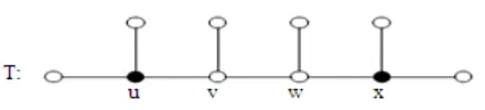
The vertices of small degree play a significant role in determining the degree covering number of a random graph. In particular, it is not necessarily true that if G/ is the random graph obtained from a random graph G by subdividing one edge of G, then γP (G/) = γP (G).
In above Fig. 1, random tree T and T/ are the trees that taken from T by dividing the edge vw once, then γP(T’) > γP(T).
In study (Sharaeh, 2008) Sharaeh investigated about the approximation algorithms for power system monitoring problem solution. We will investigate that the DCS problem is NP-complete even when restricted to bipartite or chordal graphs. We also investigate about linear time algorithm to find a DCS in trees and study theoretical properties of the degree covering number in trees.
NP-completeness: NP-Completeness is one the classic problem in Computer Science that find in many domain in electrical engineering. In this part we discuss the problem of NP-complete even when restricted to bipartite or chordal graphs (Horaka and McAvaneyb, 2007).
Degree Covering Set (Dcs):
Input: A graph G = (V,E) and a positive integer k > 1.
Question: Does G have a DCS of size at most k? Base on the finding on (Kumkratug, 2010) we will make some modifications of the standard proof of NP-completeness of COVERING SET, that able to establish the NP-completeness of the DCS even when restricted to bipartite graphs.
Theorem 5: Degree covering set is NP-complete for bipartite graphs.
Proof: We first show that DCS∈ NP. This is easy to do since one can verify a “yes” input of DCS in polynomial time. That is, for a random graph G = (V,E), a positive integer k and for each subset S∈V with |S| ≤ k, it is easy to verify in polynomial time whether S is a DCS.
We next construct a reduction from NP-complete problem 3-DCS.
The problem of 3-DCS cam be defines follows. Assume we have V = {v1, v2, . . . , vn} as set of variables and a set of 3-element sets K ={K1, K2, . . . , Km}, called clauses, where each clause Ki contains three distinct occurrences of either a variable vi or its complement vi.
Fig. 1: Degree Covering Number of tree equal with 2
Given an input K of 3-DCS, we construct an input G(K) of the DCS as follows. For each variable vi, construct a cycle on four vertices K4, where two nonadjacent vertices are labeled vi and vi. These cycles and vertices are called random cycles and random vertices, respectively. For each clause Kj = {vi, vk, vl} create two nonadjacent vertices labeled Kj,1 and Kj,2 (called clause vertices) and add edges: (vi, Kj,1), (ui, Kj,2), (vk, Kj,1), (vk, Kj,2), (vl, Kj,1), (vl, Kj,2). By construction, the graph G(K) is bipartite.
We will show that K has a satisfying truth assignment if and only if the graph G(K) has a DCS of size at most k = n.
Assume that first that K has a satisfying truth assignment. We create a DCS P in G(K) as follows: Assume that variable vertex vi is map as TRUE and we map variable vertex vi in P; otherwise, put variable vertex vi in P. The set P is a DCS for two reasons: (i) Base on the definition of DCS that v Vertex in each variable cycle K4 belongs to P are dominated. Thus, every edge and vertex in each variable cycle K4 is observed. (ii) Base on Theorem 5 that mention that for every clause vertex Kj is dominated by at least one vertex in P. We can conclude that, all edges between vertex, Kj,1 or Kj,2 and P is a DCS of size at most k = n.
Conversely, we must show that if G(K) has a DCS of size at most k = n, then K has a satisfying truth assignment. Notice first that if P is a DCS of G(K), then it must contain at least one vertex from each variable cycle K4. Therefore, |P| ≥ n, i.e., |P| = n.
Theorem 6: Degree covering set is NP-complete for chordal graphs.
Tree: In this part, we investigate the degree covering number of a tree.
We will define some notations that we will use for the rest of the study.
For any vertex v ∈ V, the nearest neighborhood of v, denoted by N(v), is the set {u ∈ V | uv ∈ E} and its farthest neighborhood N[v] = N(v) ∪ {v}.F or a set S ⊆ V, its nearest neighborhood N(S) = ∪v SN(v) and its farthest neighborhood N[S] = N(S) ⊆ S. The personal neighbor set of a vertex v with respect to a set S, denoted pn[v, S], is the set N[v]-N[S-{v}]. If pn[v, S] ≠ ∅ for some vertex v and some S ⊆ V, then every vertex
of pn[v, S] is called a personal neighbor of v with respect to S, or just an S-pn.
If T is a tree rooted at r and v is a vertex of T, then the level number of v, which we denote by l(v), is the length of the unique r-v path in T. The definition of child and parent will be derived from concept of Tree. A vertex x is a descendant of y (and y is an ancestor of x) if the level lexicographic order of v-w path are monotonically increasing. We let D(v) denote the set of descendants of v and we define D[v] = D(v) ∪ {v}. The maximum of subtree of T rooted at u is the subtree of T induced by D[u] and is denoted by Tu. We defined leaf as an end vertex of T. Downline vertex is a vertex adjacent to a leaf and a vertex adjacent to more than one leave is called a Totally Downline Vertex.
Let T be the tree that divide any number of its edges of any number of times where T has at most one vertex of degree 2 or more. We define that tree as a shade tree.
Theorem 7: For any tree T, γP (T) = 1 if and only if T is a shade tree.
Proof: Suppose T is a shade tree. If T is a path, then any vertex of T forms a DCS in T. On the other hand, if T is not a path, then the vertex of maximum degree in T forms a DCS in T. In any event, γP (T) = 1.This proves the sufficiency.
To prove the necessity, suppose that T is not a shade tree. Then T contains at least two vertices, say u and v, of degree at least 3. We may assume that T is rooted at v. Let S be any DCS of T. If |S| = 1, then, renaming u and v if necessary, we may assume that no vertex in the maximum subtree Tu rooted at u belongs to S.
Base on this explanation, we conclude that, this is contradiction since no edge in Tu.
After this, we will characterize trees T with equal covering and degree covering numbers. We will use the following finding.
Theorem 8: If v is a totally downline vertex in a graph G, then v is in every γ(G)-set and every γP (G).
Proof: Thus assume that γ(T) ≥ 2. Let T be a random tree with γ(T)-set S, where every vertex in S is a totally downline vertex. Then Theorem 8 implies that S is also a unique γP (T)-set. Hence, γP (T) = γ(T).
For some v ∈ S in γ(T)-set S and that v is not a totally downline vertex.
observed by S-{v} and so S-{v} is a DCS for T, contradicting the fact that γP (T) = γ(T). We conclude, |pn[v, S]-{v}| ≥ 1.
From this, we conclude that every vertex in S is a totally downline vertex and S is a unique covering set of T as claimed.
Before proceeding further, we define the shade tree number of a tree T, denoted by stn(T), to be the minimum number of subsets into which V (T) can be partitioned so that each subset induces a shade tree. We call such a partition a shade tree partition and each set of the partition a shade tree subset.
Theorem 9: For random tree T, stn(T) ≤γP (T).
Proof: Suppose m = 1.Then, by Theorem 7, T is a
shade tree and so stn(T) = 1. Suppose, then, that random trees T/ with γP (T/) = m, where m ≥ 1, satisfy stn(T/) ≤γP (T/). Let T be a tree with γP (T) = m + 1.
Let T be a random tree that has root at the vertex vm+1. Our assumption is that v1 is the vertex of S at maximum distance from vm+1 in tree T. Then u1 has at least two neighbors and each neighbor of u1 has degree at most 1 in tree T. Let u1 be the ancestor of v1 of degree at least 3 that is at a minimum distance from v1. It is not difficult to prove that u1 is the neighbor of v1 that has distance with degree 3 in the tree. Thus, stn(T) ≤γP (T).
From above Theorem, we can conclude with this Theorem.
Theorem 10: For any tree T, γP (T) = stn(T).
As a consequence of Theorem 12, we can determine a lower bound on the degree covering of a tree in terms of the number of vertices of degree at least 3.
Theorem 11: If T is a tree having k vertices of degree at:
p
k 2 (T)
3
+
γ ≥
Next we present a linear algorithm for finding a minimum DCS in a nontrivial tree T.
Algorithm FMDCS: Finding Minimum DCS on a non
trivial tree
Input: A tree T on vertices more than 2with the
vertices labeled v1, v2,..., vn so that l(vi) ≤ l(vj) for i > j.
Output: A minimum DCS S of G and a partition of V (G) into |S| subsets {Vx | x ∈ S} so that each subset induces a shade tree.
Begin:
1. If G is a shade tree, then S ← {vn} and Vvn ← V (G) and output S and {Vx | x ∈ S}; otherwise, continue. 2. If degT v ≤ 2, then
2.1. If there exists a child u of v (in G) such that Type(u) = TRUE and u ∈ Vx for some x ∈ S, then
2.1.1. If v is a leaf (in T), then 2.1.1.1. Vx ← Vx ∪ {v},
2.1.1.2. T ← T − v, I ←I \ {i} and go to step 10; 2.1.2. if degT v = 2, then
2.1.2.1. Vx ← Vx ∈ V (Tv), 2.1.2.2. w ← v and go to step 12;
2.2. Otherwise (if no such child exists), I ←I \ {i} and go to step 10;
3. S ← S ∪ {v}. 4. w ← vm,.
5. u ← {child of w on the w-v path}. 6. If w = vn, then
6.1. If the component of T − uw, then output S and {Vx | x ∈ S};
6.2. otherwise, Vn ← V (Tu) and go to step 11. 7. If w /= vn, then
7.1. z ← parent(w);
7.2. If degT w ≥ 4 or if degT w = 3 and the component of T − {uw,wz} containing w is a not a path, then Vv ← V (Tu) and go to step 11;
8. T ← T − V (Tu), I ←I \ {k | vk ∈ V (Tu)} and go to step 13.
9. T ← T − V (Tw), I ← I \ {k | vk ∈ V (Tw)}, Type(w) ← FALSE. Go to step 7.
10. i ← min{k | k ∈ I}.
11. If i <= n, then return to step 4. 12. If i = n, then
End
We now verify the validity of Algorithm FMDCS.
Theorem 12: Algorithm FMDCS produces a γP(G)-set in a nontrivial tree G.
Proof: Let G be a nontrivial tree of order n and let S be the set produced by Algorithm FMDCS. It follows from the way in which the set S is constructed that S is a DCS of G and so γP (G) ≤ |S|. If G is a shade tree, then it follows from Theorem 7 and S = {vn} is a γP(G)-set of G.
RESULTS
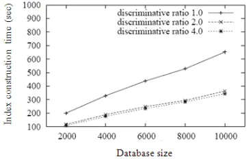
Fig. 2: The scalability of algorithm FMDCS
The scalability of algorithm FMDCS is presented in Fig. 2. We vary the database size from 2000-10000 and construct indexing as the number of minimum DCS from scratch for each database. We also define discriminative ratio thresholds to check how vary the tree inside the graph database.
DISCUSSION
We repeat the experiments for various minimum discriminative ratio thresholds. As shown in the figure, the index construction time is proportional to the database size.
Figure 2 also shows that the indexing construction time does not change too much for a given database when the minimum discriminative ratio is above 2.0. We find that the construction time consists of two parts, frequent graph mining and discriminative feature selection.
CONCLUSION
We consider the graph theoretical representation of this problem as a variation of the covering set problem and define a set S to be a degree covering set of a graph if every vertex and every edge in the system is monitored by the set S (following a set of rules for power system monitoring). The minimum cardinality of a degree covering set of a graph G is the degree covering number γP (G). We show that the Degree Covering Set (DCS) problem is NP-complete even when restricted to bipartite graphs or chordal graphs.
REFERENCES
Ahmadia, A., Y. Alinejad-Beromia and M. Moradib, 2010. Optimal PMU placement for power system observability using binary particle swarm optimization and considering measurement redundancy. Exp. Syst. Appli., 32: 7263-7269. DOI: 10.1016/j.eswa.2010.12.025
Ramos, M.C.G. and C.M.V. Tahan, 2009. An assessment of the electric power quality and electrical installation impacts on medical electrical equipment operations at health care facilities. Am. J. Applied Sci., 6: 638-645. DOI: 10.3844/ajassp.2009.638.645
Kumkratug, P., 2010. Power system stability enhancement using unified power flow controller. Am. J. Applied Sci., 7: 1504-1508. DOI: 10.3844/ajassp.2010.1504.1508
Horaka, P. and K. McAvaneyb, 2007. On covering vertices of a graph by trees. Discrete Math., 308: 4414-4418. DOI: 10.1016/j.disc.2007.08.036 Katrenic, J. and G. Semanisin, 2010. Finding monotone
paths in edge-ordered graphs. Discrete Applied Math., 158: 1624-1632. DOI: 10.1016/j.dam.2010.05.018
Ketabi, A. and S.A. Hosseini, 2008. A new method for optimal harmonic meter placement. Am. J. Applied
Sci., 5: 1499-1505. DOI: 10.3844/ajassp.2008.1499.1505
Pask, D., J. Quigg and I. Raeburn, 2005. Coverings of k-graphs. J. Algebra, 289: 161-191. DOI: 10.1016/j.jalgebra.2005.01.051
Sharaeh, S.H.A., 2008. Random graph generation based p-method and box method for the evaluation of power-aware routing protocols of ad hoc networks. Am. J. Applied Sci., 5: 1662-1669. DOI: 10.3844/ajassp.2008.1662.1669