Fundamentals of Signal
Processing
for Sound and Vibration Engineers
Kihong Shin
Andong National University
Republic of Korea
Joseph K. Hammond
University of Southampton
UK
In July 2006, with the kind support and consideration of Professor Mike Brennan, Kihong Shin managed to take a sabbatical which he spent at the ISVR where his subtle pressures – including attending Joe Hammond’s very last course on signal processing at the ISVR – have distracted Joe Hammond away from his duties as Dean of the Faculty of Engineering, Science and Mathematics.
Thus the text was completed. It is indeed an introduction to the subject and therefore the essential material is not new and draws on many classic books. What we have tried to do is to bring material together, hopefully encouraging the reader to question, enquire about and explore the concepts using the MATLAB exercises or derivatives of them.
It only remains to thank all who have contributed to this. First, of course, the authors whose texts we have referred to, then the decades of students at the ISVR, and more recently in the School of Mechanical Engineering, Andong National University, who have shaped the way the course evolved, especially Sangho Pyo who spent a generous amount of time gath-ering experimental data. Two colleagues in the ISVR deserve particular gratitude: Professor Mike Brennan, whose positive encouragement for the whole project has been essential, to-gether with his very constructive reading of the manuscript; and Professor Paul White, whose encyclopaedic knowledge of signal processing has been our port of call when we needed reassurance.
We would also like to express special thanks to our families, Hae-Ree Lee, Inyong Shin, Hakdoo Yu, Kyu-Shin Lee, Young-Sun Koo and Jill Hammond, for their never-ending support and understanding during the gestation and preparation of the manuscript. Kihong Shin is also grateful to Geun-Tae Yim for his continuing encouragement at the ISVR.
Finally, Joe Hammond thanks Professor Simon Braun of the Technion, Haifa, for his unceasing and inspirational leadership of signal processing in mechanical engineering. Also, and very importantly, we wish to draw attention to a new text written by Simon entitled
Discover Signal Processing: An Interactive Guide for Engineers, also published by John
Wiley & Sons, which offers a complementary and innovative learning experience.
Please note that MATLAB codes (m files) and data files can be downloaded from the Companion Website at www.wiley.com/go/shin hammond
About the Authors
Joe Hammond Joseph (Joe) Hammond graduated in Aeronautical Engineering in 1966 at the University of Southampton. He completed his PhD in the Institute of Sound and Vibration Research (ISVR) in 1972 whilst a lecturer in the Mathematics Department at Portsmouth Polytechnic. He returned to Southampton in 1978 as a lecturer in the ISVR, and was later Senior lecturer, Professor, Deputy Director and then Director of the ISVR from 1992–2001. In 2001 he became Dean of the Faculty of Engineering and Applied Science, and in 2003 Dean of the Faculty of Engineering, Science and Mathematics. He retired in July 2007 and is an Emeritus Professor at Southampton.
CopyrightC 2008 John Wiley & Sons Ltd, The Atrium, Southern Gate, Chichester, West Sussex PO19 8SQ, England
Telephone (+44) 1243 779777
Email (for orders and customer service enquiries): [email protected] Visit our Home Page on www.wileyeurope.com or www.wiley.com
All Rights Reserved. No part of this publication may be reproduced, stored in a retrieval system or transmitted in any form or by any means, electronic, mechanical, photocopying, recording, scanning or otherwise, except under the terms of the Copyright, Designs and Patents Act 1988 or under the terms of a licence issued by the Copyright Licensing Agency Ltd, 90 Tottenham Court Road, London W1T 4LP, UK, without the permission in writing of the Publisher. Requests to the Publisher should be addressed to the Permissions Department, John Wiley & Sons Ltd, The Atrium, Southern Gate, Chichester, West Sussex PO19 8SQ, England, or emailed to [email protected], or faxed to (+44) 1243 770620.
This publication is designed to provide accurate and authoritative information in regard to the subject matter covered. It is sold on the understanding that the Publisher is not engaged in rendering professional services. If professional advice or other expert assistance is required, the services of a competent professional should be sought.
Other Wiley Editorial Offices
John Wiley & Sons Inc., 111 River Street, Hoboken, NJ 07030, USA Jossey-Bass, 989 Market Street, San Francisco, CA 94103-1741, USA Wiley-VCH Verlag GmbH, Boschstr. 12, D-69469 Weinheim, Germany
John Wiley & Sons Australia Ltd, 42 McDougall Street, Milton, Queensland 4064, Australia John Wiley & Sons (Asia) Pte Ltd, 2 Clementi Loop #02-01, Jin Xing Distripark, Singapore 129809 John Wiley & Sons Canada Ltd, 6045 Freemont Blvd, Mississauga, ONT, L5R 4J3
Wiley also publishes its books in a variety of electronic formats. Some content that appears in print may not be available in electronic books.
Library of Congress Cataloging-in-Publication Data
Shin, Kihong.
Fundamentals of signal processing for sound and vibration engineers / Kihong Shin and Joseph Kenneth Hammond.
p. cm.
Includes bibliographical references and index. ISBN 978-0-470-51188-6 (cloth)
1. Signal processing. 2. Acoustical engineering. 3. Vibration. I. Hammond, Joseph Kenneth. II. Title.
TK5102.9.S5327 2007
621.382′2—dc22 2007044557
British Library Cataloguing in Publication Data
A catalogue record for this book is available from the British Library ISBN-13 978-0470-51188-6
Typeset in 10/12pt Times by Aptara, New Delhi, India.
Printed and bound in Great Britain by Antony Rowe Ltd, Chippenham, Wiltshire
This book is printed on acid-free paper responsibly manufactured from sustainable forestry in which at least two trees are planted for each one used for paper production.
MATLABR is a trademark of The MathWorks, Inc. and is used with permission. The MathWorks does not warrant
the accuracy of the text or exercises in this book. This book’s use or discussion of MATLABR software or related
Preface ix
About the Authors xi
1 Introduction to Signal Processing 1
1.1 Descriptions of Physical Data (Signals) 6
1.2 Classification of Data 7
Part I
Deterministic Signals
172 Classification of Deterministic Data 19
2.1 Periodic Signals 19
2.2 Almost Periodic Signals 21
2.3 Transient Signals 24
2.4 Brief Summary and Concluding Remarks 24
2.5 MATLAB Examples 26
3 Fourier Series 31
3.1 Periodic Signals and Fourier Series 31
3.2 The Delta Function 38
3.3 Fourier Series and the Delta Function 41
3.4 The Complex Form of the Fourier Series 42
3.5 Spectra 43
3.6 Some Computational Considerations 46
3.7 Brief Summary 52
3.8 MATLAB Examples 52
4 Fourier Integrals (Fourier Transform) and Continuous-Time Linear Systems 57
4.1 The Fourier Integral 57
4.2 Energy Spectra 61
4.3 Some Examples of Fourier Transforms 62
vi CONTENTS
4.5 The Importance of Phase 71
4.6 Echoes 72
4.7 Continuous-Time Linear Time-Invariant Systems and Convolution 73
4.8 Group Delay (Dispersion) 82
4.9 Minimum and Non-Minimum Phase Systems 85
4.10 The Hilbert Transform 90
4.11 The Effect of Data Truncation (Windowing) 94
4.12 Brief Summary 102
4.13 MATLAB Examples 103
5 Time Sampling and Aliasing 119
5.1 The Fourier Transform of an Ideal Sampled Signal 119
5.2 Aliasing and Anti-Aliasing Filters 126
5.3 Analogue-to-Digital Conversion and Dynamic Range 131
5.4 Some Other Considerations in Signal Acquisition 134
5.5 Shannon’s Sampling Theorem (Signal Reconstruction) 137
5.6 Brief Summary 139
5.7 MATLAB Examples 140
6 The Discrete Fourier Transform 145
6.1 Sequences and Linear Filters 145
6.2 Frequency Domain Representation of Discrete Systems and Signals 150
6.3 The Discrete Fourier Transform 153
6.4 Properties of the DFT 160
6.5 Convolution of Periodic Sequences 162
6.6 The Fast Fourier Transform 164
6.7 Brief Summary 166
6.8 MATLAB Examples 170
Part II
Introduction to Random Processes
1917 Random Processes 193
7.1 Basic Probability Theory 193
7.2 Random Variables and Probability Distributions 198
7.3 Expectations of Functions of a Random Variable 202
7.4 Brief Summary 211
7.5 MATLAB Examples 212
8 Stochastic Processes; Correlation Functions and Spectra 219
8.1 Probability Distribution Associated with a Stochastic Process 220
8.2 Moments of a Stochastic Process 222
8.3 Stationarity 224
8.4 The Second Moments of a Stochastic Process; Covariance
(Correlation) Functions 225
8.5 Ergodicity and Time Averages 229
8.7 Spectra 242
8.8 Brief Summary 251
8.9 MATLAB Examples 253
9 Linear System Response to Random Inputs: System Identification 277
9.1 Single-Input Single-Output Systems 277
9.2 The Ordinary Coherence Function 284
9.3 System Identification 287
9.4 Brief Summary 297
9.5 MATLAB Examples 298
10 Estimation Methods and Statistical Considerations 317
10.1 Estimator Errors and Accuracy 317
10.2 Mean Value and Mean Square Value 320
10.3 Correlation and Covariance Functions 323
10.4 Power Spectral Density Function 327
10.5 Cross-spectral Density Function 347
10.6 Coherence Function 349
10.7 Frequency Response Function 350
10.8 Brief Summary 352
10.9 MATLAB Examples 354
11 Multiple-Input/Response Systems 363
11.1 Description of Multiple-Input, Multiple-Output (MIMO) Systems 363
11.2 Residual Random Variables, Partial and Multiple Coherence Functions 364
11.3 Principal Component Analysis 370
Appendix A Proof of∞−∞2Msin 22πa Mπa Mda=1 375
Appendix B Proof of|Sxy(f)|2≤Sxx(f)Syy(f) 379
Appendix C Wave Number Spectra and an Application 381
Appendix D Some Comments on the Ordinary Coherence Functionγ2
xy(f) 385
Appendix E Least Squares Optimization: Complex-Valued Problem 387
Appendix F Proof ofHW(f)→ H1(f) asκ(f)→ ∞ 389
Appendix G Justification of the Joint Gaussianity ofX(f) 391
Appendix H Some Comments on Digital Filtering 393
References 395
This book has grown out of notes for a course that the second author has given for more years than he cares to remember – which, but for the first author who kept various versions, would never have come to this. Specifically, the Institute of Sound and Vibration Research (ISVR) at the University of Southampton has, for many years, run a Masters programme in Sound and Vibration, and more recently in Applied Digital Signal Processing. A course aimed at introducing students to signal processing has been one of the compulsory mod-ules, and given the wide range of students’ first degrees, the coverage needs to make few assumptions about prior knowledge – other than a familiarity with degree entry-level math-ematics. In addition to the Masters programmes the ISVR runs undergraduate programmes in Acoustical Engineering, Acoustics with Music, and Audiology, each of which to varying levels includes signal processing modules. These taught elements underpin the wide-ranging research of the ISVR, exemplified by the four interlinked research groups in Dynamics, Fluid Dynamics and Acoustics, Human Sciences, and Signal Processing and Control. The large doctoral cohort in the research groups attend selected Masters modules and an acquain-tance with signal processing is a ‘required skill’ (necessary evil?) in many a research project. Building on the introductory course there are a large number of specialist modules ranging from medical signal processing to sonar, and from adaptive and active control to Bayesian methods.
1
Introduction to Signal Processing
Signal processing is the name given to the procedures used on measured data to reveal the information contained in the measurements. These procedures essentially rely on various transformations that are mathematically based and which are implemented using digital tech-niques. The wide availability of software to carry out digital signal processing (DSP) with such ease now pervades all areas of science, engineering, medicine, and beyond. This ease can sometimes result in the analyst using the wrong tools – or interpreting results incorrectly because of a lack of appreciation or understanding of the assumptions or limitations of the method employed.
This text is directed at providing a user’s guide to linear system identification. In order to reach that end we need to cover the groundwork of Fourier methods, random processes, system response and optimization. Recognizing that there are many excellent texts on this,1 why should there be yet another? The aim is to present the material from a user’s viewpoint. Basic concepts are followed by examples and structured MATLAB®exercises allow the user to ‘experiment’. This will not be a story with the punch-line at the end – we actually start in this chapter with the intended end point.
The aim of doing this is to provide reasons and motivation to cover some of the underlying theory. It will also offer a more rapid guide through methodology for practitioners (and others) who may wish to ‘skip’ some of the more ‘tedious’ aspects. In essence we are recognizing that it is not always necessary to be fully familiar with every aspect of the theory to be an effective practitioner. But what is important is to be aware of the limitations and scope of one’s analysis.
1See for example Bendat and Piersol (2000), Brigham (1988), Hsu (1970), Jenkins and Watts (1968), Oppenheim
and Schafer (1975), Otnes and Enochson (1978), Papoulis (1977), Randall (1987), etc.
Fundamentals of Signal Processing for Sound and Vibration Engineers
The Aim of the Book
We are assuming that the reader wishes to understand and use a widely used approach to ‘system identification’. By this we mean we wish to be able to characterize a physical process in a quantified way. The object of this quantification is that it reveals information about the process and accounts for its behaviour, and also it allows us to predict its behaviour in future environments.
The ‘physical processes’ could be anything, e.g. vehicles (land, sea, air), electronic devices, sensors and actuators, biomedical processes, etc., and perhaps less ‘physically based’ socio-economic processes, and so on. The complexity of such processes is unlimited – and being able to characterize them in a quantified way relies on the use of physical ‘laws’ or other ‘models’ usually phrased within the language of mathematics. Most science and engineering degree programmes are full of courses that are aimed at describing processes that relate to the appropriate discipline. We certainly do not want to go there in this book – life is too short! But we still want to characterize these systems – with the minimum of effort and with the maximum effect.
This is where ‘system theory’ comes to our aid, where we employ descriptions or mod-els – abstractions from the ‘real thing’ – that nevertheless are able to capture what may be fundamentally common, to large classes of the phenomena described above. In essence what we do is simply to watch what ‘a system’ does. This is of course totally useless if the system is ‘asleep’ and so we rely on some form of activation to get it going – in which case it is logical to watch (and measure) the particular activation and measure some characteristic of the behaviour (or response) of the system.
In ‘normal’ operation there may be many activators and a host of responses. In most situations the activators are not separate discernible processes, but are distributed. An example of such a system might be the acoustic characteristics of a concert hall when responding to an orchestra and singers. The sources of activation in this case are the musical instruments and singers, the system is the auditorium, including the members of the audience, and the responses may be taken as the sounds heard by each member of the audience.
The complexity of such a system immediately leads one to try and conceptualize something simpler. Distributed activation might be made more manageable by ‘lumping’ things together, e.g. a piano is regarded as several separate activators rather than continu-ous strings/sounding boards all causing accontinu-oustic waves to emanate from each point on their surfaces. We might start to simplify things as in Figure 1.1.
This diagram is a model of a greatly simplified system with several actuators – and the several responses as the sounds heard by individual members of the audience. The arrows indicate a ‘cause and effect’ relationship – and this also has implications. For example, the figure implies that the ‘activators’ are unaffected by the ‘responses’. This implies that there is no ‘feedback’ – and this may not be so.
System
Activators Responses
INTRODUCTION TO SIGNAL PROCESSING 3
System
x(t) y(t)
Figure 1.2 A single activator and a single response system
Having got this far let us simplify things even further to a single activator and a single response as shown in Figure 1.2. This may be rather ‘distant’ from reality but is a widely used model for many processes.
It is now convenient to think of the activatorx(t) and the responsey(t) as time histories. For example,x(t) may denote a voltage, the system may be a loudspeaker andy(t) the pressure at some point in a room. However, this time history model is just one possible scenario. The activatorx may denote the intensity of an image, the system is an optical device andymay be a transformed image. Our emphasis will be on the time history model generally within a sound and vibration context.
The box marked ‘System’ is a convenient catch-all term for phenomena of great variety and complexity. From the outset, we shall impose major constraints on what the box rep-resents – specifically systems that arelinear2 andtime invariant.3 Such systems are very usefully described by a particular feature, namely their response to anideal impulse,4and their corresponding behaviour is then theimpulse response.5 We shall denote this by the symbolh(t).
Because the system is linear this rather ‘abstract’ notion turns out to be very useful in predicting the response of the system to any arbitrary input. This is expressed by the
convolution6of inputx(t) and systemh(t) sometimes abbreviated as
y(t)=h(t)∗x(t) (1.1)
where ‘*’ denotes the convolution operation. Expressed in this form the system box is filled with the characterization h(t) and the (mathematical) mapping or transformation from the inputx(t) to the responsey(t) is the convolution integral.
System identification now becomes the problem of measuringx(t) andy(t) and deducing the impulse response functionh(t). Since we have three quantitative terms in the relationship (1.1), but (assume that) we know two of them, then, in principle at least, we should be able to find the third. The question is: how?
Unravelling Equation (1.1) as it stands is possible but not easy. Life becomes considerably easier if we apply a transformation that maps the convolution expression to a multiplication. One such transformation is theFourier transform.7 Taking theFourier transform of the
convolution8in Equation (1.1) produces
Y(f)=H(f)X(f) (1.2)
*Words in bold will be discussed or explained at greater length later. 2See Chapter 4, Section 4.7.
3See Chapter 4, Section 4.7.
4See Chapter 3, Section 3.2, and Chapter 4, Section 4.7. 5See Chapter 4, Section 4.7.
where f denotes frequency, and X(f),H(f) andY(f) are the transforms ofx(t),h(t) and y(t). This achieves the unravelling of the input–output relationship as a straightforward mul-tiplication – in a ‘domain’ called thefrequency domain.9 In this form the system is char-acterized by the quantity H(f) which is called the system frequency response function (FRF).10
The problem of ‘system identification’ now becomes the calculation of H(f), which seems easy: that is, divideY(f) byX(f), i.e. divide the Fourier transform of the output by the Fourier transform of the input. As long as X(f) is never zero this seems to be the end of the story – but, of course, it is not. Reality interferes in the form of ‘uncertainty’. The measurements x(t) andy(t) are often not measured perfectly – disturbances or ‘noise’ contaminates them – in which case the result of dividing two transforms of contaminated signals will be of limited and dubious value.
Also, the actual excitation signalx(t) may itself belong to a class ofrandom11signals – in which case the straightforward transformation (1.2) also needs more attention. It is this ‘dual randomness’ of the actuating (and hence response) signal and additional contamination that is addressed in this book.
The Effect of Uncertainty
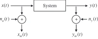
We have referred to randomness or uncertainty with respect to both the actuation and response signal and additional noise on the measurements. So let us redraw Figure 1.2 as in Figure 1.3.
System
+
( )
x t
+
( )
y t
( )
y n t
( )
x n t
( )
m y t
( )
m x t x
Figure 1.3 A single activator/response model with additive noise on measurements
In Figure 1.3,xandydenote the actuation and response signals as before – which may themselves be random. We also recognize thatxandyare usually not directly measurable and we model this by including disturbances written asnxandnywhich add toxandy– so that
the actual measured signals arexmandym. Now we get to the crux of the system identification:
that is, on the basis of (noisy) measurementsxmandym, what is the system?
We conceptualize this problem pictorially. Imagine plotting ym against xm (ignore for
now whatxmandymmight be) as in Figure 1.4.
Each point in this figure is a ‘representation’ of the measured responseymcorresponding
to the measured actuationxm.
System identification, in this context, becomes one of establishing a relationship between ymandxmsuch that it somehow relates to the relationship betweenyandx. The noises are a
INTRODUCTION TO SIGNAL PROCESSING 5
m
x
m
y
Figure 1.4 A plot of the measured signalsymversusxm
nuisance, but we are stuck with them. This is where ‘optimization’ comes in. We try and find a relationship betweenxmandymthat seeks a ‘systematic’ link between the data points which
suppresses the effects of the unwanted disturbances.
The simplest conceptual idea is to ‘fit’ a linear relationship between xm andym. Why
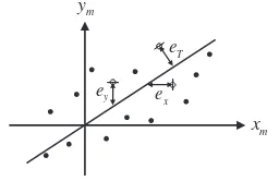
linear? Because we are restricting our choice to the simplest relationship (we could of course be more ambitious). The procedure we use to obtain this fit is seen in Figure 1.5 where the slope of the straight line is adjusted until the match to the data seems best.
This procedure must be made systematic – so we need a measure of how well we fit the points. This leads to the need for a specific measure of fit and we can choose from an unlimited number. Let us keep it simple and settle for some obvious ones. In Figure 1.5, the closeness of the line to the data is indicated by three measures ey,ex andeT. These are regarded as
errors which are measures of the ‘failure’ to fit the data. The quantityey is an error in they
direction (i.e. in the output direction). The quantityexis an error in thexdirection (i.e. in the
input direction). The quantityeT is orthogonal to the line and combines errors in bothxand
ydirections.
We might now look at ways of adjusting the line to minimizeey,ex,eT or some
conve-nient ‘function’ of these quantities. This is now phrased as an optimization problem. A most convenient function turns out to be an average of the squared values of these quantities (‘con-venience’ here is used to reflect not only physical meaning but also mathematical ‘niceness’). Minimizing these three different measures of closeness of fit results in three correspondingly different slopes for the straight line; let us refer to the slopes asmy,mx,mT. So which one
should we use as the best? The choice will be strongly influenced by our prior knowledge of the nature of the measured data – specifically whether we have some idea of the dominant causes of error in the departure from linearity. In other words, some knowledge of the relative magnitudes of the noise on the input and output.
x
e
y
e
T
e
m x m
y
We could look to the figure for a guide:
r
myseems best when errors occur ony, i.e. errors on outputey;
r
mxseems best when errors occur onx, i.e. errors on inputex;
r
mTseems to make an attempt to recognize that errors are on both, i.e.eT.
We might now ask how these rather simple concepts relate to ‘identifying’ the system in Figure 1.3. It turns out that they are directly relevant and lead to three different estimators for the system frequency response function H(f). They have come to be referred to in the literature by the notationH1(f),H2(f)andHT(f),12and are the analogues of the slopesmy,
mx,mT, respectively.
We have now mapped out what the book is essentially about in Chapters 1 to 10. The book ends with a chapter that looks into the implications of multi-input/output systems.
1.1 DESCRIPTIONS OF PHYSICAL DATA (SIGNALS)
Observed data representing a physical phenomenon will be referred to as a time history or a signal. Examples of signals are: temperature fluctuations in a room indicated as a function of time, voltage variations from a vibration transducer, pressure changes at a point in an acoustic field, etc. The physical phenomenon under investigation is often translated by a transducer into an electrical equivalent (voltage or current) and if displayed on an oscilloscope it might appear as shown in Figure 1.6. This is an example of acontinuous(oranalogue) signal.
In many cases, data arediscreteowing to some inherent or imposed sampling procedure. In this case the data might be characterized by a sequence of numbers equally spaced in time. The sampled data of the signal in Figure 1.6 are indicated by the crosses on the graph shown in Figure 1.7.
Time (seconds) Volts
Figure 1.6 A typical continuous signal from a transducer output
X
X
X X X X X
X X
X X
X X X
X
Δseconds
Time (seconds) Volts
Figure 1.7 A discrete signal sampled at everyseconds (marked with×)
CLASSIFICATION OF DATA 7
Spatial position (ξ) Road height
(h)
Figure 1.8 An example of a signal where time is not the natural independent variable
For continuous data we use the notation x(t), y(t), etc., and for discrete data various notations are used, e.g.x(n),x(n),xn (n =0, 1, 2, . . . ).
In certain physical situations, ‘time’ may not be the natural independent variable; for example, a plot of road roughness as a function of spatial position, i.e. h(ξ) as shown in Figure 1.8. However, for uniformity we shall use time as the independent variable in all our discussions.
1.2 CLASSIFICATION OF DATA
Time histories can be broadly categorized as shown in Figure 1.9 (chaotic signals are added to the classifications given by Bendat and Piersol, 2000). A fundamental difference is whether a signal isdeterministicorrandom, and the analysis methods are considerably different depend-ing on the ‘type’ of the signal. Generally, signals are mixed, so the classifications of Figure 1.9 may not be easily applicable, and thus the choice of analysis methods may not be apparent. In many cases some prior knowledge of the system (or the signal) is very helpful for selecting an appropriate method. However, it must be remembered that this prior knowledge (or assump-tion) may also be a source of misleading the results. Thus it is important to remember the First Principle of Data Reduction (Ables, 1974)
The result of any transformation imposed on the experimental data shall incorporate and be consistent with all relevant data and be maximally non-committal with regard to unavailable data.
It would seem that this statement summarizes what is self-evident. But how often do we contravene it – for example, by ‘assuming’ that a time history is zero outside the extent of a captured record?
Signals
Deterministic Random
Periodic Non-periodic Stationary
Transient Almost
periodic
(Chaotic)
Non-stationary
Complex periodic Sinusoidal
m k
x
Figure 1.10 A simple mass–spring system
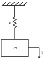
Nonetheless, we need to start somewhere and signals can be broadly classified as being either deterministic or non-deterministic (random). Deterministic signals are those whose behaviour can be predicted exactly. As an example, a mass–spring oscillator is considered in Figure 1.10. The equation of motion ismx¨+kx=0 (xis displacement and ¨xis acceleration). If the mass is released from rest at a positionx(t)=Aand at timet =0, then the displacement signal can be written as
x(t)=Acos
km·t
t≥0 (1.3)
In this case, the displacementx(t) is known exactly for all time. Various types of deter-ministic signals will be discussed later. Basic analysis methods for deterdeter-ministic signals are covered in Part I of this book. Chaotic signals are not considered in this book.
Non-deterministic signals are those whose behaviour cannot be predicted exactly. Some examples are vehicle noise and vibrations on a road, acoustic pressure variations in a wind tunnel, wave heights in a rough sea, temperature records at a weather station, etc. Various terminologies are used to describe these signals, namelyrandom processes(signals),stochastic processes,time series, and the study of these signals is calledtime series analysis. Approaches to describe and analyse random signals require probabilistic and statistical methods. These are discussed in Part II of this book.
The classification of data as being deterministic or random might be debatable in many cases and the choice must be made on the basis of knowledge of the physical situation. Often signals may be modelled as being a mixture of both, e.g. a deterministic signal ‘embedded’ in unwanted random disturbances (noise).
In general, the purpose of signal processing is the extraction of information from a signal, especially when it is difficult to obtain from direct observation. The methodology of extracting information from a signal has three key stages: (i) acquisition, (ii) processing, (iii) interpretation. To a large extent, signal acquisition is concerned withinstrumentation, and we shall treat some aspects of this, e.g.analogue-to-digital conversion.13However, in the main, we shall assume that the signal is already acquired, and concentrate on stages (ii) and (iii).
CLASSIFICATION OF DATA 9
Piezoceramic patch actuator
Slender beam
Accelerometer Force sensor
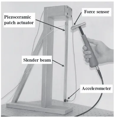
Figure 1.11 A laboratory setup
Some ‘Real’ Data
Let us now look at some signals measured experimentally. We shall attempt to fit the observed time histories to the classifications of Figure 1.9.
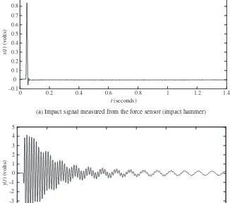
(a) Figure 1.11 shows a laboratory setup in which a slender beam is suspended verti-cally from a rigid clamp. Two forms of excitation are shown. A small piezoceramic PZT (Piezoelectric Zirconate Titanate) patch is used as an actuator which is bonded on near the clamped end. The instrumented hammer (impact hammer) is also used to excite the structure. An accelerometer is attached to the beam tip to measure the response. We shall assume here that digitization effects (ADC quantization,aliasing)14have been adequately taken care of and can be ignored. A sharp tap from the hammer to the structure results in Figures 1.12(a) and (b). Relating these to the classification scheme, we could reasonably refer to these as de-terministic transients. Why might we use the dede-terministic classification? Because we expect replication of the result for ‘identical’ impacts. Further, from the figures the signals appear to be essentially noise free. From a systems points of view, Figure 1.12(a) isx(t) and 1.12(b) is y(t) and from these two signals we would aim to deduce the characteristics of the beam.
(b) We now use the PZT actuator, and Figures 1.13(a) and (b) now relate to a random excitation. The source is a band-limited,15 stationary,16 Gaussian process,17 and in the steady state (i.e. after starting transients have died down) the response should also be stationary. However, on the basis of the visual evidence the response is not evidently stationary (or is it?), i.e. it seems modulated in some way. This demonstrates the difficulty in classification. As it
14See Chapter 5, Sections 5.1–5.3.
15See Chapter 5, Section 5.2, and Chapter 8, Section 8.7. 16See Chapter 8, Section 8.3.
0 0.2 0.4 0.6 0.8 1 1.2 1.4 –0.1
0 0.1 0.2 0.3 0.4 0.5 0.6 0.7 0.8 0.9
t (seconds)
(a) Impact signal measured from the force sensor (impact hammer)
x
(
t
) (volts)
0 0.2 0.4 0.6 0.8 1 1.2 1.4
–5 –4 –3 –2 –1 0 1 2 3 4 5
t (seconds)
(b) Response signal to the impact measured from the accelerometer
y
(
t
) (volts)
Figure 1.12 Example of deterministic transient signals
happens, the response is a narrow-band stationary random process (due to the filtering action of the beam) which is characterized by an amplitude-modulated appearance.
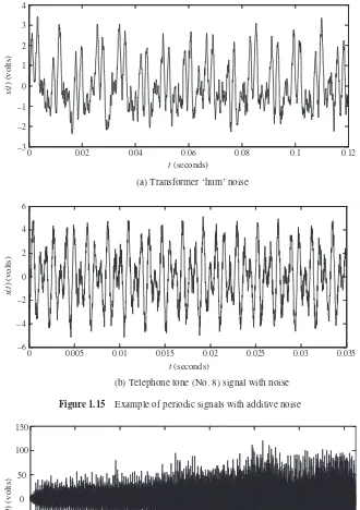
(c) Let us look at a signal from a machine rotating at a constant rate. A tachometer signal is taken from this. As in Figure 1.14(a), this is one that could reasonably be classified as periodic, although there are some discernible differences from period to period – one might ask whether this is simply an additive low-level noise.
(d) Another repetitive signal arises from a telephone tone shown in Figure 1.14(b). The tonality is ‘evident’ from listening to it and its appearance is ‘roughly’ periodic; it is tempting to classify these signals as ‘almost periodic’!
CLASSIFICATION OF DATA 11
0 0.2 0.4 0.6 0.8 1 1.2 1.4 1.6 1.8 2 –3
–2 –1 0 1 2 3
t (seconds)
(a) Input random signal to the PZT (actuator) patch
x
(
t
) (volts)
0 0.2 0.4 0.6 0.8 1 1.2 1.4 1.6 1.8 2 –10
–8 –6 –4 –2 0 2 4 6 8 10
t(seconds)
y
(
t
) (volts)
(b) Response signal to the random excitation measured from the accelerometer
Figure 1.13 Example of stationary random signals
Figure 1.15(b) is a signal created by adding noise (broadband) to the telephone tone signal in Figure 1.14(b). It is not readily apparent that Figure 1.15(b) and Figure 1.15(a) are ‘structurally’ very different.
(f) Figure 1.16(a) is an acoustic recording of a helicopter flyover. The non-stationary structure is apparent – specifically, the increase in amplitude with reduction in range. What is not apparent are any other more complex aspects such as frequency modulation due to movement of the source.
(g) The next group of signals relate to practicalities that occur during acquisition that render the data of limited value (in some cases useless!).
0 0.02 0.04 0.06 0.08 0.1 0.12 0.14 0.16 –0.05
0 0.05
0.1 0.15 0.2
t(seconds)
x
(
t
) (volts)
(a) Tachometer signal from a rotating machine
0 0.005 0.01 0.015 0.02 0.025 0.03 0.035 –5
–4 –3 –2 –1 0 1 2 3 4 5
t(seconds)
x
(
t
) (volts)
(b) Telephone tone (No. 8) signal
Figure 1.14 Example of periodic (and almost periodic) signals
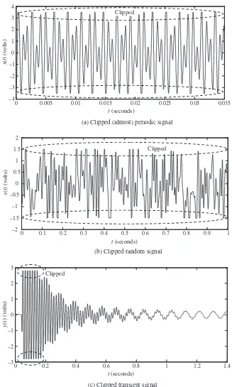
(h) Figures 1.18(a), (b) and (c) all display flats at the top and bottom (positive and negative) of their ranges. This is characteristic of ‘clipping’ or saturation. These have been synthesized by clipping the telephone signal in Figure 1.14(b), the band-limited random signal in Figure 1.13(a) and the accelerometer signal in Figure 1.12(b). Clipping is a nonlinear effect which ‘creates’ spurious frequencies and essentially destroys the credibility of any Fourier transformation results.
CLASSIFICATION OF DATA 13
0 0.02 0.04 0.06 0.08 0.1 0.12
–3 –2 –1 0 1 2 3 4
t(seconds)
x
(
t
) (volts)
(a) Transformer ‘hum’ noise
0 0.005 0.01 0.015 0.02 0.025 0.03 0.035 –6
–4 –2 0 2 4 6
t(seconds)
x
(
t
) (volts)
(b) Telephone tone (No. 8) signal with noise
Figure 1.15 Example of periodic signals with additive noise
0 1 2 3 4 5 6 7
–150 –100 –50
0 50 100 150
t(seconds)
x
(
t
) (volts)
0 0.01 0.02 0.03 0.04 0.05 0.06 0.07 0.08 0.09 –15
–10 –5
0 5 10 15 20
t(seconds)
x
(
t
) (volts)
Figure 1.17 Example of low dynamic range
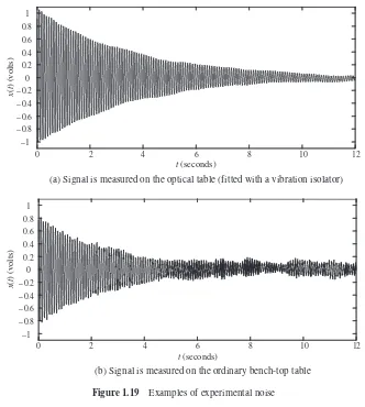
Figure 1.19(b) which we often deal with. Thus, the nature of uncertainty in the measurement process is again emphasized (see Figure 1.3).
The Next Stage
Having introduced various classes of signals we can now turn to the principles and details of how we can model and analyse the signals. We shall use Fourier-based methods – that is, we essentially model the signal as being composed of sine and cosine waves and tailor the processing around this idea. We might argue that we are imposing/assuming some prior information about the signal – namely, that sines and cosines are appropriate descriptors. Whilst this may seem constraining, such a ‘prior model’ is very effective and covers a wide range of phenomena. This is sometimes referred to as anon-parametricapproach to signal processing. So, what might be a ‘parametric’ approach? This can again be related to modelling. We may have additional ‘prior information’ as to how the signal has been generated, e.g. a result of filtering another signal. This notion may be extended from the knowledge that this generation process is indeed ‘physical’ to that of its being ‘notional’, i.e. another model. Specifically Figure 1.20 depicts this whens(t) is the ‘measured’ signal, which is conceived to have arisen from the action of a system being driven by a very fundamental signal – in this case so-called
white noise18w(t).
Phrased in this way the analysis of the signals(t) can now be transformed into a problem of determining the details of the system. The system could be characterized by a set of parameters, e.g. it might be mathematically represented by differential equations and the parameters are the coefficients. Set up like this, the analysis ofs(t) becomes one of system parameter estimation – hence this is a parametric approach.
The system could be linear, time varying or nonlinear depending on one’s prior knowl-edge, and could therefore offer advantages over Fourier-based methods. However, we shall not be pursuing this approach in this book and will get on with the Fourier-based methods instead.
CLASSIFICATION OF DATA 15
0 0.005 0.01 0.015 0.02 0.025 0.03 0.035 –4
–3 –2 –1 0 1 2 3 4
t(seconds)
x
(
t
) (volts)
Clipped
(a) Clipped (almost) periodic signal
0 0.1 0.2 0.3 0.4 0.5 0.6 0.7 0.8 0.9 1 –2
–1.5 –1 –0.5
0 0.5
1 1.5
2
t(seconds)
x
(
t
) (volts)
Clipped
(b) Clipped random signal
0 0.2 0.4 0.6 0.8 1 1.2 1.4
–3 –2 –1 0 1 2 3
t(seconds)
y
(t) (volts)
Clipped
(c) Clipped transient signal
0 2 4 6 8 10 12 –1
–0.8 –0.6 –0.4 –0.2 0 0.2 0.4 0.6 0.8 1
t(seconds)
x
(
t
) (volts)
(a) Signal is measured on the optical table (fitted with a vibration isolator)
0 2 4 6 8 10 12
–1 –0.8 –0.6 –0.4 –0.2 0 0.2 0.4 0.6 0.8 1
t(seconds)
x
(
t
) (volts)
(b) Signal is measured on the ordinary bench-top table
Figure 1.19 Examples of experimental noise
System
w(t) s(t)
Figure 1.20 A white-noise-excited system
Part I
2
Classification of Deterministic Data
Introduction
As described in Chapter 1, deterministic signals can be classified as shown in Figure 2.1. In this figure, chaotic signals are not considered and the sinusoidal signal and more general periodic signals are dealt with together. So deterministic signals are now classified as periodic, almost periodic and transient, and some basic characteristics are explained below.
Transient Almost periodic
Deterministic
Periodic Non-periodic
Figure 2.1 Classification of deterministic signals
2.1 PERIODIC SIGNALS
Periodic signals are defined as those whose waveform repeats exactly at regular time intervals. The simplest example is a sinusoidal signal as shown in Figure 2.2(a), where the time interval for one full cycle is called the period TP (in seconds) and its reciprocal 1/TP is called the
frequency (in hertz). Another example is a triangular signal (or sawtooth wave), as shown in Figure 2.2(b). This signal has an abrupt change (or discontinuity) everyTP seconds. A more
Fundamentals of Signal Processing for Sound and Vibration Engineers
t P
T
(a) Single sinusoidal signal
(c) General periodic signal
(b) Triangular signal
t
P
T
t
P
T
Figure 2.2 Examples of periodic signals
general periodic signal is shown in Figure 2.2(c) where an arbitrarily shaped waveform repeats with periodTP.
In each case the mathematical definition of periodicity implies that the behaviour of the wave is unchanged for all time. This is expressed as
x(t)=x(t+nTP) n= ±1, ±2, ±3, . . . (2.1)
For cases (a) and (b) in Figure 2.2, explicit mathematical descriptions of the wave are easy to write, but the mathematical expression for the case (c) is not obvious. The signal (c) may be obtained by measuring some physical phenomenon, such as the output of an accelerometer placed near the cylinder head of a constant speed car engine. In this case, it may be more useful to consider the signal as being made up of simpler components. One approach to this is to ‘transform’ the signal into the ‘frequency domain’ where the details of periodicities of the signal are clearly revealed. In the frequency domain, the signal is decomposed into an infinite (or a finite) number of frequency components. The periodic signals appear as discrete components in this frequency domain, and are described by a Fourier series which is discussed in Chapter 3. As an example, the frequency domain representation of the amplitudes of the triangular wave (Figure 2.2(b)) with a period of TP =2 seconds is shown in Figure 2.3.
The components in the frequency domain consist of the fundamental frequency 1/TP and its
harmonics 2/TP,3/TP, . . ., i.e. all frequency components are ‘harmonically related’.
ALMOST PERIODIC SIGNALS 21
0 0.5 1 1.5 2 2.5 3 3.5 4 4.5 5
0 0.1 0.2 0.3 0.4 0.5 0.6 0.7 0.8 0.9 1
Frequency (Hz)
|
cn
| (volts) 1
Hz
P T
2
Hz
P T
d.c. (or mean value) component
Figure 2.3 Frequency domain representation of the amplitudes of a triangular wave with a period of
Tp=2
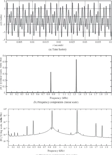
transformed into the frequency domain, we may find something different. The telephone tone of keypad ‘8’ is designed to have frequency components at 852 Hz and 1336 Hz only. This measured telephone tone is transformed into the frequency domain as shown in Figures 2.4(b) (linear scale) and (c) (log scale). On a linear scale, it seems to be composed of the two frequencies. However, there are in fact, many other frequency components that may result if the signal is not perfectly periodic, and this can be seen by plotting the transform on a log scale as in Figure 2.4(c).
Another practical example of a signal that may be considered to be periodic is transformer hum noise (Figure 2.5(a)) whose dominant frequency components are about 122 Hz, 366 Hz and 488 Hz, as shown in Figure 2.5(b). From Figure 2.5(a), it is apparent that the signal is not periodic. However, from Figure 2.5(b) it is seen to have a periodic structure contaminated with noise.
From the above two practical examples, we note that most periodic signals in practical situations are not ‘truly’ periodic, but are ‘almost’ periodic. The term ‘almost periodic’ is discussed in the next section.
2.2 ALMOST PERIODIC SIGNALS
M2.1(This superscript is short for MATLAB Example 2.1)The name ‘almost periodic’ seems self-explanatory and is sometimes called quasi-periodic, i.e. it looks periodic but in fact it is not if observed closely. We shall see in Chapter 3 that suitably selected sine and cosine waves may be added together to represent cases (b) and (c) in Figure 2.2. Also, even for apparently simple situations the sum of sines and cosines results in a wave which never repeats itselfexactly. As an example, consider a wave consisting of two sine components as below
0 0.005 0.01 0.015 0.02 0.025 0.03 0.035 0.04 –5
–3 –1 1 3 5
t (seconds)
(a) Time history
x
(
t
) (volts)
0 0.1 0.2 0.3 0.4 0.5 0.6 0.7 0.8 0.9 1 1.1 1.2 1.3 1.4 1.5 1.6 1.7 1.8 1.9 2 0
0.1 0.2 0.3 0.4 0.5 0.6
Frequency (kHz)
(b) Frequency components (linear scale)
|
X
(
f
)| (linear scale, volts
/
Hz
)
volts
/
Hz
)
10–10 10–8 10–6 10–4 10–2 100
|
X
(
f
)| (log scale,
volts
0 0.1 0.2 0.3 0.4 0.5 0.6 0.7 0.8 0.9 1 1.1 1.2 1.3 1.4 1.5 1.6 1.7 1.8 1.9 2
Frequency (kHz)
(c) Frequency components (log scale)
ALMOST PERIODIC SIGNALS 23
0.01
0 0.02 0.03 0.04 0.05 0.06 0.07 0.08 0.09 0.1 –3
–2 –1 0 1 2 3 4
t (seconds) (a) Time history
x
(
t
) (volts)
0 60 120 180 240 300 360 420 480 540 600 660 720 780 0
0.1 0.2 0.3 0.4 0.5 0.6
Frequency (Hz) (b) Frequency components
|
X
(
f
)| (linear scale, volts/Hz
)
Figure 2.5 Measured transformer hum noise signal
whereA1andA2are amplitudes, p1andp2are the frequencies of each sine component, and θ1andθ2are called the phases. If the frequency ratio p1/p2 is a rational number, the signal x(t) is periodic and repeats at every time interval of the smallest common period of both 1/p1 and 1/p2. However, if the ratiop1/p2is irrational (as an example, the ratiop1/p2=2/
√ 2 is irrational), the signalx(t) never repeats. It can be argued that the sum of two or more sinusoidal components is periodic only if the ratios of all pairs of frequencies are found to be rational numbers (i.e. ratio of integers). A possible example of an almost periodic signal may be an acoustic signal created by tapping a slightly asymmetric wine glass.
basic components here have the form Ae−σtsin(ωt+φ) in which there are four parameters
for each component – namely, amplitudeA, frequencyω, phaseφand an additional featureσ which controls the decay of the component.
Prony analysis fits a sum of such components to the data using an optimization proce-dure. The parameters are found from a (nonlinear) algorithm. The nonlinear nature of the optimization arises because (even ifσ =0) the frequencyωis calculated for each component. This is in contrast to Fourier methods where the frequencies are fixed once the periodTP is
known, i.e. only amplitudes and phases are calculated.
2.3 TRANSIENT SIGNALS
The word ‘transient’ implies some limitation on the duration of the signal. Generally speaking, a transient signal has the property thatx(t)=0 whent → ±∞; some examples are shown in Figure 2.6. In vibration engineering, a common practical example is impact testing (with a hammer) to estimate the frequency response function (FRF, see Equation (1.2)) of a structure. The measured input force signal and output acceleration signal from a simple cantilever beam experiment are shown in Figure 2.7. The frequency characteristic of this type of signal is very different from the Fourier series. The discrete frequency components are replaced by the concept of the signal containing a continuum of frequencies. The mathematical details and interpretation in the frequency domain are presented in Chapter 4.
Note also that the modal characteristics of the beam allow the transient response to be modelled as the sum of decaying oscillations, i.e. ideally matched to the Prony series. This allows the Prony model to be ‘fitted to’ the data (see Davies, 1983) to estimate the amplitudes, frequencies, damping and phases, i.e. a parametric approach.
2.4 BRIEF SUMMARY AND CONCLUDING REMARKS
1. Deterministic signals are largely classified as periodic, almost periodic and transient signals.
2. Periodic and almost periodic signals have discrete components in the frequency domain.
3. Almost periodic signals may be considered as periodic signals having an infinitely long period.
4. Transient signals are analysed using the Fourier integral (see Chapter 4).
BRIEF SUMMARY AND CONCLUDING REMARKS 25
Figure 2.6 Examples of transient signals
0 0.1 0.2 0.3 0.4 0.5 0.6 0.7 0.8 0.9 1
(a) Signal from the force sensor (impact hammer)
(b) Signal from the accelerometer
2.5 MATLAB EXAMPLES
1Example 2.1:Synthesis of periodic signals and almost periodic signals
(see Section 2.2)
Consider Equation (2.2) for this example, i.e.
x(t)=A1sin (2πp1t+θ1)+A2sin (2πp2t+θ2)
Let the amplitudesA1 =A2=1 and phasesθ1=θ2 =0 for convenience.
Case 1: Periodic signal with frequenciesp1=1.4 Hz and p2=1.5 Hz.
Note that the ratio p1/p2 is rational, and the smallest common period of both 1/p1and 1/p2is ‘10’, thus the period is 10 seconds in this case.
Line MATLAB code Comments
1 clear all Removes all local and global variables
(this is a good way to start a new MATLAB script).
2 A1=1; A2=1; Theta1=0; Theta2=0; p1=1.4; p2=1.5;
Define the parameters for Equation (2.2). Semicolon (;) separates statements and prevents displaying the results on the screen.
3 t=[0:0.01:30]; The time variabletis defined as a row vector from zero to 30 seconds with a step size 0.01.
4 x=A1*sin(2*pi*p1*t+Theta1) +A2*sin(2*pi*p2*t+Theta2);
MATLAB expression of Equation (2.2).
5 plot(t, x) Plot the results oftversusx(ton
abscissa andxon ordinate). 6 xlabel('\itt\rm (seconds)');
ylabel('\itx\rm(\itt\rm)')
Add text on the horizontal (xlabel) and on the vertical (ylabel) axes. ‘\it’ is for italic font, and ‘\rm’ is for normal font. Readers may find more ways of dealing with graphics in the section ‘Handle Graphics Objects’ in the MATLAB Help window.
7 grid on Add grid lines on the current figure.
1MATLAB codes (m files) and data files can be downloaded from the Companion Website (www.wiley.com/go/
MATLAB EXAMPLES 27
Results
(a) Periodic signal
0 5 10 15 20 25 30
–2 –1.5 –1 –0.5 0 0.5 1 1.5 2
t(seconds)
x
(
t
)
Comments:It is clear that this signal is periodic and repeats every 10 seconds, i.e. TP =10 seconds, thus the fundamental frequency is 0.1 Hz. The frequency domain
representation of the above signal is shown in Figure (b). Note that the amplitude of the fundamental frequency is zero and thus does not appear in the figure. This ap-plies to subsequent harmonics until 1.4 Hz and 1.5 Hz. Note also that the frequency components 1.4 Hz and 1.5 Hz are ‘harmonically’ related, i.e. both are multiples of 0.1 Hz.
0 0.5 1 1.5 2 2.5 3 3.5 4 4.5 5
0 0.1 0.2 0.3 0.4 0.5
Frequency (Hz)
|
X
(
f
)|
1.4 Hz 1.5 Hz
Case 2: Almost periodic signal with frequenciesp1= √
2 Hz and p2=1.5 Hz. Note that the ratiop1/p2is now irrational, so there is no common period of both 1/p1and 1/p2.
Line MATLAB code Comments
1 clear all
2 A1=1; A2=1; Theta1=0; Theta2=0; p1=sqrt(2); p2=1.5; 3 t=[0:0.01:30];
4 x=A1*sin(2*pi*p1*t+Theta1)
+A2*sin(2*pi*p2*t+Theta2); 5 plot(t, x)
6 xlabel('\itt\rm (seconds)'); ylabel('\itx\rm(\itt\rm)')
7 grid on
Exactly the same script as in the previous case except ‘p1=1.4’ is replaced with ‘p1=sqrt(2)’.
Results
0 5 10 15 20 25 30
–2 –1.5 –1 –0.5 0 0.5 1 1.5 2
t(seconds)
x
(
t
)
(a) Almost periodic signal
MATLAB EXAMPLES 29
frequency components in the signal, but results from the truncation of the signal, i.e. it is a windowing effect (see Sections 3.6 and 4.11 for details).
0 0.5 1 1.5 2 2.5 3 3.5 4 4.5 5 0
0.1 0.2 0.3 0.4 0.5
Frequency (Hz)
|
X
(
f
)|
1.5 Hz
2 Hz
Windowing effect
3
Fourier Series
Introduction
This chapter describes the simplest of the signal types – periodic signals. It begins with the ideal situation and the basis of Fourier decomposition, and then, through illustrative examples, discusses some of the practical issues that arise. The delta function is introduced, which is very useful in signal processing. The chapter concludes with some examples based on the MATLAB software environment.
The presentation is reasonably detailed, but to assist the reader in skipping through to find the main points being made, some equations and text are highlighted.
3.1 PERIODIC SIGNALS AND FOURIER SERIES
Periodic signals are analysed using Fourier series. The basis of Fourier analysis of a periodic signal is the representation of such a signal by adding together sine and cosine functions of appropriate frequencies, amplitudes and relative phases. For a single sine wave
x(t)=Xsin (ωt+φ)=Xsin (2πf t+φ) (3.1)
where X is amplitude,
ω is circular (angular) frequency in radians per unit time (rad/s), f is (cyclical) frequency in cycles per unit time (Hz),
φ is phase angle with respect to thetime originin radians.
The period of this sine wave isTP =1/f =2π/ωseconds. Apositivephase angle φ
shifts the waveform to theleft (a lead or advance) and anegativephase angle to theright (a lag or delay), where the time shift isφ/ωseconds. Whenφ=π/2 the wave becomes a
Fundamentals of Signal Processing for Sound and Vibration Engineers
cosine wave. The Fourier series (for periodic signal) is now described. A periodic signal,x(t), is shown in Figure 3.1 and satisfies
x(t)=x(t+nTP) n= ±1,±2,±3, . . . (3.2)
Figure 3.1 A period signal with a periodTP
With a few exceptions such periodic functions may be represented by
x(t)= a0
The fundamental frequency is f1=1/TP and all other frequencies are multiples
of this.a0/2 is thed.c.level ormean valueof the signal. The reason for wanting to use a representation of the form (3.3) is because it is useful to decompose a ‘complicated’ signal into a sum of ‘simpler’ signals – in this case, sine and cosine waves. The amplitude and phase of each component can be obtained from the coefficientsan,bn, as we shall see
later in Equation (3.12). These coefficients are calculated from the following expressions:
a0
We justify the expressions (3.4) for the coefficientsan,bnas follows. Suppose we wish to
add up a set of ‘elementary’ functionsun(t),n=1,2, . . ., so as to represent a functionx(t), i.e.
we wantncnun(t) to be a ‘good’ representation ofx(t). We may writex(t)≈ncnun(t),
wherecnare coefficients to be found. Note that we cannot assumeequalityin this expression.
PERIODIC SIGNALS AND FOURIER SERIES 33
Since theun(t) are chosen functions,Jis a function ofc1,c2, . . . only, so in order to minimize
Jwe need necessary conditions as below:
∂J ∂cm
=0 for m=1,2, . . . (3.6)
The functionJis
J(c1,c2, . . .)=
and so Equation (3.6) becomes
∂J
Thus the following result is obtained:
TP
At this point we can see that a very desirable property of the ‘basis set’un is that TP
0
un(t)um(t)dt =0 forn=m (3.9)
i.e. they should be ‘orthogonal’.
Assuming this is so, then using the orthogonal property of Equation (3.9) gives the required coefficients as
We began by referring to the amplitude and phase of the components of a Fourier series. This is made explicit now by rewriting Equation (3.3) in the form
x(t)= a0
2 +
∞
n=1
Mncos (2πn f1t+φn) (3.12)
where f1 =1/TP is the fundamental frequency,
Mn=
a2
n+b2nare the amplitudes of frequencies atn f1,
φn =tan−1(−bn/an) are the phases of the frequency components atn f1.
Note that we have assumed that the summation of the components does indeed accurately represent the signal x(t), i.e. we have tacitly assumed the sum converges, and furthermore converges to the signal. This is discussed further in what follows.
An Example (A Square Wave)
As an example, let us find the Fourier series of the function defined by
x(t)= −1 −T
2 <t <0
and x(t+nT)=x(t) n = ±1,±2, . . .
=1 0<t< T 2
(3.13)
where the function can be drawn as in Figure 3.2.
2
T −
2
T t
1
−
1 ( )
x t
0
Figure 3.2 A periodic square wave signal
From Figure 3.2, it is apparent that the mean value is zero, so
a0
2 =
1 T
T/2
−T/2
PERIODIC SIGNALS AND FOURIER SERIES 35
and the coefficientsanandbnare
an =
So Equation (3.13) can be written as
x(t)= 4
We should have anticipated that only a sine wave series is necessary. This follows from the fact that the square wave is an ‘odd’ function and so does not require the cosine terms which are ‘even’ (even and odd functions will be commented upon later in this section). Let us look at the way the successive terms on the right hand side of Equation (3.16) affect the representation. Letω1=2πf1=2π/T, so that
Consider ‘partial sums’ of the series above and their approximation tox(t), i.e. denoted bySn(t), the sum ofnterms, as in Figure 3.3:
n
b
f
1
1
f T=
Figure 3.4 The coefficientsbnof the Fourier series of the square wave
Note the behaviour of the partial sums near points of discontinuity displaying what is known as the ‘overshoot’ orGibbs’phenomenon, which will be discussed shortly. The above Fourier series can be represented in the frequency domain, where it appears as alinespectrum as shown in Figure 3.4.
We now note some aspects of Fourier series.
Convergence of the Fourier Series
We have assumed that a periodic function may be represented by a Fourier series. Now we state (without proof) the conditions (known as the Dirichlet conditions, see Oppenheim et al. (1997) for more details) under which a Fourier series representation is possible. The sufficient conditionsare follows. If a bounded periodic function with periodTP is piecewise
continuous (with a finite number of maxima, minima and discontinuities) in the interval
−TP/2<t ≤TP/2 and has a left and right hand derivative at each pointt0in that interval, then its Fourier series converges. The sum isx(t0) ifxis continuous att0. Ifxis not continuous
att0, then the sum is the average of the left and right hand limits ofxatt0. In the square wave
example above, att=0 the Fourier series converges to
1 2
lim
t→0+x(t)+t→lim0−x(t)
=1
2[1−1]=0
Gibbs’ PhenomenonM3.1
When a function is approximated by a partial sum of a Fourier series, there will be a significant error in the vicinity of a discontinuity, no matter how many terms are used for the partial sum. This is known as Gibbs’ phenomenon.
PERIODIC SIGNALS AND FOURIER SERIES 37
turns out that a lower bound on the overshoot is about 9% of the height of the discontinuity (Oppenheimet al., 1997).
Overshoot
7 Terms 20 Terms
Figure 3.5 Illustrations of Gibbs’ phenomenon
Differentiation and Integration of Fourier Series
If x(t) satisfies the Dirichlet conditions, then its Fourier series may be integrated term by term. Integration ‘smoothes’ jumps and so results in a series whose convergence is enhanced. Satisfaction of the Dirichlet conditions byx(t) does not justify differentiation term by term. But, if periodicx(t) is continuous and its derivative, ˙x(t), satisfies the Dirichlet conditions, then the Fourier series of ˙x(t) may be obtained from the Fourier series ofx(t) by differentiating term by term. Note, however, that these are general guidelines only. Each situation should be considered carefully. For example, the integral of a periodic function for whicha0=0 (mean value of the signal is not zero) is no longer periodic.
Even and Odd Functions
A functionx(t) is even ifx(t)=x(−t), as shown for example in Figure 3.6. A functionx(t) is odd ifx(t)= −x(−t), as shown for example in Figure 3.7. Any functionx(t) may be expressed as the sum of even and odd functions, i.e.
x(t)= 1
2[x(t)+x(−t)]+ 1
2[x(t)−x(−t)]=xe(t)+xo(t) (3.18) Ifx(t) andy(t) are two functions, then the following four properties hold:
1. Ifx(t) is odd andy(t) is odd, thenx(t)·y(t) is even. 2. Ifx(t) is odd andy(t) is even, thenx(t)·y(t) is odd. 3. Ifx(t) is even andy(t) is odd, thenx(t)·y(t) is odd. 4. Ifx(t) is even andy(t) is even, thenx(t)·y(t) is even.
t
t
Figure 3.7 An example of an odd function
Also:
1. Ifx(t) is odd, then −aax(t)dt=0.
2. Ifx(t) is even, then −aax(t)dt =2 0ax(t)dt.
Fourier Series of Odd and Even Functions
Ifx(t) is an odd periodic function with periodTP, then
x(t)=
∞
n=1
bnsin
2πnt
TP
It is a series of odd terms only with a zero mean value, i.e.an=0,n=0, 1, 2, . . . . Ifx(t) is
an even periodic function with periodTP, then
x(t)= a0
2 +
∞
n=1
ancos
2πnt TP
It is now a series of even terms only, i.e.bn=0,n=1, 2, . . . .
We now have a short ‘mathematical aside’ to introduce the delta function, which turns out to be very convenient in signal analysis.
3.2 THE DELTA FUNCTION
The Dirac delta function is denoted byδ(t), and is sometimes called the unit impulse function. Mathematically, it is defined by
δ(t)=0 fort =0, and ∞
−∞
δ(t)dt=1 (3.19)
This is not an ordinary function, but is classified as a ‘generalized’ function. We may consider this function as a very narrow and tall spike att=0 as illustrated in Figure 3.8. Then, Figure 3.8 can be expressed by Equation (3.20), where the integration of the function is −∞∞ δε(t)dt=1. This is a unitimpulse:
δε(t)=
1
ε for −
ε 2 <t <
ε 2
=0 otherwise