Numerical Methods in Engineering with MATLAB

Numerical Methods in Engineering with MATLAB

®

Numerical Methods in Engineering with MATLAB®_{is a text for} engineer-ing students and a reference for practicengineer-ing engineers, especially those who wish to explore the power and efficiency of MATLAB. The choice of numerical methods was based on their relevance to engineering lems. Every method is discussed thoroughly and illustrated with prob-lems involving both hand computation and programming. MATLAB M-files accompany each method and are available on the book web site. This code is made simple and easy to understand by avoiding com-plex book-keeping schemes, while maintaining the essential features of the method. MATLAB, was chosen as the example language because of its ubiquitous use in engineering studies and practice. Moreover, it is widely available to students on school networks and through inexpen-sive educational versions. MATLAB a popular tool for teaching scientific computation.

NUMERICAL METHODS IN

ENGINEERING WITH

MATLAB

®

Jaan Kiusalaas

  

Cambridge, New York, Melbourne, Madrid, Cape Town, Singapore, São Paulo

Cambridge University Press

The Edinburgh Building, Cambridge

 

, UK

First published in print format

-

----

-

----

© Jaan Kiusalaas 2005

2005

Information on this title: www.cambridge.org/9780521852883

This publication is in copyright. Subject to statutory exception and to the provision of

relevant collective licensing agreements, no reproduction of any part may take place

without the written permission of Cambridge University Press.

-

---

-

---

Cambridge University Press has no responsibility for the persistence or accuracy of

s

for external or third-party internet websites referred to in this publication, and does not

guarantee that any content on such websites is, or will remain, accurate or appropriate.

Published in the United States of America by Cambridge University Press, New York

www.cambridge.org

hardback

eBook (NetLibrary)

eBook (NetLibrary)

Contents

Preface . . . .vii

1. Introduction to MATLAB. . . 1

2. Systems of Linear Algebraic Equations. . . 28

3. Interpolation and Curve Fitting. . . .103

4. Roots of Equations. . . .143

5. Numerical Differentiation. . . .182

6. Numerical Integration. . . .200

7. Initial Value Problems. . . .251

8. Two-Point Boundary Value Problems. . . .297

9. Symmetric Matrix Eigenvalue Problems. . . .326

10. Introduction to Optimization. . . .382

Appendices . . . .411

Index . . . .421

Preface

This book is targeted primarily toward engineers and engineering students of ad-vanced standing (sophomores, seniors and graduate students). Familiarity with a computer language is required; knowledge of basic engineering subjects is useful, but not essential.

The text attempts to place emphasis on numerical methods, not programming. Most engineers are not programmers, but problem solvers. They want to know what methods can be applied to a given problem, what are their strengths and pitfalls and how to implement them. Engineers are not expected to write computer code for basic tasks from scratch; they are more likely to utilize functions and subroutines that have been already written and tested. Thus programming by engineers is largely confined to assembling existing pieces of code into a coherent package that solves the problem at hand.

The “piece” of code is usually a function that implements a specific task. For the user the details of the code are unimportant. What matters is the interface (what goes in and what comes out) and an understanding of the method on which the algorithm is based. Since no numerical algorithm is infallible, the importance of understanding the underlying method cannot be overemphasized; it is, in fact, the rationale behind learning numerical methods.

This book attempts to conform to the views outlined above. Each numerical method is explained in detail and its shortcomings are pointed out. The examples that follow individual topics fall into two categories: hand computations that illustrate the inner workings of the method, and small programs that show how the computer code is utilized in solving a problem. Problems that require programming are marked with.

The material consists of the usual topics covered in an engineering course on numerical methods: solution of equations, interpolation and data fitting, numerical differentiation and integration, solution of ordinary differential equations and eigen-value problems. The choice of methods within each topic is tilted toward relevance

viii Preface

to engineering problems. For example, there is an extensive discussion of symmetric, sparsely populated coefficient matrices in the solution of simultaneous equations. In the same vein, the solution of eigenvalue problems concentrates on methods that efficiently extract specific eigenvalues from banded matrices.

An important criterion used in the selection of methods was clarity. Algorithms requiring overly complex bookkeeping were rejected regardless of their efficiency and robustness. This decision, which was taken with great reluctance, is in keeping with the intent to avoid emphasis on programming.

The selection of algorithms was also influenced by current practice. This dis-qualified several well-known historical methods that have been overtaken by more recent developments. For example, the secant method for finding roots of equations was omitted as having no advantages over Brent’s method. For the same reason, the multistep methods used to solve differential equations (e.g., Milne and Adams meth-ods) were left out in favor of the adaptive Runge–Kutta and Bulirsch–Stoer methods.

Notably absent is a chapter on partial differential equations. It was felt that this topic is best treated by finite element or boundary element methods, which are outside the scope of this book. The finite difference model, which is commonly introduced in numerical methods texts, is just too impractical in handling multidimensional boundary value problems.

As usual, the book contains more material than can be covered in a three-credit course. The topics that can be skipped without loss of continuity are tagged with an asterisk (*).

The programs listed in this book were tested with MATLAB® _{6.5.0 and under} Windows®_{XP. The source code can be downloaded from the book’s website at}

www.cambridge.org/0521852889

1

_{Introduction to MATLAB}

1.1

_{General Information}

Quick Overview

This chapter isnotintendedtobeacomprehensivemanual of MATLABR .Oursole

aim is toprovide sufficientinformationtogiveyou a goodstart.Ifyou are familiar withanothercomputerlanguage,and weassume thatyou are,itisnotdifficult topick

uptherestasyou go.

MATLAB isahigh-level computerlanguage forscientific computing and data vi -sualization builtaround an interactiveprogrammingenvironment.Itisbecomingthe

premiereplatformforscientific computing at educationalinstitutionsand research establishments.Thegreatadvantage ofan interactive system is thatprograms can be tested and debuggedquickly,allowingtheuserto concentratemore ontheprinciples

behindtheprogram andless on programming itself. Since thereisnoneedto com

-pile, linkandexecuteaftereach correction, MATLAB programs can bedeveloped in much shortertime thanequivalentFORTRAN or C programs.Onthenegative side, MATLAB doesnotproduce stand-aloneapplications—theprograms can berunonly

oncomputers that have MATLAB installed.

MATLAB has other advantages over mainstreamlanguages that contribute to

rapid program development:

r MATLABcontainsalargenumberof functions thataccessproven numerical li

-braries, suchasLINPACKand EISPACK.Thismeans thatmanycommontasks (e.g., solutionof simultaneous equations) can beaccomplished withasingle function

call.

r Thereis extensivegraphics support thatallows theresults of computations tobe

plotted withafewstatements.

r Allnumerical objectsare treated asdouble-precision arrays.Thus thereisnoneed

todeclaredatatypesandcarryout type conversions.

2 Introduction to MATLAB

The syntaxof MATLAB resembles that ofFORTRAN.Togetan ideaof the similari -ties, letus compare the codeswritten inthe two languages forsolutionof simultaneous equationsAx=bbyGauss elimination.Hereis the subroutinein FORTRAN90:

subroutine gauss(A,b,n)

use prec_mod

implicit none

real(DP), dimension(:,:), intent(in out) :: A

real(DP), dimension(:), intent(in out) :: b

integer, intent(in) :: n

real(DP) :: lambda

integer :: i,k

! ---Elimination

phase---do k = 1,n-1

do i = k+1,n

if(A(i,k) /= 0) then

lambda = A(i,k)/A(k,k)

A(i,k+1:n) = A(i,k+1:n) - lambda*A(k,k+1:n)

b(i) = b(i) - lambda*b(k)

end if

end do

end do

! ---Back substitution

phase---do k = n,1,-1

b(k) = (b(k) - sum(A(k,k+1:n)*b(k+1:n)))/A(k,k)

end do

return

end subroutine gauss

The statementuse prec modtells the compilerto loadthemoduleprec mod

(not shownhere),whichdefines thewordlengthDPfor floating-pointnumbers. Also

note theuse ofarraysections, suchasa(k,k+1:n),afeature thatwasnotavailable

in previousversions ofFORTRAN.

The equivalent MATLABfunction is (MATLAB doesnot have subroutines):

function b = gauss(A,b)

n = length(b);

%---Elimination

phase---for k = 1:n-1

3 1.1 General Information if A(i,k) ˜= 0

lambda = A(i,k)/A(k,k);

A(i,k+1:n) = A(i,k+1:n) - lambda*A(k,k+1:n);

b(i)= b(i) - lambda*b(k);

end

end

end

%---Back substitution

phase---for k = n:-1:1

b(k) = (b(k) - A(k,k+1:n)*b(k+1:n))/A(k,k);

end

Simultaneous equations can alsobe solved inMATLAB with the simple command A_\b(seebelow).

MATLABcan be operated intheinteractivemode throughits command window,

where each command is executed immediately upon its entry.Inthismode MATLAB acts likeanelectronic calculator.Hereisanexample ofan interactive sessionforthe solutionof simultaneous equations:

>> A = [2 1 0; -1 2 2; 0 1 4]; % Input 3 x 3 matrix

>> b = [1; 2; 3]; % Input column vector

>> soln = A\b % Solve A*x = b by left division

soln =

0.2500

0.5000

0.6250

The symbol>>is MATLAB’sprompt for input.Thepercent sign(%)marks the

beginningofacomment. Asemicolon(;) has two functions: it suppressesprintout ofintermediateresultsandseparates the rows ofa matrix. Withoutaterminating

semicolon, theresult ofacommand would bedisplayed. Forexample, omissionof the last semicolon inthe linedefiningthematrixAwould resultin

>> A = [2 1 0; -1 2 2; 0 1 4]

A =

2 1 0

-1 2 2

4 Introduction to MATLAB

Functionsand programs can be created with the MATLABeditor/debugger and

saved with the.mextension(MATLABcalls themM-files).Thefilename ofasaved

functionshould beidentical to thename of the function. Forexample,if the function

forGauss eliminationlisted aboveis saved asgauss.m,it can be called just likeany

MATLABfunction:

>> A = [2 1 0; -1 2 2; 0 1 4];

>> b = [1; 2; 3];

>> soln = gauss(A,b)

soln =

0.2500

0.5000

0.6250

1.2

_{Data Types and Variables}

Data Types

The most commonly used MATLAB data types, orclasses, are double, charand logical, all of which are considered by MATLAB as arrays. Numerical objects

belong to the class double,whichrepresentsdouble-precision arrays; a scalar is treated as a 1×1 array.The elements ofa chartype array are strings (sequences of characters),whereasalogicaltypearrayelementmaycontainonly 1(true) or0 (false).

Another important class isfunction handle,whichisunique to MATLAB.It containsinformation requiredtofind andexecuteafunction.Thename ofafunction

handle consists of the character@, followed bythename of the function;e.g.,@sin. Functionhandlesareused asinputargumentsinfunctioncalls. Forexample, suppose thatwe haveaMATLABfunctionplot(func,x1,x2)thatplotsany user-specified

functionfuncfromx1tox2.The functioncall toplot sinx from0 toπwould be

plot(@sin,0,pi).

Thereare other datatypes,butwe seldomcomeacross them inthis text. Additional classes can bedefined bytheuser.The class ofanobject can bedisplayed with the

classcommand. Forexample,

>> x = 1 + 3i % Complex number

>> class(x)

ans =

5 1.2 Data Types and Variables

Variables

Variablenames,whichmust startwithaletter,arecase sensitive.Hencexstartand xStartrepresent twodifferentvariables.The length of thenameisunlimited,but onlythefirstNcharactersare significant.TofindNfor your installationof MATLAB,

use the commandnamelengthmax:

>> namelengthmax

ans =

63

Variables thatare defined within aMATLAB function are localintheirscope.

They arenotavailable to other parts of theprogram and donotremain in memory afterexitingthe function(thisapplies tomostprogramminglanguages).However,

variables can be shared between afunction andthe calling program if they aredeclared global. Forexample,by placingthe statementglobal X Yin afunction aswellas the calling program, thevariablesXandYare shared betweenthe twoprogram units.

Therecommended practiceis touse capital letters for globalvariables.

MATLABcontains severalbuilt-inconstantsandspecialvariables,mostimportant ofwhichare

ans Defaultname for results

eps Smallestnumberfor which1 + eps > 1

inf Infinity

NaN Nota number

i or j √₋1

pi π

realmin Smallestusablepositivenumber

realmax Largestusablepositivenumber

Hereareafewof examples:

>> warning off % Suppresses print of warning messages

>> 5/0

ans =

Inf

6 Introduction to MATLAB ans =

NaN

>> 5*NaN % Most operations with NaN result in NaN

ans =

NaN

>> NaN == NaN % Different NaN’s are not equal!

ans =

0

>> eps

ans =

2.2204e-016

Arrays

Arrays can be created inseveralways.One of them is to type the elements of thearray between brackets.The elementsineachrow mustbe separated by blanks orcommas.

Hereisanexample ofgenerating a 3×3 matrix:

>> A = [ 2 -1 0

-1 2 -1

0 -1 1]

A =

2 -1 0

-1 2 -1

0 -1 1

The elements can alsobe typedon asingle line, separatingtherowswith semi -colons:

>> A = [2 -1 0; -1 2 -1; 0 -1 1]

A =

2 -1 0

-1 2 -1

0 -1 1

Unlikemost computerlanguages, MATLAB differentiatesbetween row and

7 1.2 Data Types and Variables

>> b = [1 2 3] % Row vector

b =

1 2 3

>> b = [1; 2; 3] % Column vector

b =

1

2

3

>> b = [1 2 3]’ % Transpose of row vector

b =

1

2

3

The single quote (’)is thetranspose operatorinMATLAB;thusb’is the transpose ofb.

The elements ofa matrix, suchas

A=

⎡

⎢ ⎣

A11 A12 A13

A21 A22 A23

A31 A32 A33 ⎤

⎥ ⎦

can beaccessed with the statementA(i,j),whereiandjare therow andcolumn

numbers,respectively. Asectionofan array can be extracted by theuse of colon notation.Hereisan illustration:

>> A = [8 1 6; 3 5 7; 4 9 2]

A =

8 1 6

3 5 7

4 9 2

>> A(2,3) % Element in row 2, column 3

ans =

7

8 Introduction to MATLAB ans =

1

5

9

>> A(2:3,2:3) % The 2 x 2 submatrix in lower right corner

ans =

5 7

9 2

Arrayelements can alsobeaccessed withasingleindex.ThusA(i)extracts the

ith element ofA, countingthe elementsdownthe columns. Forexample,A(7)and A(1,3)wouldextract the same element from a 3×3 matrix.

Cells

Acellarray isasequence ofarbitraryobjects. Cellarrays can be created byenclosing

theircontentsbetween braces{}. Forexample,acellarraycconsistingof three cells can be created by

>> c = {[1 2 3], ’one two three’, 6 + 7i}

c =

[1x3 double] ’one two three’ [6.0000+ 7.0000i]

As seen above, the contents of some cellsarenotprinted inorderto save space.

Ifall contentsare tobedisplayed,use thecelldispcommand:

>> celldisp(c)

c{1} =

1 2 3

c{2} =

one two three

c{3} =

6.0000 + 7.0000i

Bracesarealsousedto extract the contents of the cells:

>> c{1} % First cell

ans =

9 1.3 Operators

>> c{1}(2) % Second element of first cell

ans =

2

>> c{2} % Second cell

ans =

one two three

Strings

Astring isasequence of characters; itis treated byMATLAB asacharacter array. Strings

are created byenclosingthe charactersbetweensingle quotes.They are concatenated with the functionstrcat,whereasacolonoperator(:)isusedto extracta portionof the string. Forexample,

>> s1 = ’Press return to exit’; % Create a string

>> s2 = ’ the program’; % Create another string

>> s3 = strcat(s1,s2) % Concatenate s1 and s2

s3 =

Press return to exit the program

>> s4 = s1(1:12) % Extract chars. 1-12 of s1

s4 =

Press return

1.3

_Operators

Arithmetic Operators

MATLABsupports theusualarithmetic operators:

+ Addition

− Subtraction

∗ Multiplication

ˆ Exponentiation

When appliedtomatrices, they performthe familiar matrixoperations,asillu s-trated below.

>> A = [1 2 3; 4 5 6]; B = [7 8 9; 0 1 2];

10 Introduction to MATLAB ans =

8 10 12

4 6 8

>> A*B’ % Matrix multiplication

ans =

50 8

122 17

>> A*B % Matrix multiplication fails

??? Error using ==> * % due to incompatible dimensions

Inner matrix dimensions must agree.

Thereare twodivisionoperatorsinMATLAB:

/ Rightdivision

\ Leftdivision

Ifaandbare scalars, therightdivisiona/bresultsinadivided byb,whereas the left

division is equivalent to b/a.Inthe casewhereAandBarematrices,A/Breturns the solutionofX*A = BandA_\Byields the solutionofA*X = B.

Often weneedtoapplythe*,/andˆoperations tomatricesin anelement-by -element fashion.This can be doneby precedingthe operator witha period(.)as follows:

.* Element-wisemultiplication

./ Element-wisedivision

.ˆ Element-wise exponentiation

Forexample, the computationCij =AijBijcan beaccomplished with

>> A = [1 2 3; 4 5 6]; B = [7 8 9; 0 1 2];

>> C = A.*B

C =

7 16 27

11 1.3 Operators

Comparison Operators

The comparison(relational) operatorsreturn 1fortrueand0 forfalse.These operators

are

< Less than

> Greaterthan

<= Less thanorequal to

>= Greaterthanorequal to

== Equal to

˜= Not equal to

The comparisonoperatorsalwaysact element-wise on matrices;hence they resultin a matrixoflogicaltype. Forexample,

>> A = [1 2 3; 4 5 6]; B = [7 8 9; 0 1 2];

>> A > B

ans =

0 0 0

1 1 1

Logical Operators

The logical operatorsinMATLAB are

& AND

| OR

˜ NOT

They areusedto build compound relational expressions,an example of whichis shown below.

>> A = [1 2 3; 4 5 6]; B = [7 8 9; 0 1 2];

>> (A > B) | (B > 5)

ans =

1 1 1

12 Introduction to MATLAB

1.4

_{Flow Control}

Conditionals

if, else, elseif

Theifconstruct

if condition block end

executes the blockof statements if thecondition is true.If the condition is false, theblock skipped.Theifconditional can be followed by any numberofelseif

constructs:

if condition block

elseif condition block

.. . end

whichworkinthe samemanner.Theelseclause

.. . else

block end

can beusedtodefine theblock of statementswhichare tobe executed ifnone of theif-elseifclausesare true.The functionsignumbelow illustrates theuse of the conditionals.

function sgn = signum(a)

if a > 0

sgn = 1;

elseif a < 0

sgn = -1;

13 1.4 Flow Control sgn = 0;

end

>> signum (-1.5)

ans =

-1

switch

Theswitchconstructis

switchexpression

casevalue1

block casevalue2

block ..

.

otherwise

block end

Here theexpressionis evaluated andthe controlispassedto thecasethatmatches the

value. For instance,if thevalue ofexpressionis equal tovalue2, theblockof statements following casevalue2is executed. If thevalue ofexpression doesnot matchany

of thecasevalues, the controlpasses to the optionalotherwiseblock.Hereisan

example:

function y = trig(func,x)

switch func

case ’sin’

y = sin(x);

case ’cos’

y = cos(x);

case ’tan’

y = tan(x);

otherwise

error(’No such function defined’)

end

>> trig(’tan’,pi/3)

ans =

14 Introduction to MATLAB

Loops

while

Thewhileconstruct

whilecondition:

block end

executesablockof statementsif theconditionis true. Afterexecutionof theblock,

conditionis evaluated again.Ifitis still true, theblockis executed again.Thisprocess

is continued until theconditionbecomes false.

The followingexample computes thenumberofyearsit takes for a$1000principal togrowto $10,000at6%annualinterest.

>> p = 1000; years = 0;

>> while p < 10000

years = years + 1;

p = p*(1 + 0.06);

end

>> years

years =

40

for

Theforloop requiresatargetand asequenceover which the target loops.The form

of the constructis

for target = sequence block

end

Forexample, to compute cosxfromx=0 toπ /2 atincrements ofπ /10we could use

>> for n = 0:5 % n loops over the sequence 0 1 2 3 4 5

y(n+1) = cos(n*pi/10);

end

>> y

y =

15 1.4 Flow Control

Loops should beavoided whenever possibleinfavorofvectorizedexpressions,

which executemuch faster. A vectorizedsolutionto the last computation would be

>> n = 0:5;

>> y = cos(n*pi/10)

y =

1.0000 0.9511 0.8090 0.5878 0.3090 0.0000

break

Anyloopcan be terminated bythebreakstatement.Uponencountering abreak

statement, the controlispassedto thefirst statement outside the loop.Inthe fol-lowingexample the functionbuildvecconstructsa row vectorofarbitrarylength

by promptingfor its elements.Theprocessis terminated when anemptyelementis encountered.

function x = buildvec

for i = 1:1000

elem = input(’==> ’); % Prompts for input of element

if isempty(elem) % Check for empty element

break

end

x(i) = elem;

end

>> x = buildvec

==> 3

==> 5

==> 7

==> 2

==>

x =

3 5 7 2

continue

Whenthecontinuestatementis encountered in a loop, the controlispassed to thenextiteration without executingthe statementsinthe currentiteration. Asan illustration, considerthe followingfunctionthat stripsall theblanks fromthe strings1:

function s2 = strip(s1)

s2 = ’’; % Create an empty string

16 Introduction to MATLAB if s1(i) == ’ ’

continue

else

s2 = strcat(s2,s1(i)); % Concatenation

end

end

>> s2 = strip(’This is too bad’)

s2 =

Thisistoobad

return

Afunction normally returns to the calling program when itruns out of statements.

However, the functioncan be forcedto exitwith thereturncommand.Inthe ex

-amplebelow, the functionsolveuses the Newton–Raphson methodtofindthe zero of f(x)=sinx−0.5x.Theinput x(guess of the solution)is refined insuccessive

iterationsusingthe formulax←x+x,wherex= −f(x)/f′_{(x),until the change} xbecomes sufficientlysmall.Theprocedureis thenterminated with thereturn

statement.Theforloop assures that thenumberofiterationsdoesnot exceed 30,

which should bemore thanenough forconvergence.

function x = solve(x)

for numIter = 1:30

dx = -(sin(x) - 0.5*x)/(cos(x) - 0.5); % -f(x)/f’(x)

x = x + dx;

if abs(dx) < 1.0e-6 % Check for convergence

return

end

end

error(’Too many iterations’)

>> x = solve(2)

x =

1.8955

error

Executionofa programcan be terminated and a messagedisplayed with theerror

function

error(’message’)

17 1.5 Functions

[m,n] = size(A); % m = no. of rows; n = no. of cols.

if m ˜= n

error(’Matrix must be square’)

end

1.5

_Functions

Function Definition

Thebodyofafunction mustbepreceded bythe function definitionline

function[output args]=function name(input arguments)

Theinput andoutputarguments must be separated bycommas.The numberof

argumentsmay be zero.If thereis onlyone outputargument, the enclosing brackets

may be omitted.

Tomake the function accessible to other programsunits,itmustbe saved under

thefilenamefunction name.m.Thisfilemaycontainotherfunctions, calledsubfunc

-tions.The subfunctions can be calledonly bytheprimaryfunctionfunction nameor

othersubfunctionsinthefile;they arenotaccessible to other program units.

Calling Functions

Afunction may be called with fewer arguments than appear inthe function defini -tion.Thenumberofinputandoutputargumentsused inthe functioncall can be

determined bythe functionsnarginandnargout,respectively.The followingexam

-ple showsa modified versionof the functionsolvethatinvolves twoinputandtwo outputarguments.The errortoleranceepsilonisanoptionalinput thatmay beused

to override thedefaultvalue1.0e-6.The outputargumentnumIter,which contains thenumberofiterations,may alsobe omittedfromthe functioncall.

function [x,numIter] = solve(x,epsilon)

if nargin == 1 % Specify default value if

epsilon = 1.0e-6; % second input argument is

end % omitted in function call

for numIter = 1:100

dx = -(sin(x) - 0.5*x)/(cos(x) - 0.5);

x = x + dx;

if abs(dx) < epsilon % Converged; return to

return % calling program

18 Introduction to MATLAB end

error(’Too many iterations’)

>> x = solve(2) % numIter not printed

x =

1.8955

>> [x,numIter] = solve(2) % numIter is printed

x =

1.8955

numIter =

4

>> format long

>> x = solve(2,1.0e-12) % Solving with extra precision

x =

1.89549426703398

>>

Evaluating Functions

Letus consider aslightly differentversionof the functionsolveshown below.The expressionfordx,namelyx= −f(x)/f′_{(x),isnowcoded inthe functionmyfunc,} so thatsolvecontainsacall tomyfunc.Thiswillworkfine,providedthatmyfuncis stored underthefilenamemyfunc.mso that MATLABcan find it.

function [x,numIter] = solve(x,epsilon)

if nargin == 1; epsilon = 1.0e-6; end

for numIter = 1:30

dx = myfunc(x);

x = x + dx;

if abs(dx) < epsilon; return; end

end

error(’Too many iterations’)

function y = myfunc(x)

y = -(sin(x) - 0.5*x)/(cos(x) - 0.5);

>> x = solve(2)

x =

19 1.5 Functions

Intheaboveversionofsolvethe function returningdxis stuckwith thename

myfunc.Ifmyfuncisreplaced withanotherfunction name,solvewillnotworkunless the correspondingchangeismadein its code.In general,itisnota good ideatoalter

computercode that hasbeentested and debugged; alldatashould be communicated

toa functionthroughitsarguments.MATLAB makes this possibleby passing the functionhandle ofmyfunctosolveasan argument,asillustrated below.

function [x,numIter] = solve(func,x,epsilon)

if nargin == 2; epsilon = 1.0e-6; end

for numIter = 1:30

dx = feval(func,x); % feval is a MATLAB function for

x = x + dx; % evaluating a passed function

if abs(dx) < epsilon; return; end

end

error(’Too many iterations’)

>> x = solve(@myfunc,2) % @myfunc is the function handle

x =

1.8955

The callsolve(@myfunc,2)createsafunctionhandle tomyfuncand passesit tosolveasan argument.Hence thevariable funcinsolvecontains the handle tomyfunc. Afunction passedtoanotherfunction by its handleis evaluated bythe MATLABfunction

feval(function handle,arguments)

It isnow possible tousesolve tofind azero ofany f(x)bycodingthe function

x= −f(x)/f′_{(x)and passing its handle tosolve.}

In-Line Functions

If the function is not overly complicated, it can also be represented as an inline

object:

f unction name=inline(’expression’,’var1’,’var2’,. . .)

whereexpressionspecifies the function andvar1,var2,. . . are thenames of theind

e-pendentvariables.Hereisanexample:

>> myfunc = inline (’xˆ2 + yˆ2’,’x’,’y’);

>> myfunc (3,5)

ans =

20 Introduction to MATLAB

Theadvantage ofan in-line function is thatit can be embedded inthebodyof the code; itdoesnot have toresidein anM-file.

1.6

_Input/Output

Reading Input

The MATLABfunctionfor receiving user inputis

value = input(’prompt’)

Itdisplaysa promptandthen waits for input.If theinputisanexpression,itis evalu

-ated and returned invalue.The followingtwo samplesillustrate theuse ofinput:

>> a = input(’Enter expression: ’)

Enter expression: tan(0.15)

a =

0.1511

>> s = input(’Enter string: ’)

Enter string: ’Black sheep’

s =

Black sheep

Printing Output

Asmentioned before, theresult ofastatementisprinted if the statementdoesnot end withasemicolon.Thisis the easiestwayofdisplaying resultsinMATLAB.Normally

MATLAB displaysnumericalresultswithaboutfivedigits,but this can be changed with the format command:

format long switches to16-digitdisplay

format short switches to5-digitdisplay

Toprint formattedoutput,use thefprintffunction:

fprintf(’format’,list)

where format contains formatting specifications andlist is the list ofitems tobe

21 1.7 Array Manipulation

%w.df Floating pointnotation %w.de Exponentialnotation \n Newline character

wherewis thewidth of thefield anddis thenumberofdigitsafterthedecimalpoint. Linebreakis forced bythenewline character.The followingexampleprintsaformatted

table of sinxvs.xatintervals of 0.2:

>> x = 0:0.2:1;

>> for i = 1:length(x)

fprintf(’%4.1f %11.6f\n’,x(i),sin(x(i)))

end

0.0 0.000000

0.2 0.198669

0.4 0.389418

0.6 0.564642

0.8 0.717356

1.0 0.841471

1.7

_{Array Manipulation}

Creating Arrays

We learned before thatan arraycan be created bytyping its elementsbetween brackets:

>> x = [0 0.25 0.5 0.75 1]

x =

0 0.2500 0.5000 0.7500 1.0000

Colon Operator

Arrayswith equallyspacedelements can alsobe constructed with the colonoperator.

x = first elem:increment:last elem

Forexample,

>> x = 0:0.25:1

x =

22 Introduction to MATLAB

linspace

Another means of creating an array with equallyspacedelementsis thelinspace

function.The statement

x = linspace(xfirst,xlast,n)

createsan arrayofnelements starting withxfirstandending withxlast.Hereisan illustration:

>> x = linspace(0,1,5)

x =

0 0.2500 0.5000 0.7500 1.0000

logspace

The functionlogspaceis the logarithmic counterpart oflinspace.The call

x = logspace(zfirst,zlast,n)

createsnlogarithmicallyspacedelements starting withx=10zf irst_{andending with}

x=10zlast_{.Hereisanexample:}

>> x = logspace(0,1,5)

x =

1.0000 1.7783 3.1623 5.6234 10.0000

zeros

The functioncall

X = zeros(m,n)

returnsa matrixofmrowsandncolumns thatisfilled with zeroes. Whenthe fun -ction is called withasingleargument, e.g.,zeros(n),an×nmatrix is created.

ones

X = ones(m,n)

The functiononesworksinthemanner aszeros,butfills thematrix with ones.

rand

X = rand(m,n)

23 1.7 Array Manipulation

eye

The functioneye

X = eye(n)

createsann×nidentity matrix.

Array Functions

TherearenumerousarrayfunctionsinMATLABthatperform matrixoperationsand

other useful tasks.Hereareafew basic functions:

length

The lengthn(numberof elements) ofa vectorxcan bedetermined with the function length:

n= length(x)

size

If the functionsizeis called withasingleinputargument:

[m,n] = size(X)

itdetermines thenumberofrowsmand numberof columnsninthematrix X.If called with twoinputarguments:

m= size(X,dim)

itreturns the length of Xinthe specified dimension(dim= 1yields thenumberof

rows,anddim=2 gives thenumberof columns).

reshape

Thereshape function isusedtorearrange the elements ofa matrix.The call

Y = reshape(X,m,n)

returnsam×nmatrixthe elements ofwhichare takenfrom matrixXinthe column

-wise order.The totalnumberof elementsin Xmustbe equal tom×n.Hereisan

24 Introduction to MATLAB >> a = 1:2:11

a =

1 3 5 7 9 11

>> A = reshape(a,2,3)

A =

1 5 9

3 7 11

dot

a= dot(x,y)

This function returns thedotproduct of twovectorsxandywhichmustbe of the same length.

prod

a= prod(x)

For a vectorx,prod(x)returns theproduct ofits elements.Ifxisa matrix, thenaisa row vectorcontainingtheproducts overeach column. Forexample,

>> a = [1 2 3 4 5 6];

>> A = reshape(a,2,3)

A =

1 3 5

2 4 6

>> prod(a)

ans =

720

>> prod(A)

ans =

2 12 30

sum

a = sum(x)

25 1.8 Writing and Running Programs

cross

c= cross(a,b)

The functioncrosscomputes the crossproduct:c=a×b,wherevectorsaandb

mustbe of length3.

1.8

_{Writing and Running Programs}

MATLABhas twowindowsavailable fortyping programlines:thecommand window

andtheeditor/debugger.The command window isalwaysintheinteractivemode, so thatanystatement entered into thewindow isimmediately processed.Theinteractive

modeisa good wayto experimentwith the languageandtryoutprogramming ideas.

MATLABopens the editor window when a newM-fileis created, or anexisting file

is opened.The editor window isusedto typeandsaveprograms (calledscriptfilesin

MATLAB)andfunctions.One could alsouseatext editorto enter programlines,but the MATLABeditorhas MATLAB-specific features, suchas colorcoding and automatic

indentation, thatmakework easier. Beforea programorfunctioncan be executed,it

mustbe saved asaMATLABM-file (recall that thesefiles have the.mextension). A programcan berun by invokingtheruncommandfromthe editor’sdebugmenu.

When afunction is calledforthefirst timeduring a program run,itis compiled into P-code (pseudo-code) to speed upexecution insubsequent calls to the function.

One can also create the P-code ofafunction andsaveit on diskby issuingthe command

pcodefunction name

MATLAB will thenloadthe P-code (which has the.pextension)into thememory ratherthanthe textfile.

The variables created during a MATLAB session are saved in the MATLAB

workspaceuntil they are cleared. Listingof the saved variables can bedisplayed bythe commandwho.Ifgreater detailabout thevariablesisrequired, typewhos.Variables can be clearedfromtheworkspacewith the command

cleara b. . .

26 Introduction to MATLAB

Assistance on anyMATLABfunction isavailablebytyping

helpfunction name

inthe command window.

1.9

_Plotting

MATLABhas extensiveplottingcapabilities.Hereweillustrate somebasic commands fortwo-dimensionalplots.The examplebelow plots sinxandcosxonthe sameplot.

>> x = 0:0.2:pi; % Create x-array

>> y = sin(x); % Create y-array

>> plot(x,y,’k:o’) % Plot x-y points with specified color

% and symbol (’k’ = black, ’o’ = circles)

>> hold on % Allow overwriting of current plot

>> z = cos(x); % Create z-array

>> plot(x,z,’k:x’) % Plot x-z points (’x’ = crosses)

>> grid on % Display coordinate grid

>> xlabel(’x’) % Display label for x-axis

>> ylabel(’y’) % Display label for y-axis

>> gtext(’sin x’) % Create mouse-movable text

27 1.9 Plotting

Afunctionstored in aM-file can beplotted withasingle command,as shown below.

function y = testfunc(x) % Stored function

y = (x.ˆ3).*sin(x) - 1./x;

>> fplot(@testfunc,[1 20]) % Plot from x = 1 to 20

>> grid on

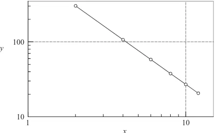
Theplotsappearing inthisbook fromhere on werenotproduced byMATLAB. Weusedthe copy/paste operationto transferthenumericaldatatoaspreadsheet

2

_{Systems of Linear Algebraic Equations}

Solve the simultaneous equationsAx=b

2.1

_Introduction

Inthis chapter we lookat the solutionofnlinear,algebraic equationsinnunknowns.

It is byfarthe longest and arguably themostimportant topicin thebook.There

is a good reasonforthis—itis almost impossible to carryoutnumerical analysis ofanysortwithout encounteringsimultaneous equations.Moreover, equationsets

arisingfrom physicalproblems are often verylarge, consuming alot of computa -tionalresources.Itusually possible toreduce the storagerequirementsandtherun

time byexploiting specialproperties of the coefficientmatrix, suchas sparseness (most elements ofasparsematrix are zero).Hence therearemany algorithmsded

-icatedto the solutionof large sets of equations, each onebeingtailoredtoa parti

c-ularformof the coefficientmatrix(symmetric,banded, sparse, etc.). A well-known

collectionof theseroutinesisLAPACK –Linear AlgebraPACKage, originally written in Fortran771_.

We cannotpossibly discussall the specialalgorithmsinthe limitedspaceavai

l-able.Thebestwe can dois topresent thebasicmethods of solution, supplemented by afew usefulalgorithms for banded andsparse coefficientmatrices.

Notation

Asystemofalgebraic equations has the form

1 _{LAPACKis the successorofLINPACK,a 1970sand 80s collectionofFortransubroutines.}

30 Systems of Linear Algebraic Equations

secondequation.Thenumberof such combinationsisinfinite.Onthe otherhand, the equations

2x+y=3 4x+2y=0

haveno solution because the secondequation,beingequivalent to2x+y=0, con -tradicts thefirst one.Therefore,anysolutionthat satisfies one equationcannot satisfy

the otherone.

Ill-Conditioning

Anobvious question is: what happenswhenthe coefficientmatrix isalmost singular; i.e.,if|A|isverysmall? Inordertodeterminewhetherthedeterminant of the coefficient

matrix is“small,” weneed a referenceagainstwhich thedeterminant can bemeasured.

Thisreferenceis calledthenormof thematrix,denoted byA. We canthensaythat thedeterminantis smallif

|A|<<A

Severalnorms ofa matrixhavebeen defined inexistingliterature, suchas

A =

n

i=1

n

j=1

A2

ij A =₁max

≤i≤n n

j=1 A_ij

(2.5a)

Aformalmeasure of conditioning is thematrixcondition number,defined as

cond(A)= AA−1

(2.5b)

If thisnumber is close tounity, thematrix iswell-conditioned.The condition number increaseswith thedegree ofill-conditioning,reaching infinityfor asingular matrix.

Note that the condition number isnotunique,butdepends onthe choice of thematrix norm.Unfortunately, the condition number is expensive to compute forlargematri -ces.In most casesitis sufficient togauge conditioning bycomparingthedeterminant

with themagnitudes of the elementsinthematrix.

If the equationsareill-conditioned, small changesinthe coefficientmatrix result

inlarge changesinthe solution. Asan illustration, considerthe equations

2x+y=3 2x+1.001y=0

that have the solutionx=1501.5,y= −3000. Since|A| =2(1.001)−2(1)=0.002 is

much smallerthanthe coefficients, the equationsareill-conditioned.The effect of

ill-conditioningcan beverified bychangingthe secondequationto2x+1.002y=0

31 2.1 Introduction

Numerical solutions ofill-conditionedequationsarenot tobe trusted.Thereason is that theinevitableroundoff errorsduringthe solution processare equivalent toin -troducingsmall changesinto the coefficientmatrix.Thisinturn introduces large errors

into the solution, themagnitude ofwhichdepends onthe severityofill-conditioning.

Insuspect cases thedeterminant of the coefficientmatrixshould be computedso that thedegree ofill-conditioningcan be estimated.This can bedoneduringor afterthe solution with only asmall computational effort.

Linear Systems

Linear,algebraic equations occur in almostallbranches ofnumericalanalysis. But their mostvisibleapplication inengineering isintheanalysis of linearsystems (any

system whoseresponseisproportional to theinputisdeemedtobe linear). Linear

systemsinclude structures, elastic solids, heatflow, seepage offluids, electromagnetic

fieldsandelectric circuits; i.e.,most topics taughtin anengineeringcurriculum.

If the system isdiscrete, suchasatruss or anelectric circuit, then itsanalysis leadsdirectly to linear algebraic equations.Inthe case of astatically determinate truss, forexample, the equationsarisewhenthe equilibriumconditions of thejoints

arewritten down.Theunknownsx1,x2, . . . ,xnrepresent the forcesinthemembers

andthe supportreactions,andthe constantsb1,b2, . . . ,bnare theprescribedexternal loads.

Thebehaviorof continuous systemsisdescribed by differential equations,rather

than algebraic equations.However,becausenumericalanalysis can deal only with

discretevariables,itisfirstnecessarytoapproximatea differential equation witha

systemofalgebraic equations.Thewell-known finitedifference,finite elementand boundaryelementmethods ofanalysisworkinthismanner.They usedifferentap

-proximations toachieve the“discretization,” butineach case thefinal taskis the same:

solveasystem(often a verylarge system) of linear,algebraic equations.

Insummary, themodelingof linearsystemsinvariably givesrise to equations of the formAx=b,wherebis theinputandxrepresents theresponse of the system.

The coefficientmatrixA,whichreflects the characteristics of the system,isind

e-pendent of theinput.Inother words,if theinputis changed, the equations have to

be solved again witha differentb,but the sameA.Therefore,itisdesirable to have

anequation-solving algorithmthat canhandleany numberof constantvectorswith

minimal computational effort.

Methods of Solution

32 Systems of Linear Algebraic Equations

transformthe original equationsintoequivalent equations(equations that have the same solution) that can be solved more easily.The transformation is carriedoutby applyingthe three operations listed below.These so-calledelementary operationsdo

not change the solution,but they may affect thedeterminant of the coefficientmatrix asindicated in parentheses.

r Exchangingtwo equations (changes signof

|A|).

r Multiplying an equation by a nonzero constant (multiplies |A| by the same

constant).

r Multiplying anequation by a nonzero constantandthensubtracting it from an

-otherequation(leaves|A|unchanged).

Iterative, orindirect methods, startwitha guess of the solutionx,andthen r

e-peatedly refine the solution untilacertainconvergence criterion isreached.Iterative

methodsaregenerallyless efficient thantheir direct counterpartsdue to the large

numberofiterationsrequired. But they do have significant computationaladvan -tagesif the coefficientmatrix isverylargeandsparsely populated(most coefficients

are zero).

Overview of Direct Methods

Table2.1lists threepopular directmethods, each ofwhichuses elementaryoperations toproduceits own final formof easy-to-solve equations.

Method Initial form Final form

Gauss elimination Ax=b Ux=c

LUdecomposition Ax=b LUx=b

Gauss–Jordanelimination Ax=b Ix=c

Table 2.1

Intheabove tableUrepresentsan uppertriangular matrix,Lisalowertriangular matrix andI denotes the identity matrix. Asquarematrix is called triangularifit contains onlyzero elements onone side of the leading diagonal.Thusa 3×3 upper

triangular matrixhas the form

U=

⎡

⎢ ⎣

U11 U12 U13

0 U22 U23

0 0 U33 ⎤

33 2.1 Introduction

and a 3×3lowertriangular matrix appearsas

L=

⎡

⎢ ⎣

L11 0 0

L21 L22 0

L31 L32 L33 ⎤

⎥ ⎦

Triangular matricesplay an importantroleinlinear algebra, since theysimplify manycomputations. Forexample, considerthe equationsLx=c, or

L11x1 =c1

L21x1+L22x2 =c2

L31x1+L32x2+L33x3 =c3

.. .

Ifwe solve the equations forward, starting with thefirst equation, the computations

areveryeasy, since each equation wouldcontainonlyoneunknown atatime.The solution wouldthusproceed as follows:

x1 =c1/L11

x2 =(c2−L21x1)/L22

x3 =(c3−L31x1−L32x2)/L33

.. .

Thisprocedureis known asforward substitution.In asimilar way,Ux=c,encountered inGauss elimination, caneasily be solved bybacksubstitution,which startswith the last equation and proceedsbackwardthrough the equations.

The equationsLUx=b,whichareassociated withLUdecomposition, can also

be solvedquickly ifwereplace them with two sets of equivalent equations:Ly=b

andUx=y.NowLy=bcan be solvedforybyforwardsubstitution, followed bythe solutionofUx=yby means ofback substitution.

The equations Ix=c, which are produced by Gauss–Jordan elimination, are equivalent tox=c(recall theidentityIx=x), so thatcisalreadythe solution.

EXAMPLE 2.1

Determinewhetherthe following matrix is singular:

A=

⎡

⎢ ⎣

2.1 −0.6 1.1 3.2 4.7 −0.8 3.1 −6.5 4.1

⎤

35 2.2 Gauss Elimination Method

theprocedure, letus solve the equations

4x1−2x2+x3=11 (a)

−2x1+4x2−2x3= −16 (b)

x1−2x2+4x3=17 (c)

Elimination phase The elimination phaseutilizes onlyone of the elementaryop -erations listed inTable2.1—multiplyingone equation(say, equationj)by aconstant

λandsubtracting it from anotherequation(equationi).The symbolicrepresentation

of this operation is

Eq.(i)←Eq.(i)−λ× Eq.(j) (2.6)

The equation beingsubtracted,namely Eq.(j),is calledthepivot equation.

We start the elimination bytaking Eq.(a) tobe thepivot equation andchoosing

themultipliersλsoas to eliminatex1from Eqs.(b)and(c):

Eq.(b)←Eq.(b)−(−0.5)×Eq.(a)

Eq.(c)←Eq.(c)−0.25×Eq.(a)

Afterthis transformation, the equationsbecome

4x1−2x2+x3=11 (a)

3x2−1.5x3= −10.5 (b)

−1.5x2+3.75x3=14.25 (c)

This completes thefirstpass.Now wepick (b)as thepivot equation andeliminatex2

from(c):

Eq.(c)←Eq.(c)−(−0.5)×Eq.(b)

whichyields the equations

4x1−2x2+x3=11 (a)

3x2−1.5x3= −10.5 (b)

3x3=9 (c)

The elimination phaseisnowcomplete.The original equations havebeen replaced byequivalent equations that can be easilysolved by back substitution.

Aspointed outbefore, theaugmented coefficientmatrix isa more convenient

36 Systems of Linear Algebraic Equations written as

⎡

⎢ ⎣

4 −2 1 11

−2 4 −2 −16

1 −2 4 17

⎤

⎥ ⎦

andthe equivalent equationsproduced bythefirstandthe second passes of Gauss elimination would appear as

⎡

⎢ ⎣

4 −2 1 11.00 0 3 −1.5 −10.50 0 −1.5 3.75 14.25

⎤

⎥ ⎦

⎡

⎢ ⎣

4 −2 1 11.0 0 3 −1.5 −10.5

0 0 3 9.0

⎤

⎥ ⎦

It is important to note that the elementary row operation in Eq.(2.6) leaves thedeterminant of the coefficientmatrix unchanged.Thisisratherfortunate, since thedeterminant ofa triangular matrix is veryeasy to compute—itis the product of thediagonal elements (youcan verifythis quite easily).Inother words,

|A| = |U| =U11×U22× · · · ×Unn (2.7)

Back substitution phase Theunknowns can now be computed by back substitu -tion inthemanner described inthepreviousarticle. Solving Eqs.(c), (b)and(a)in

that order,weget

x3=9/3=3

x2=(−10.5+1.5x3)/3=[−10.5+1.5(3)]/3= −2

x1=(11+2x2−x3)/4=[11+2(−2)−3]/4=1

Algorithm for Gauss Elimination Method

Elimination phase Letus lookat the equationsat someinstantduringthe elim

-ination phase. Assume that thefirstkrows ofAhavealready beentransformedto

uppertriangularform.Therefore, the currentpivot equation is thekth equation,and all the equationsbelow itare still tobe transformed.This situation isdepicted bythe

augmentedcoefficientmatrixshown below.Note that the components ofAarenot the coefficients of the original equations (except forthefirstrow), since theyhave

38 Systems of Linear Algebraic Equations

the lower triangular portion of the coefficient matrix anyway, its contents are

irrelevant.

Back substitution phase AfterGauss eliminationtheaugmentedcoefficientma -trixhas the form

A b

=

⎡

⎢ ⎢ ⎢ ⎢ ⎢ ⎢ ⎣

A11 A12 A13 · · · A1n b1

0 A22 A23 · · · A2n b2

0 0 A33 · · · A3n b3

..

. ... ... ... ...

0 0 0 · · · Ann bn

⎤

⎥ ⎥ ⎥ ⎥ ⎥ ⎥ ⎦

The last equation,Annxn=bn,is solved first,yielding

xn=bn/Ann (2.9)

Consider nowthe stage ofback substitution wherexn,xn−1, . . . ,xk+1havebeen

already beencomputed(inthat order),and weareabout todeterminexkfromthekth equation

Akkxk+Ak,k+1xk+1+ · · · +Aknxn=bk

The solution is

xk=

bk−

n

j=k+1

Ak jxj

1

Akk, k=n−1,n−2, . . . ,1 (2.10)

The corresponding algorithmfor back substitution is:

for k = n:-1:1

b(k) = (b(k) - A(k,k+1:n)*b(k+1:n))/A(k,k);

end

gauss

The functiongausscombines the elimination andtheback substitution phases. Dur

-ing back substitutionbis overwritten bythe solution vectorx, so thatbcontains the solution uponexit.

function [x,det] = gauss(A,b)

% Solves A*x = b by Gauss elimination and computes det(A).

% USAGE: [x,det] = gauss(A,b)

if size(b,2) > 1; b = b’; end % b must be column vector

39 2.2 Gauss Elimination Method

for k = 1:n-1 % Elimination phase

for i= k+1:n

if A(i,k) ˜= 0

lambda = A(i,k)/A(k,k);

A(i,k+1:n) = A(i,k+1:n) - lambda*A(k,k+1:n);

b(i)= b(i) - lambda*b(k);

end

end

end

if nargout == 2; det = prod(diag(A)); end

for k = n:-1:1 % Back substitution phase

b(k) = (b(k) - A(k,k+1:n)*b(k+1:n))/A(k,k);

end

x = b;

Multiple Sets of Equations

As mentioned before,it is frequently necessary to solve the equations Ax=b for

several constant vectors. Let there be m such constant vectors, denoted by

b1,b2, . . . ,bmandlet the correspondingsolution vectorsbex1,x2, . . . ,xm. Wedenote

multiple sets of equationsbyAX=B,where

X=

x1 x2 · · · xm

B=

b1 b2 · · · bm

aren×mmatriceswhose columns consist of solution vectorsandconstantvectors,

respectively.

Aneconomicalwayto handle such equationsduringthe elimination phaseis toincludeallmconstantvectorsintheaugmentedcoefficientmatrix, so that they are transformedsimultaneously with the coefficientmatrix.The solutionsare then

obtained by back substitution intheusualmanner, onevector atatime.Itwouldquite easytomake the correspondingchangesingauss.However, theLUdecomposition method,described inthenextarticle,ismoreversatileinhandling multiple constant

vectors.

EXAMPLE 2.3

Use Gauss eliminationto solve the equationsAX=B,where

A=

⎡

⎢ ⎣

6 −4 1

−4 6 −4

1 −4 6

⎤

⎥

⎦ B=

⎡

⎢ ⎣

−14 22 36 −18

6 7

⎤

41 2.2 Gauss Elimination Method

EXAMPLE 2.4

Ann×nVandermodematrixAisdefined by

Aij=vin−j, i=1,2, . . . ,n, j=1,2, . . . ,n

wherevisa vector.InMATLAB aVandermodematrixcan begenerated bythe com

-mandvander(v).Use the functiongaussto compute the solutionofAx=b,where

Ais the6×6Vandermodematrix generatedfromthevector

v=

1.0 1.2 1.4 1.6 1.8 2.0T

and

b=

0 1 0 1 0 1

T

Also evaluate the accuracy of the solution(Vandermode matrices tend to be i ll-conditioned).

Solution Weusedtheprogramshown below. AfterconstructingAandb, the output formatwas changedto longso that the solution would beprinted to14decimal

places.Hereare theresults:

% Example 2.4 (Gauss elimination)

A = vander(1:0.2:2);

b = [0 1 0 1 0 1]’;

format long

[x,det] = gauss(A,b)

x =

1.0e+004 *

0.04166666666701

-0.31250000000246

0.92500000000697

-1.35000000000972

0.97093333334002

-0.27510000000181

det =

-1.132462079991823e-006

As thedeterminantis quite smallrelative to the elements ofA(you may want to

printAtoverifythis),we expectdetectableroundoff error.Inspectionofxleadsus to suspect that the exact solution is

x=

1250/3 −3125 9250 −13500 29128/3 −2751T

42 Systems of Linear Algebraic Equations

Another waytogauge theaccuracyof the solution is to computeAxandcompare theresult tob:

>> A*x

ans =

-0.00000000000091

0.99999999999909

-0.00000000000819

0.99999999998272

-0.00000000005366

0.99999999994998

Theresult seems to confirmour previous conclusion.

2.3

_{LU Decomposition Methods}

Introduction

Itispossible to showthatanysquarematrixAcan be expressed asa product ofalower

triangular matrixLand an uppertriangular matrixU:

A=LU (2.11)

Theprocess of computingLandUfor a givenAis known asLUdecompositionor

LUfactorization. LUdecomposition isnotunique (the combinations ofLandUfor a prescribedAare endless),unless certainconstraintsareplacedonLorU.These constraintsdistinguish one type ofdecompositionfrom another.Three commonly used decompositionsare listed inTable2.2.

Name Constraints

Doolittle’sdecomposition Lii=1, i=1,2, . . . ,n

Crout’sdecomposition Uii=1, i =1,2, . . . ,n

Choleski’sdecomposition L=UT

Table 2.2

After decomposingA,itis easyto solve the equationsAx=b,aspointedoutin Art. 2.1. Wefirstrewrite the equationsasLUx=b.Upon usingthenotationUx=y, the equationsbecome

43 2.3 LU Decomposition Methods

which can be solvedforybyforwardsubstitution.Then

Ux=y

willyieldxbytheback substitution process.

Theadvantage ofLUdecompositionoverthe Gauss elimination method is that onceAisdecomposed,we cansolveAx=bfor asmanyconstantvectorsbaswe

please.The cost of eachadditional solution isrelativelysmall, since the forward and back substitutionoperationsaremuch less time consumingthanthedecomposition process.

Doolittle’s Decomposition Method

Decomposition phase Doolittle’sdecomposition is closely relatedto Gauss elim

-ination.Inordertoillustrate therelationship, consider a 3×3 matrixAand assume that there exist triangular matrices

L=

⎡

⎢ ⎣

1 0 0

L21 1 0

L31 L32 1 ⎤

⎥

⎦ U=

⎡

⎢ ⎣

U11 U12 U13

0 U22 U23

0 0 U33 ⎤

⎥ ⎦

such thatA=LU. Aftercompletingthemultiplicationontheright handside,weget

A=

⎡

⎢ ⎣

U11 U12 U13

U11L21 U12L21+U22 U13L21+U23

U11L31 U12L31+U22L32 U13L31+U23L32+U33 ⎤

⎥

⎦ (2.12)

Letusnow applyGauss eliminationtoEq.(2.12).Thefirstpass of the elimina -tion procedure consists of choosingthefirstrow as thepivotrow and applyingthe elementaryoperations

row 2←row 2−L21×row 1(eliminates A21)

row 3←row 3−L31×row 1(eliminates A31)

Theresultis

A′=

⎡

⎢ ⎣

U11 U12 U13

0 U22 U23

0 U22L32 U23L32+U33 ⎤

⎥ ⎦

Inthenextpasswe take the second row as thepivotrow,and utilize the operation

44 Systems of Linear Algebraic Equations

ending up with

A′′=U=

⎡

⎢ ⎣

U11 U12 U13

0 U22 U23

0 0 U33 ⎤

⎥ ⎦

The foregoing illustration reveals twoimportant features ofDoolittle’sdecomp o-sition:

r ThematrixUisidentical to theuppertriangular matrixthatresults fromGauss

elimination.

r The off-diagonal elements ofLare thepivot equation multipliersused during

Gauss elimination;thatis,Lijis themultiplierthat eliminatedAij.

Itisusualpractice to store themultipliersinthe lowertriangular portionof the coefficientmatrix,replacingthe coefficientsas they are eliminated(LijreplacingAij).

Thediagonal elements ofLdonot have tobe stored, sinceitisunderstoodthat each of them isunity.Thefinal formof the coefficientmatrix wouldthusbe the following mixture ofLandU:

[L\U]=

⎡

⎢ ⎣

U11 U12 U13

L21 U22 U23

L31 L32 U33 ⎤

⎥

⎦ (2.13)

Thealgorithmfor Doolittle’sdecomposition is thusidentical to the Gauss elim

-ination procedureingauss, except that eachmultiplierλisnowstored inthe lower

triangular portionofA.

LUdec

InthisversionofLUdecompositionthe originalAisdestroyed and replaced by its

decomposedform[L\U].

function A = LUdec(A)

% LU decomposition of matrix A; returns A = [L\U].

% USAGE: A = LUdec(A)

n = size(A,1);

for k = 1:n-1

for i = k+1:n

if A(i,k) ˜= 0.0

lambda = A(i,k)/A(k,k);

45 2.3 LU Decomposition Methods A(i,k) = lambda;

end

end

end

Solution phase Consider nowtheprocedure forsolvingLy=bbyforwardsubsti -tution.The scalarformof the equationsis (recall thatLii=1)

y1=b1

L21y1+y2=b2

.. .

Lk1y1+Lk2y2+ · · · +Lk,k−1yk−1+yk=bk .. .

Solvingthekth equationforykyields

yk=bk− k−1

j=1

Lkjyj, k=2,3, . . . ,n (2.14)

Lettingyoverwriteb,we obtainthe forwardsubstitution algorithm:

for k = 2:n

y(k)= b(k) - A(k,1:k-1)*y(1:k-1);

end

Theback substitution phase forsolvingUx=y isidentical to thatused inthe Gauss elimination method.

LUsol

This functioncarries out the solution phase (forward and back substitutions).Itis

assumedthat the original coefficientmatrixhasbeen decomposed, so that theinput

isA=[L\U].The contents ofbarereplaced byyduringforwardsubstitution. Similarly,

back substitutionoverwritesywith the solutionx.

function x = LUsol(A,b)

% Solves L*U*b = x, where A contains both L and U;

% that is, A has the form [L\U].

47 2.3 LU Decomposition Methods

onlyloweror uppertriangularelements have tobe considered)inthe six unknown

components ofL. Bysolvingthese equationsin acertainorder,itispossible to have onlyoneunknown ineach equation.

Considerthe lowertriangular portionof eachmatrix in Eq.(2.16) (the upper

triangular portion would doaswell). Byequatingthe elementsinthefirst column, starting with thefirstrow and proceeding downward,we cancomputeL11,L21,and

L31inthat order:

A11=L211 L11=

A11

A21=L11L21 L21= A21/L11

A31=L11L31 L31= A31/L11

The secondcolumn, starting with second row,yieldsL22andL32:

A22=L221+L222 L22=

A22−L221

A32=L21L31+L22L32 L32=(A32−L21L31)/L22

Finallythe thirdcolumn, third row givesusL33:

A33=L231+L232+L233 L33=

A33−L231−L232

We can nowextrapolate theresults for ann×nmatrix. We observe thatatypical elementinthe lowertriangular portionofLLTis of the form

(LLT)ij =Li1Lj1+Li2Lj2+ · · · +LijLj j = j

k=1

LikLjk, i≥ j

Equatingthis termto the correspondingelement ofAyields

Aij = j

k=1

LikLjk, i= j,j+1, . . . ,n, j =1,2, . . . ,n (2.17)

Therange ofindices shownlimits the elements to the lowertriangular part. Forthe

first column(j =1),we obtainfrom Eq.(2.17)

L11=

A11 Li1= Ai1/L11, i=2,3, . . . ,n (2.18)

Proceedingto othercolumns,we observe that theunknown in Eq.(2.17)isLij (the

otherelements ofLappearing inthe equationhavealready beencomputed).Taking

the termcontainingLijoutside the summation in Eq.(2.17),we obtain

Aij= j−1

k=1