Weak local residual in relation to the accuracy of numerical solutions to conservation laws.

Vol.

10,

No.

2,

Desember 2015

Weak

Local

Residual

in

Relation

to

the

Accuracy

of

Numerical

Solutions to

Conservation

Laws

Sudi

Mungkasi

Prototipe

Pengaturan Tekanan

Air

pada

Sistem Distribusi

Air

Renny

Rakhmawati

Penggunaan SCADA

untuk Simulasi

Pemakaian Daya, Pengendalian Pompa

Air

dan Lampu pada Gedung

Bertingkat

Budi Kartadinata, Melisa Mulyadi,

Linda

Wijayanti

Border

Gateway

Protocol

dengan Router MIKROTIK

Berbantuan

GNS3

Theresia Ghozali,

Lydia

Sari

Implementasi

Algoritma

Eclat

untuk

Frequent Pattern

Mining

pada Penjualan

Barang

Joseph Eric Samodra,

BudiSusanfo,

Willy Sudiarto Raharjo

Prototipe

Sistem Rekomendasi Menu Makanan dengan Pendekatan

Contextual

Model dan

Multi-Criteria

Decissio n Making

Robertus

Adi

Nugroho

Kincir

Angin

Propeler Berbahan Kayu

untuk

Kecepatan

Angin

Tinggi

Wihadi

D., lswanjono,

Rines

Evaluasi Model Pemanfaatan

Teknologi Informasi

dalam Menunjang Kinerja di

PT

Dirgantara

lndonesia

(PERSERO)

Aloysius Bagas Pradipta

lrianto,

Sasongko Pramono

H,

Wing Wahyu Winarno

tssN

1412

5641

MediaTeknika

Jurna1

Teknologi

lssN

1412 5641

MediaTeknika

Volume

10 Nomor

2, Desember 2015

Dr. lswanjono

Sudi Mungkasi, Ph.D.

Johanes Eka Priyatma, Ph.D.

Dr. Linggo Sumarno

I Gusti Ketut Puja, MJ. lwan Binanto, M.Sc.

Bernadeta Wuri Harini, M.T.

Catharina Maria Sri Wijayanti, S.Pd.

Dr. Linggo Sumarno (USD)

Dr lswanjono (USD)

Dr. Pranowo (UAJY)

Y.B. Lukiyanto, MT. (USD)

Damar Widjaja, M.T. (USD)

Dr. Anastasia Rita

Widiarti

(USD)

Eka Firmansyah, Ph.D. (UGM)

Risanuri Hidayat, Ph.D (UGM)

I Gusti Ketut Puja, M.T. (USD)

Contact us

:

Media Teknika Journal Office

Universitas Sanata Dharma

Kampus

lll

Paingan Yogyakarta

lelp.

(0274) 883037, 883986 ext. 2310, 2320

Fax. (0274) 886s29

e-mail : mediateknika@usd.ac.id

situs

: www.usd.ac.id/mediateknika

MediaTeknika

is monoged by Faculty of Science and Technology, Sonoto Dharmo University

for

scientific

communicotion in reseorch areasof engineering,technology, ond opplied sciences.

Editor in Chief

Associate Editors

Managing Editors

Administrators

lssN

1412 5647

Media Teknika

JurnalTeknologi

Vol.

10,

No.2,

2015

DAFTAR

ISI

DAFTAR ISI

EDITORIAI

ii

Weak Local Residual in

ielation

to the Accuracy of Numerical Solutions

to

65

-7L

Conservation Laws

SudiMungkasi

ictem Distrihusi

Air

72

-

82

Prototipe Pengaturan Tekanan Air pada Sistem DistribusiAir

Renny Rakhmawati

penggunaan _{SCADA untuk Simulasi Pemakaian} Daya, Pengendalian Pompa

Air

83

-

91

dan Lampu pada Gedung Bertingkat

Budi Kortodinoto, Meliso Mulyodi, Lindo Wiiayonti

Border Gdtewcry Protocol dengan

RouterMIKROTtK

92

-

1OO

Berbantuan GNS3

Theresia Ghozoli, Lydia Sori

lmplementasi Algoritma Eclat untuk Frequent Pottern Mining pada

Peniualan

101

-

110

Barang

Joseph Eric Samodra, Budisusanto, Willy Sudiarto Rahorio

Prototipe Sistem Rekomendasi Menu Makanan dengan Pendekatan

Contertuol

7J.1--!2L

Model dan Multi-Criteria Decission Making

Robertus Adi Nugroho

Kincir Angin Propeter Berbahan Kayu untuk Kecepatan Angin

Tinggi

122

-

131

Wihodi D., lswanjono, Rines

Evaluasi Model Pemanfaatan Teknotogi lnformasi dalam Menunjang Kineria

di

L32-

L4O

PT Dirgantara lndonesia (PERSERO)

EDITORIAL

Salam sejahtera,

Puji syukur ke hadirat Tuhan Yang Maha Kuasa atas perkenanannya Jurnal Teknblogi

Media Teknika pada tahun 2015

ini

dapat hadir kembali

di

tengah-tengah Bapak/lbu/Sdr

semuanya. Merupakan kebanggaan tersendiri bagi kami

tim

redaksi dapat melalui tahapan

yang begitu rumit dan terjal, untuk mewujudkan agar jurnal

ini

bisa hadir di tengah-tengah

perkembangan ipteks yang ada sekarang ini.

Jurnal Teknologi Media Teknika Vol. 10, No. 2, Desember 2015 ini memuat 8 tulisan

yang mencakup bidang

ilmu

matematika terapan

1

paper, teknik elektro

2

paper, teknik

informatika 4 paper dan teknik mesin 1 paper. Redaksi mengucapkan terima kasih kepada para

penulis yang telah rela meluangkan waktu dan pikiran untuk menulis paper-paper tersebut

dalam berbagi kepada yang lain. Semoga atas

jerih

payahnya mendapatkan balasan yang sepadan.

Selanjutnya kami mengundang kepada Bapak/lbu/Sdr untuk turut juga berpartisipasi

dalam jurnal Media Teknika dengan mengirimkan naskah/paper hasil penelitian atau kajian

ilmiah. Kiranya tulisan Bapak/lbu/Sdr akan membantu perkembangan ipteks ke arah yang lebih

baik dan berguna bagi masyarakat.

Akhirnya

tim

redaksi berharap semoga kehadiran jurnal ini dapat bermanfaat dalam

menyebarkan ipteks

untuk

membantu kepada masyarakat yang membutuhkannya. Tiada

gading yang tak retak, kritik dan saran yang membangun sangat kami harapkan demi perbaikan

dikemudian hari.

Salam.

MediaTeknika J urnal Teknologi

Vol.10, No.2, Desember 2015

Weak Local Residual

in

Relation

to the

Accuracy

of

Numerical

Solutions

to

Conservation

Laws

Sudi Mungkasi

Department of Mathematics, Faculty of Science and Technology, Sanata Dharma University,

Mrican, Tromol Pos 29, Yogyakarta 55002, lndonesia

e-mail: sudi@usd.ac.id

Abstrod

As the exoct solutions to dilferential equotions dre generolly very difficult to _find, numerical solutions are ofien desired. Numericol solutions ore approximotions to the exoct solutions, so they have

errors. Becouse we do not know the exact solutions, a tool

for

checking the occuracy of numericol solutions is needed. ln this poper, we present a _formulo os the tool _for investigoting the occuracy of

numerical solutions to conservotion lows. The _{formula is} derived _{from the} weok local residual of the numerical solution. The residual is zero if the solution is exoct. The lorger the residuol meons the less

occurate the approximate solution. We consider two specific conservation laws, namely the advection equation and the ocoustics equations. With these two problems, our results show thot the weak local residuol behaves correctly os on occurocy-checking _{form.ulo of} numerical solutions to conservation laws.

Keywords: accurocy-checking formula, conservotion laws, finite volume methods, weak local residuol

l.lntroduction

Differential equations have important roles in mathematical modelling of real problems,

such as fluid flows, wave propagation, weather prediction, etc. Differential equations need to be solved to find the solution to the real problems. Solving exactly the equations is generally difficult. Therefore numerically solving the equations is an option that can be considered.

Numerical solutions are approximations of the exact solutions. We are interested in a

way

to

check

the

accuracy

of

numerical solutions

to

conservation laws, where

the

exact

solutions are

not

known due

to

their

difficulty

to

find. Conservation laws themselves have

many applications in

fluid

and solid dynamics modelling. Therefore, they are important to

study.

Some numerical techniques

for

solving conservation laws have been available

in

the

literature for years. One of them is the finite difference method, which is powerful for smooth

solutions. Conservation laws can be hyperbolic, so they admit discontinuous solutions. This

means that conservative methods are needed for solving conservation laws accurately. One of

conservative methods is the finite volume method which is implemented in this paper to solve

conservation laws. The resulting solutions still have errors, but we do not know the magnitude

of the errors, because once again we do not know the exact solution.

To know the magnitude of the errors, a formula is needed. We propose the use of the

weak local residual formula in order

to

investigate the accuracy

of

numerical solutions. Our formula follows from the work of Constantin and Kurganov _[1] as well as Mungkasi et al.121. The formula is explicit. lt is simple to compute at alltime, but the residual formula is valid only for conservative numerical methods [3].

This paper

is

structured as follows.

We

present

the

formulation

of the

weak local

residual

in the

next section.

After

that

we test

the

performance

of the

formula

for

the

ISSN: 1412-5641 66

2. Weak local Residual Formulation

Consider the scalar conservation laws in the form

with initial condition

(1)

(2)

acoustics equations. The

(3)

(4)

(s) aq

*a.f!il

. 0,

_co<x<co

0t

0x

q(x,t):eo(x),

t=0.

Here variable

x

represents the space and variable

,

denotes the time. The quantity q ₌

q(x,t)

is conserved. The function q(x,O)

=

Qo(x) is given. The functio n

f

= .f

(q(x,t))

is the flux'

We consider

two

problems, namely the advection equation and the

advection equation is

dn

*an

=0.

dax

where

the

conserved quantity q ₌

q(x,t)

is transported

to

the

right direction

with the

unit velocity. The (constant-coefficient) acoustics equations are

@*

nr4=0.

dt

Ox

0,

*l

0,

=0.

&

pAx

Here in the acoustics equations:

.

p =

p(x,t)

represents the Pressure,

.

l.t

=u(x,t)

is the velocity variable,

.

p

is the density which is assumed to be constant, and

c

is the pressure wave propagation speed, which is also assumed to be constant'

Let us consider

a

conservative numerical method

to

solve

the

conservation laws' ln

particular, let us take a standard finite volume method. ln the standard finite volume method,

ih.

,p...

domain is discretised into a finite number of cells with the cell

width

Ax. The time

domain is dicretised into a finite number of time steps

ar,

where the value

of Ar

is chosen

suchthatthemethodisstable.Thecentroidsof

cellsaredenoted

x,,with

xi*ti=x,+Ar'The

vertices

of

cells are denoted

xi+t/z1=x,+Lxl2.

The discrete

time

is denoted ,n+t

'={

+N

'

The notatio n ,n+tt2 means ,n+rt2 '.- t" + Lt

/2

'

The weak local residual for the conservation laws (1) with initial condition (2) has been formulated by Constantin and Kurganov [1] and is given by

*r;i']

=*lni

- qi-'

+

qi-,

-

qii'f*flr<nr;'t-

-f

@i\+

f

@i,,)-

f(q)\'

6)

This formula is derived from the weak formulation of the conservation laws as follows. First we

write the initial value problem (1)-(2) in the weak

form

'r

\i_l^.,rUy+

f

@(x,fi{ff)*

o,

+iao@)rtx,,)

dx=,

,

(7)

with

T(x,t)

is a test

function.

ln this

work

we

take

the test

function

at

every point

(xi+ttz,t'-tt2) as

T ( x, t)' = T'i-r|r' (*, t)

:

B _{i *r r z(x)}

B"-"'

(t),

where

MediaTeknika Vol. 10, No. 2, Desember 2015: 65

-

7'l

HedlaTeknlka ISSN: 1412-5641 67

U-,,r,',

=

1

x-x,,,.

A,

xi+3/z

-

x

Ar

0

if

xr-r12('x

3

xia112 ,

if

x,*r,r3x3xi412,

otherwise.

(e)

and

, _- ,n-3t 2

ig

gn-3t2

St

_Stn-r,2

,

Bn-tt21t1=

Lt

,n+llz _,

i1

,n-1/2 <rqrn+ttz

Lt

0

otherwise.

Substituting this test function into the weak form (7) of conservation laws, we obtain

Ni',','

=

l*[',.

ji,',lr*,t){&t9o*

r@(*ilryo)*a,,

(11)

which

results

in the

Constantin-Kurganov residual formulation

(5), as

also discussed by

Mungkasi et ol. 121. Note that if the right hand side of equation (1) is not zero, the formulation

of the weak local residual needs to be _{well'balanced [4].}

3. Numerical Tests

ln this

section

we

present

our

numerical results. We assume

that

all

quantities are measured in Sl units. We consider three initial conditions as follows for our test cases:

.

a non-smooth initialcondition

if

0<x<2tt,

if

2n

<x<I0,

if

10<x<15,

if

15<xS40

for the advection equation,

o

a smooth initialcondition

./-.

^\_

[O.S(l+cos(x))

if

0<

x<Ztt,

4(x'u)=t

o

it

2n<x340,

for the advection equation,

.

an initial condition together with

z('r'0) = 6

'

[1+cos(x-50)

if

50-n<x<50+2,

P(x'0) =

i

L 0

if

OSx

<50-t

w

50+tr

<x<100.

for the acoustics equations.

The numerical methods used

for

our simulations are

first

order

finite

volume

Next, we report four simulations to achieve our goal.

methods [5]. (10)

(12)

(13)

(14)

(1s)

6B ISSN: 1412-5641

1

0.6 0.6 0.4 o.2

0

0

15

20

25

Position x 104

1.5r-o

f d

E

f !,

c)

v.

I

0.5

0

-0.5

-1

-1.5

-

Residual

[image:8.612.30.588.19.759.2]

20 Position

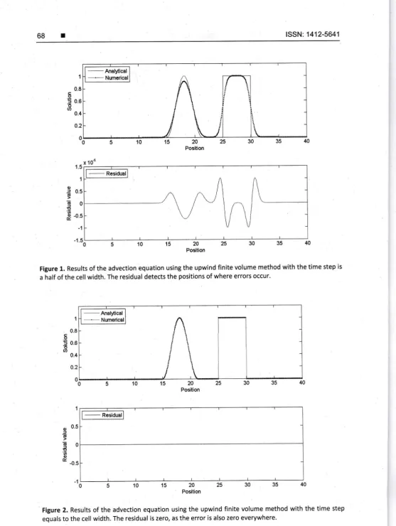
Figure 1. Results of the advection equation using the upwind finite volume method with the time step is

a half of the cell width. The residual detects the positions of where errors occur.

-

Residual

20 Position

Figure 2. Results of the advection equation using the upwind finite volume method with the time step

equals to the cell width. The residual iS zero, as the error is also zero everywhere'

30 25

't5

10

15

2A

25 Position

1

,

0.5

a

6

Eo

!,_'6 o

*

-0.5

-1

30 15

10

lledlaTeknika

ISSN: 1412-5641 69

810

x 1o-17

Residual

10 20 30 4U 5U 60 70 B0 90

180 [image:9.545.27.503.24.364.2] [image:9.545.47.516.401.713.2]

Position

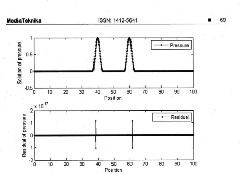
Figure 3. Pressure solution of the acoustics equations obtained using the Lax-Friedrichs finite volume method with the time step equals to the cell width, As the numerical solution is exact, the residual is

zero everywhere up to the machine precision. The magnitude of the residual is in the scale of 2.Oe-17 .

1 OT

u,

E

o.E o-o

Eo

=

c, m -tl.5 2 1 (lJ U' o o, L EL o

E

=

vt oJ E >1 .=_o g o} c, L .E

E

t/l

-(J E

E

(f

E

=

=

art o} E

40 5U

E0

Position

*Velocity

10u g0 BB 70 30 20 1 8.5 0 -0.5 -1 1 0.5 0 -0.5

01u

-d

x10'

40 50

E0

Fosition 1Uu 90 Eu 70 30 2E _1t

B 10 2B

30 4U 50 6U 78 BB

90 100

Position

Figure 4. Velocity solution of the acoustics equations found using the Lax-Friedrichs finite volume method with the time step equals to a half of the cell width. The residual finds the places where large

errors occur. The magnitude of the residual is in the scale of

l.0e-4.

70 ISSN: 1412-5641

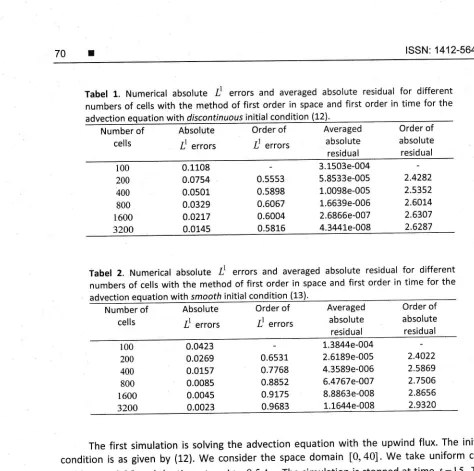
Tabel 1. Numerical absolute -C

"rrorr

and averaged absolute residual

for

different

numbers of cells with the method of first order in space and first order in time for the advection equation with drscontinuous _lnllel lenqlllen-ll?L

Number of

cells

Absolute

I

etrort

Order of

/

etrort

Averaged

absolute

residual

Order of absolute residual 100 200 400 800 1600 3200 0.1108 o.o754 0.0501 0.0329 0.02L7 0.0145 0.55s3 0.5898 0.6067 0.5004 0.5816 3.1503e-004 5.8533e-005 1.0098e-005 1.6639e-005 2.6866e-007 4.3441e-008 2.4282 2.5352 2.6014 2.6307 2.6287

Tabel 2. Numerical absolute -C errors and averaged absolute residual

for

different numbers of cells with the method of first order in space and first order in time for the advection equation with srnooth initial condition (13

Number of

cells

Absolute

-C

"rrort

Order of

/

etrott

Averaged

absolute

residual

Order of absolute residual 100 200 400 800 1600 3200 o.0423 0.0269 0.0157 0.008s 0.0045 0.0023 0.6531 0.7768 0.8852 0.9175 0.9683 1.3844e-004 2.6189e-005 4.3589e-006 6.4767e-007 8.8863e-008 1.1644e-008

z.iozz

2.s869 2.7506 2.8656 2.9320

The first simulation is solving the advection equation

with the

upwind flux. The initial

condition is as given by (12). We consider

the

space domain [0,

40].

We take uniform

cell-width

Ax = 0.05 and the time step A/ = 0.5 Ax . The simulation is stopped at

time

/

:

15 . The

analytical solution of this problem can be found from the work

of

LeVeque [5]. We find that

the largest errors occur at around discontinuities, as shown in Figure 1. ln Figure 1 we can also

observe that

the

residual values are

at

around discontinuities. This means that

the

residual concludes the same behaviour as the error.

ln

the

second simulation, we modify the time step of the first one' Now we take the

time step

to

be Af = Ax. Based on the characteristics method, the finite volume method with

the upwind flux formulation results in the exact solution. lndeed, we find the exact solution.

That is,

our

numerical solution matches exactly

with

the

analytical solution, as plotted in

Figure 2. As shown in Figure 2, we also observe that the residual values are zero everywhere.

This means that the residual behaves the same as the error.

The

third

simulation is about solving

the

acoustics equations. We consider

the

initial

condition (14)-(15).We consider

the

space

domain [0,100]. We take

uniform cell-width

Ax:0.1

and the time step

N =

Lx. We use the finite volume method with the Lax-Friedrichs

flux.

Based

on

the

characteristics theory

[5],

the

method results

in the

exact (analytical)

solution. However, we do not know the explicit form of the analytical solution. This is a good

test case if the residual for:mula can give the correct indication of the exact solution- At time

t=lO,the

simulation results are given in Figure 3. ln this figure there are two waves, that is,

one moves to the left and one moves to the right. The residual values are below the machine

precision (less

than 2xl0"r7l,

as shown in Figure 3. This means that our numerical solution is

actually the exact solution up to the machine precision.

[image:10.582.29.503.21.492.2]

MediaTeknika ISSN: 1412-5641

The fourth simulation is similar to the third one, but in this fourth simulation we change

the time step

to

A/ = 0.5

Ar.

Of course we shall not obtain the exact solution in this case. The

point of this simulation is

to

make sure that the residual can still detect where the positions have errors in

the

numerical solution. As shown

in

Figure 4,

the

residual indicates

that

the

largest errors occur at positions around large wave amplitudes. The error gets larger as time

evolves. This is because the amplitudes of waves, both moving to the left and right, dampen.

To complete our work, we investigate

the

behaviour

of the

residual as

the

grids are

refined. Firstly we consider the advection equation with initial condition (12) solved using the upwind finite volume method

with

&

= 0.5 Ax. The order of accuracy (order of error) is about

0.6, whereas

the

order

of the

residual is

about

2.6

,

as recorded in Table 1. Secondly we

consider

the

advection equation

with

initial

condition (13) solved using

the

upwind finite

volume method

with

A/ = 0.5 Ax, the same time step value as before. The order of accuracy

(order

of

error) is

about

1, whereas

the

order

of

the

residual is

about

3,

as recorded in Table 2. The order of error is larger for Table 2 than for Table 1, because of the difference in

their

initial conditions. The smoother

the

solution gives

the

larger

the

order

of

error. This

phenomena is also reflected in the residual results, shown in Tables 1 and 2.

4. Conclusion

Weak local residual has been shown

to

be

powerful

in

checking

the

accuracy of

numerical solutions where the exact solutions are

not

known. The behaviour of the residual

mimics that of the error. These results may help in the construction of smoothness indicator or

discontinuity detector

of

numerical solutions. Regions

of

where

numerical solutions are

accurate and

not

accurate can be identified using

a

smoothness indicator

or

discontinuity

detector.

References

11] Constantln LA, Kurganov A. Adaptive central-upwind schemes for hyperbolic systems of conservation laws. ln

F. Asakura et al., eds., Hyperbolic Problems: Theory, Numerics, and Applicotions, Vol. 1, pages 95-103. Yokohama Publishers, Yokohama, 2006.

t2l

Mungkasi S, Li Z, Roberts SG. Weak local residuals as smoothness indicators for the shallow water equations. Applied Mothemotics Letters. 2014; 30: 51-55.

t3J Dewar J, Kurganov A, Leopold M. Pressure-based adaption indicator for compressible Euler equations. Numericol Methods _for Portiol Differentiot Equotions.2015; 31: t84q-1874.

t4]

Mungkasi S, Roberts SG. Well-balanced computations of weak local residuals for the shallow water equations,

ANZTAM Journol. 2Ot5; 55: C72*C!47 .

tsl

LeVeque RJ. Finite-volume methods _for hyperbolic problems. Cambridge: Cambridge University Press. 2004.

71

Weak Local Residual in Relation to the Accuracy..., Sudi Mungkasi