Design Of Fuzzy Controllers
Jan Jantzen
[email protected]
:
1$EVWUDFW
Design of a fuzzy controller requires more design decisions than usual, for example regarding rule base, inference engine, defuzzification, and data pre- and post processing. This tutorial paper identifies and describes the design choices related to single-loop fuzzy control, based on an international standard which is underway. The paper contains also a design approach, which uses a PID controller as a starting point. A design engineer can view the paper as an introduction to fuzzy controller design.
&RQWHQWV
,QWURGXFWLRQ
6WUXFWXUH RI D IX]]\ FRQWUROOHU
2.1 Preprocessing 6
2.2 Fuzzification 7
2.3 Rule Base 7
2.4 Inference Engine 13
2.5 Defuzzification 15
2.6 Postprocessing 16
7DEOH %DVHG &RQWUROOHU
,QSXW2XWSXW 0DSSLQJ
7DNDJL6XJHQR 7\SH &RQWUROOHU
6XPPDU\
$ $GGLWLYH 5XOH %DVH
Technical University of Denmark, Department of Automation, Bldg 326, DK-2800 Lyngby, DENMARK.
,QWURGXFWLRQ
While it is relatively easy to design a PID controller, the inclusion of fuzzy rules creates many extra design problems, and although many introductory textbooks explain fuzzy con-trol, there are few general guidelines for setting the parameters of a simple fuzzy controller. The approach here is based on a three step design procedure, that builds on PID control:
1. Start with a PID controller.
2. Insert an equivalent, linear fuzzy controller. 3. Make it gradually nonlinear.
Guidelines related to the different components of the fuzzy controller will be intro-duced shortly. In the next three sections three simple realisations of fuzzy controllers are described: a table-based controller, an input-output mapping and a Takagi-Sugeno type controller. A short section summarises the main design choices in a simple fuzzy controller by introducing a check list. The terminology is based on an international standard which is underway (IEC, 1996).
Fuzzy controllers are used to control consumer products, such as washing machines, video cameras, and rice cookers, as well as industrial processes, such as cement kilns, underground trains, and robots. Fuzzy control is a control method based on fuzzy logic. Just as fuzzy logic can be described simply as ’’computing with words rather than numbers’’, fuzzy control can be described simply as ’’control with sentences rather than equations’’. A fuzzy controller can include empirical rules, and that is especially useful in operator controlled plants.
Take for instance a typical fuzzy controller
1. If error is Neg and change in error is Neg then output is NB
2. If error is Neg and change in error is Zero then output is NM (1)
The collection of rules is called aUXOH EDVH. The rules are in the familiar if-then format, and formally the if-side is called theFRQGLWLRQand the then-side is called theFRQFOXVLRQ(more often, perhaps, the pair is calledDQWHFHGHQW -FRQVHTXHQW orSUHPLVH -FRQFOXVLRQ). The input value ’’Neg’’ is aOLQJXLVWLF WHUPshort for the word1HJDWLYHthe output value ’’NB’’ stands for1HJDWLYH %LJand ’’NM’’ for1HJDWLYH 0HGLXP. The computer is able to execute the rules and compute a control signal depending on the measured inputsHUURUandFKDQJH LQ HUURU.
Deviations Actions Outputs Ref
Controller
End-user
Inference engine Rule base
Process
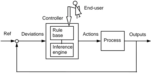
Figure 1: Direct control.
to isolate the control strategy in a rule base for operator controlled systems.
Fuzzy controllers are being used in various control schemes (IEC, 1996). The most obvious one isGLUHFW FRQWURO, where the fuzzy controller is in the forward path in a feedback control system (Fig. 1). The process output is compared with a reference, and if there is a deviation, the controller takes action according to the control strategy. In the figure, the arrows may be understood as hyper-arrows containing several signals at a time for multi-loop control. The sub-components in the figure will be explained shortly. The controller is here a fuzzy controller, and it replaces a conventional controller, say, a3,' (proportional-integral-derivative) controller.
InIHHGIRUZDUG FRQWURO (Fig. 2) a measurable disturbance is being compensated. It re-quires a good model, but if a mathematical model is difficult or expensive to obtain, a fuzzy model may be useful. Figure 2 shows a controller and the fuzzy compensator, the process and the feedback loop are omitted for clarity. The scheme, disregarding the disturbance in-put, can be viewed as a collaboration of linear and nonlinear control actions; the controller C may be a linear PID controller, while the fuzzy controller F is a supplementary nonlinear controller
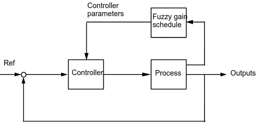
Fuzzy rules are also used to correct tuning parameters inSDUDPHWHU DGDSWLYH FRQWURO schemes (Fig. 3). If a nonlinear plant changes operating point, it may be possible to change the parameters of the controller according to each operating point. This is called JDLQ VFKHGXOLQJ since it was originally used to change process gains. A gain scheduling controller contains a linear controller whose parameters are changed as a function of the operating point in a preprogrammed way. It requires thorough knowledge of the plant, but it is often a good way to compensate for nonlinearities and parameter variations. Sensor measurements are used asVFKHGXOLQJ YDULDEOHV that govern the change of the controller parameters, often by means of a table look-up.
+ + Sum F
Fuzzy compensator
C
Controller
u Deviation
Disturbance
Figure 2: Feedforward control.
Outputs Ref
Controller Process
Fuzzy gain schedule Controller
parameters
for example by checking that all eigenvalues are in the left half of the complex plane. For nonlinear systems, and fuzzy systems are most often nonlinear, the stability concept is more complex. A nonlinear system is said to beDV\PSWRWLFDOO\ VWDEOH if, when it starts close to an equilibrium, it will converge to it. Even if it just stays close to the equilibrium, without converging to it, it is said to beVWDEOH (in the sense of Lyapunov). To check conditions for stability is much more difficult with nonlinear systems, partly because the system behav-iour is also influenced by the signalDPSOLWXGHVapart from theIUHTXHQFLHV. The literature is somewhat theoretical and interested readers are referred to Driankov, Hellendoorn & Reinfrank (1993) or Passino & Yurkovich (1998). They report on four methods (Lyapunov functions, Popov, circle, and conicity), and they give several references to scientific papers. It is characteristic, however, that the methods give rather conservative results, which trans-late into unrealistically small magnitudes of the gain factors in order to guarantee stability. Another possibility is to approximate the fuzzy controller with a linear controller, and then apply the conventional linear analysis and design procedures on the approximation. It seems likely that the stability margins of the nonlinear system would be close in some sense to the stability margins of the linear approximation depending on how close the approxi-mation is. This paper shows how to build such a linear approxiapproxi-mation, but the theoretical background is still unexplored.
There are at least four main sources for finding control rules (Takagi & Sugeno in Lee, 1990).
([SHUW H[SHULHQFH DQG FRQWURO HQJLQHHULQJ NQRZOHGJH One classical example is the operator’s handbook for a cement kiln (Holmblad & Ostergaard, 1982). The most com-mon approach to establishing such a collection of rules of thumb, is to question experts or operators using a carefully organised questionnaire.
%DVHG RQ WKH RSHUDWRU¶V FRQWURO DFWLRQV FuzzyLIWKHQ rules can be deduced from ob-servations of an operator’s control actions or a log book. The rules express input-output relationships.
%DVHG RQ D IX]]\ PRGHO RI WKH SURFHVV A linguistic rule base may be viewed as an inverse model of the controlled process. Thus the fuzzy control rules might be obtained by inverting a fuzzy model of the process. This method is restricted to relatively low order systems, but it provides an explicit solution assuming that fuzzy models of the open and closed loop systems are available (Braae & Rutherford in Lee, 1990). Another approach isIX]]\ LGHQWLILFDWLRQ (Tong; Takagi & Sugeno; Sugeno – all in Lee, 1990; Pedrycz, 1993) or fuzzy model-based control (see later).
%DVHG RQ OHDUQLQJ The self-organising controller is an example of a controller that finds the rules itself. Neural networks is another possibility.
There is no design procedure in fuzzy control such as root-locus design, frequency re-sponse design, pole placement design, or stability margins, because the rules are often non-linear. Therefore we will settle for describing the basic components and functions of fuzzy controllers, in order to recognise and understand the various options in commercial soft-ware packages for fuzzy controller design.
1995), but there is no agreement on the terminology, which is confusing. There are efforts, however, to standardise the terminology, and the following makes use of a draft of a stan-dard from the International Electrotechnical Committee (IEC, 1996). Throughout, letters denoting matrices are in bold upper case, for example$; vectors are in bold lower case, for example[; scalars are in italics, for exampleQ; and operations are in bold, for example PLQ.
6WUXFWXUH RI D IX]]\ FRQWUROOHU
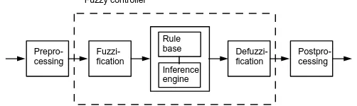
There are specific components characteristic of a fuzzy controller to support a design pro-cedure. In the block diagram in Fig. 4, the controller is between a preprocessing block and a post-processing block. The following explains the diagram block by block.
Fuzzy controller
Inference engine Rule
base Defuzzi-fication
Postpro-cessing
Fuzzi-fication
Prepro-cessing
Figure 4: Blocks of a fuzzy controller.
3UHSURFHVVLQJ
The inputs are most often hard orFULVS measurements from some measuring equipment, rather than linguistic. A preprocessor, the first block in Fig. 4, conditions the measurements before they enter the controller. Examples of preprocessing are:
Quantisation in connection with sampling or rounding to integers; normalisation or scaling onto a particular, standard range; filtering in order to remove noise;
averaging to obtain long term or short term tendencies;
a combination of several measurements to obtain key indicators; and differentiation and integration or their discrete equivalences.
ATXDQWLVHUis necessary to convert the incoming values in order to find the best level in a discreteXQLYHUVH. Assume, for instance, that the variableHUURU has the value 4.5, but the universe isX @ +8>7> = = = >3> = = = >7>8,. The quantiser rounds to 5 to fit it to the nearest level. Quantisation is a means to reduce data, but if the quantisation is too coarse the controller may oscillate around the reference or even become unstable.
-5 0 5 -100
0 100
input
s
c
a
led input
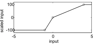
Figure 5: Example of nonlinear scaling of an input measurement.
to enter three typical numbers for a small, medium and large measurement respectively (Holmblad & Østergaard, 1982). They become break-points on a curve that scales the incoming measurements (circled in the figure). The overall effect can be interpreted as a distortion of the primary fuzzy sets. It can be confusing with both scaling and gain factors in a controller, and it makes tuning difficult.
When the input to the controller isHUURU, the control strategy is a static mapping between input and control signal. A dynamic controller would have additional inputs, for example derivatives, integrals, or previous values of measurements backwards in time. These are created in the preprocessor thus making the controller multi-dimensional, which requires many rules and makes it more difficult to design.
The preprocessor then passes the data on to the controller.
)X]]LILFDWLRQ
The first block inside the controller isIX]]LILFDWLRQ, which converts each piece of input data to degrees of membership by a lookup in one or several membership functions. The fuzzification block thus matches the input data with the conditions of the rules to determine how well the condition of each rule matches that particular input instance. There is a degree of membership for each linguistic term that applies to that input variable.
5XOH %DVH
The rules may use several variables both in the condition and the conclusion of the rules. The controllers can therefore be applied to both multi-input-multi-output (MIMO) problems and single-input-single-output (SISO) problems. The typical SISO problem is to regulate a control signal based on an error signal. The controller may actually need both theHUURU, theFKDQJH LQ HUURU, and theDFFXPXODWHG HUURU as inputs, but we will call it single-loop control, because in principle all three are formed from the error measurement. To simplify, this section assumes that the control objective is to regulate some process output around a prescribed setpoint or reference. The presentation is thus limited to single-loop control.
end-user in a format similar to the one below,
1. If error is Neg and change in error is Neg then output is NB 2. If error is Neg and change in error is Zero then output is NM 3. If error is Neg and change in error is Pos then output is Zero 4. If error is Zero and change in error is Neg then output is NM
5. If error is Zero and change in error is Zero then output is Zero (2) 6. If error is Zero and change in error is Pos then output is PM
7. If error is Pos and change in error is Neg then output is Zero 8. If error is Pos and change in error is Zero then output is PM 9. If error is Pos and change in error is Pos then output is PB
The names=HUR,3RV,1HJ are labels of fuzzy sets as well as 1%,10,3% and30 (negative big, negative medium, positive big, and positive medium respectively). The same set of rules could be presented in aUHODWLRQDO format, a more compact representation.
Error Change in error Output
Neg Pos Zero
Neg Zero NM
Neg Neg NB
Zero Pos PM
Zero Zero Zero
Zero Neg NM
Pos Pos PB
Pos Zero PM
Pos Neg Zero
(3)
The top row is the heading, with the names of the variables. It is understood that the two leftmost columns are inputs, the rightmost is the output, and each row represents a rule. This format is perhaps better suited for an experienced user who wants to get an overview of the rule base quickly. The relational format is certainly suited for storing in a relational database. It should be emphasised, though, that the relational format implicitly assumes that the connective between the inputs is always logicalDQGor logicalRUfor that matter as long as it is the same operation for all rulesand not a mixture of connectives. Incidentally, a fuzzy rule with anRUcombination of terms can be converted into an equivalent DQG combination of terms using laws of logic (DeMorgan’s laws among others). A third format is the tabular linguistic format.
Change in error Neg Zero Pos
Neg NB NM Zero
Error Zero NM Zero PM
Pos Zero PM PB
(4)
rule, and this format is useful for checking completeness. When the input variables areHUURU andFKDQJH LQ HUURU, as they are here, that format is also called aOLQJXLVWLF SKDVH SODQH. In case there areq A5input variables involved, the table grows to anq-dimensional array; rather user-XQfriendly.
To accommodate several outputs, a nested arrangement is conceivable. A rule with several outputs could also be broken down into several rules with one output.
Lastly, a graphical format which shows the fuzzy membership curves is also possible (Fig. 7). This graphical user-interface can display the inference process better than the other formats, but takes more space on a monitor.
&RQQHFWLYHV In mathematics, sentences are connected with the wordsDQG,RU,LIWKHQ (orLPSOLHV, andLI DQG RQO\ LI, or modifications with the wordQRW. These five are called FRQQHFWLYHV. It also makes a difference how the connectives are implemented. The most prominent is probably multiplication for fuzzyDQGinstead of minimum. So far most of the examples have only containedDQGoperations, but a rule like ‘‘If error is very neg and not zero or change in error is zero then ...’’ is also possible.
The connectivesDQGandRUare always defined in pairs, for example, D DQG E@PLQ+D>E, minimum
D RU E@PD[+D>E, maximum or
D DQG E@DE algebraic product
D RU [email protected] algebraic or probabilistic sum
(5)
There are other examples (e.g., Zimmermann, 1991,6465,, but they are more com-plex.
0RGLILHUV A linguisticPRGLILHU, is an operation that modifies the meaning of a term. For example, in the sentence ‘‘very close to 0’’, the wordYHU\modifies&ORVH WR which is a fuzzy set. A modifier is thus an operation on a fuzzy set. The modifierYHU\can be defined as squaring the subsequent membership function, that is
YHU\ D@D5 (6)
Some examples of other modifiers are H[WUHPHO\ D@D6 VOLJKWO\ D@D46
VRPHZKDW D@PRUHRUOHVV D DQG QRW VOLJKWO\ D
A whole family of modifiers is generated byDs wheresis any power between zero and infinity. Withs@4the modifier could be namedH[DFWO\, because it would suppress all memberships lower than 1.0.
8QLYHUVHV Elements of a fuzzy set are taken from aXQLYHUVH RI GLVFRXUVHor justXQLYHUVH. The universe contains all elements that can come into consideration. Before designing the membership functions it is necessary to consider the universes for the inputs and outputs. Take for example the rule
Naturally, the membership functions for1HJ and3RV must be defined for all possible values ofHUURUandFKDQJH LQ HUURUand a standard universe may be convenient.
Another consideration is whether the input membership functions should be continuous or discrete. A continuous membership function is defined on a continuous universe by means of parameters. A discrete membership function is defined in terms of a vector with a finite number of elements. In the latter case it is necessary to specify the range of the universe and the value at each point. The choice between fine and coarse resolution is a trade off between accuracy, speed and space demands. The quantiser takes time to execute, and if this time is too precious, continuous membership functions will make the quantiser obsolete.
([DPSOH VWDQGDUG XQLYHUVHV 0DQ\ DXWKRUV DQG VHYHUDO FRPPHUFLDO FRQWUROOHUV XVH VWDQGDUG XQLYHUVHV
7KH )/ 6PLGWK FRQWUROOHU IRU LQVWDQFH XVHV WKH UHDO QXPEHU LQWHUYDO ^4>4` $XWKRUV RI WKH HDUOLHU SDSHUV RQ IX]]\ FRQWURO XVHG WKH LQWHJHUV LQ^9>9`
$QRWKHU SRVVLELOLW\ LV WKH LQWHUYDO ^433>433` FRUUHVSRQGLQJ WR SHUFHQWDJHV RI IXOO VFDOH
<HW DQRWKHU LV WKH LQWHJHU UDQJH ^3>73<8` FRUUHVSRQGLQJ WR WKH RXWSXW IURP D ELW DQDORJ WR GLJLWDO FRQYHUWHU
$ YDULDQW LV^537:>537;`>ZKHUH WKH LQWHUYDO LV VKLIWHG LQ RUGHU WR DFFRPPRGDWH QHJ DWLYH QXPEHUV
7KH FKRLFH RI GDWDW\SHV PD\ JRYHUQ WKH FKRLFH RI XQLYHUVH )RU H[DPSOH WKH YROWDJH UDQJH^8>8`FRXOG EH UHSUHVHQWHG DV DQ LQWHJHU UDQJH^83>83` RU DV D IORDWLQJ SRLQW UDQJH^8=3>8=3` D VLJQHG E\WH GDWDW\SH KDV DQ DOORZDEOH LQWHJHU UDQJH^45;>45:`
A way to exploit the range of the universes better is scaling. If a controller input mostly uses just one term, the scaling factor can be turned up such that the whole range is used. An advantage is that this allows a standard universe and it eliminates the need for adding more terms.
0HPEHUVKLS IXQFWLRQV Every element in the universe of discourse is a member of a fuzzy set to some grade, maybe even zero. The grade of membership for all its members describes a fuzzy set, such as1HJ. In fuzzy sets elements are assigned aJUDGH RI PHPEHU VKLS, such that the transition from membership to non-membership is gradual rather than abrupt. The set of elements that have a non-zero membership is called theVXSSRUW of the fuzzy set. The function that ties a number to each element{of the universe is called the PHPEHUVKLS IXQFWLRQ+{,.
The designer is inevitably faced with the question of how to build the term sets. There are two specific questions to consider: (i) How does one determine the shape of the sets? and (ii) How many sets are necessary and sufficient? For example, theHUURUin the position controller uses the family of terms1HJ,=HUR, and3RV. According to fuzzy set theory the choice of the shape and width is subjective, but a few rules of thumb apply.
0 0.5 1
(a) (d) (g) (j)
0 0.5 1
(b) (e) (h) (k)
-1000 0 100
0.5 1
(c)
-100 0 100
(f)
-100 0 100
(i)
-100 0 100
(l)
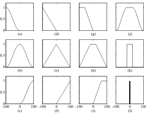
Figure 6: Examples of membership functions. Read from top to bottom, left to right: (a) sfunction, (b)function, (c) zfunction, (d-f) triangular versions, (g-i) trapezoidal versions, (j) flatfunction, (k) rectangle, (l) singleton.
A certain amount of overlap is desirable; otherwise the controller may run into poorly defined states, where it does not return a well defined output.
A preliminary answer to questions (i) and (ii) is that the necessary and sufficient number of sets in a family depends on the width of the sets, and vice versa. A solution could be to ask the process operators to enter their personal preferences for the membership curves; but operators also find it difficult to settle on particular curves.
The manual for the TILShell product recommends the following (Hill, Horstkotte & Teichrow, 1990).
6WDUW ZLWK WULDQJXODU VHWV All membership functions for a particular input or output should be symmetrical triangles of the same width. The leftmost and the rightmost should be shouldered ramps.
7KH RYHUODS VKRXOG EH DW OHDVW The widths should initially be chosen so that each value of the universe is a member of at least two sets, except possibly for elements at the extreme ends. If, on the other hand, there is a gap between two sets no rules fire for values in the gap. Consequently the controller function is not defined.
Strictly speaking, a fuzzy setDis a collection of ordered pairs
D@i+{> +{,,j (7) Item{belongs to the universe and+{,is its grade of membership inD. A single pair +{> +{,,is a fuzzyVLQJOHWRQ;VLQJOHWRQ RXWSXW means replacing the fuzzy sets in the con-clusion by numbers (scalars). For example
1. If error is Pos then output is43volts 2. If error is Zero then output is3volts 3. If error is Neg then output is 43volts There are at least three advantages to this:
The computations are simpler;
it is possible to drive the control signal to its extreme values; and it may actually be a more intuitive way to write rules.
The scalar can be a fuzzy set with the singleton placed in a proper position. For ex-ample43YROWV, would be equivalent to the fuzzy set+3>3>3>3>4,defined on the universe +43>8>3>8>43,YROWV.
([DPSOH PHPEHUVKLS IXQFWLRQV )X]]\ FRQWUROOHUV XVH D YDULHW\ RI PHPEHUVKLS IXQF WLRQV $ FRPPRQ H[DPSOH RI D IXQFWLRQ WKDW SURGXFHV D EHOO FXUYH LV EDVHG RQ WKH H[SRQHQ WLDO IXQFWLRQ
7KLV LV D VWDQGDUG *DXVVLDQ FXUYH ZLWK D PD[LPXP YDOXH RI4{LV WKH LQGHSHQGHQW YDULDEOH RQ WKH XQLYHUVH{3LV WKH SRVLWLRQ RI WKH SHDN UHODWLYH WR WKH XQLYHUVH DQGLV WKH VWDQGDUG GHYLDWLRQ $QRWKHU GHILQLWLRQ ZKLFK GRHV QRW XVH WKH H[SRQHQWLDO LV
+{, @
7KH IO VplgwkFRQWUROOHU XVHV WKH HTXDWLRQ
+{, @ 4h{s
7KH H[WUD SDUDPHWHUdFRQWUROV WKH JUDGLHQW RI WKH VORSLQJ VLGHV ,W LV DOVR SRVVLEOH WR XVH RWKHU IXQFWLRQV IRU H[DPSOH WKH vljprlgNQRZQ IURP QHXUDO QHWZRUNV
$frvlqh IXQFWLRQ FDQ EH XVHG WR JHQHUDWH D YDULHW\ RI PHPEHUVKLS IXQFWLRQV 7KH
v0fxuyhFDQ EH LPSOHPHQWHG DV
Figure 7: Graphical construction of the control signal in a fuzzy PD controler (generated in the Matlab Fuzzy Logic Toolbox).
WLRQ
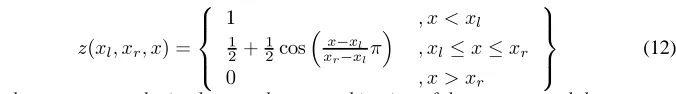
}+{o> {u> {, @ ; A ? A =
4 > { ? {o 4
5.45frv
{{o {u{o
> {o{{u
3 > { A {u
< A @ A
> (12)
7KHQ WKH0fxuyhFDQ EH LPSOHPHQWHG DV D FRPELQDWLRQ RI WKH v0fxuyhDQG WKH }0fxuyh VXFK WKDW WKH SHDN LV IODW RYHU WKH LQWHUYDO^{5> {6`
+{4> {5> {6> {7> {, @ plq+v+{4> {5> {,> }+{6> {7> {,, (13)
,QIHUHQFH (QJLQH
chart. For each rule, the inference engine looks up the membership values in the condition of the rule.
$JJUHJDWLRQ TheDJJUHJDWLRQ operation is used when calculating theGHJUHH RI IXOILOO PHQW orILULQJ VWUHQJWK n of the condition of a rulen. A rule, say rule 1, will generate a fuzzy membership valueh4coming from theHUURUand a membership valuefh4coming from theFKDQJH LQ HUURU measurement. The aggregation is their combination,
h4DQGfh4 (14)
Similarly for the other rules. Aggregation is equivalent to fuzzification, when there is only one input to the controller. Aggregation is sometimes also calledIXOILOPHQW of the rule or ILULQJ VWUHQJWK.
$FWLYDWLRQ TheDFWLYDWLRQof a rule is the deduction of the conclusion, possibly reduced by its firing strength. Thickened lines in the third column indicate the firing strength of each rule. Only the thickened part of the singletons are activated, andPLQor product (*) is used as theDFWLYDWLRQ RSHUDWRU. It makes no difference in this case, since the output membership functions are singletons, but in the general case ofv> >and}functions in the third column, the multiplication scales the membership curves, thus preserving the initial shape, rather than clipping them as thePLQoperation does. Both methods work well in general, although the multiplication results in a slightly smoother control signal. In Fig. 7, only rules four and five are active.
A rulencan be weighted a priori by a weighting factor$n 5^3>4`, which is itsGHJUHH RI FRQILGHQFHIn that case the firing strength is modified to
n @$nn= (15) The degree of confidence is determined by the designer, or a learning program trying to adapt the rules to some input-output relationship.
$FFXPXODWLRQ All activated conclusions areDFFXPXODWHG, using the PD[operation, to the final graph on the bottom right (Fig. 7). Alternatively,VXPaccumulation counts overlapping areas more than once (Fig. 8). Singleton output (Fig. 7) andVXPaccumulation results in the simple output
4v4.5v5.= = =.qvq (16) The alpha’s are the firing strengths from theqrules andv4...vqare the output singletons. Since this can be computed as a vector product, this type of inference is relatively fast in a matrix oriented language.
'HIX]]LILFDWLRQ
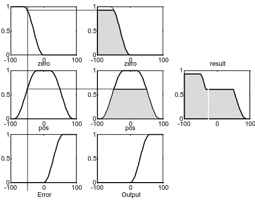
The resulting fuzzy set (Fig. 7, bottom right; Fig. 8, extreme right) must be converted to a number that can be sent to the process as a control signal. This operation is called GHIX]]LILFDWLRQ, and in Fig. 8 the{-coordinate marked by a white, vertical dividing line becomes the control signal. The resulting fuzzy set is thus defuzzified into a crisp control signal. There are several defuzzification methods.
&HQWUH RI JUDYLW\ &2* The crisp output valuex(white line in Fig. 8) is the abscissa under the centre of gravity of the fuzzy set,
x@ membership function. The expression can be interpreted as the weighted average of the elements in the support set. For the continuous case, replace the summations by integrals. It is a much used method although its computational complexity is relatively high. This method is also calledFHQWURLG RI DUHD.
&HQWUH RI JUDYLW\ PHWKRG IRU VLQJOHWRQV &2*6 If the membership functions of the conclusions are singletons (Fig. 7), the output value is
x@ S
l+vl,vl S
l+vl, (18)
Herevlis the position of singletonlin the universe, and+vl,is equal to the firing strength
lof rulel. This method has a relatively good computational complexity, andxis differ-entiable with respect to the singletonsvl, which is useful in neurofuzzy systems.
%LVHFWRU RI DUHD %2$ This method picks the abscissa of the vertical line that divides the area under the curve in two equal halves. In the continuous case,
x@
Here{is the running point in the universe,+{,is its membership,P lqis the leftmost value of the universe, andP d{is the rightmost value. Its computational complexity is relatively high, and it can be ambiguous. For example, if the fuzzy set consists of two singletons any point between the two would divide the area in two halves; consequently it is safer to say that in the discrete case, BOA is not defined.
0HDQ RI PD[LPD 020 An intuitive approach is to choose the point with the strongest possibility, i.e. maximal membership. It may happen, though, that several such points exist, and a common practice is to take thePHDQ RI PD[LPD(MOM). This method disregards the shape of the fuzzy set, but the computational complexity is relatively good.
/HIWPRVW PD[LPXP /0 DQG ULJKWPRVW PD[LPXP 50 Another possibility is to
-1000 0 100
Figure 8: One input, one output rule base with non-singleton output sets.
it. The defuzzifier must then choose one or the other, not something in between. These methods are indifferent to the shape of the fuzzy set, but the computational complexity is relatively small.
3RVWSURFHVVLQJ
Output scaling is also relevant. In case the output is defined on a standard universe this must be scaled toHQJLQHHULQJ XQLWVfor instance, volts, meters, or tons per hour. An example is the scaling from the standard universe^4>4`to the physical units^43>43`volts.
The postprocessing block often contains an output gain that can be tuned, and sometimes also an integrator.
([DPSOH LQIHUHQFH +RZ LV WKH LQIHUHQFH LQ )LJ 8LPSOHPHQWHG XVLQJ GLVFUHWH IX]]\ VHWV"
%HKLQG WKH VFHQH DOO XQLYHUVHV ZHUH GLYLGHG LQWR534SRLQWV IURP433WR433 %XW IRU EUHYLW\ OHW XV MXVW XVH ILYH SRLQWV $VVXPH WKH XQLYHUVHX FRPPRQ WR DOO YDULDEOHV LV WKH YHFWRU
X@ 433 83 3 83 433
$frvlqh IXQFWLRQ FDQ EH XVHG WR JHQHUDWH D YDULHW\ RI PHPEHUVKLS IXQFWLRQV 7KH
ZKHUH{oLV WKH OHIW EUHDNSRLQW DQG{uLV WKH ULJKW EUHDNSRLQW 7KH }0fxuyhLV MXVW D UHIOHF
7KHQ WKH0fxuyhVHH IRU H[DPSOH )LJ6M FDQ EH LPSOHPHQWHG DV D FRPELQDWLRQ RI WKH
v0fxuyhDQG WKH }0fxuyh VXFK WKDW WKH SHDN LV IODW RYHU WKH LQWHUYDO^{5> {6`
+{4> {5> {6> {7> {, @ plq+v+{4> {5> {,> }+{6> {7> {,, (22) $ IDPLO\ RI WHUPV LV GHILQHG E\ PHDQV RI WKHIXQFWLRQ VXFK WKDW
QHJ@+433>433>93>43>X, @ 4 3=<8 3=38 3 3 ]HUR@+<3>53>53><3>X, @ 3 3=94 4 3=94 3 SRV@+43>93>433>433>X, @ 3 3 3=38 3=<8 4
$ERYH ZH LQVHUWHG WKH ZKROH YHFWRUXLQ SODFH RI WKH UXQQLQJ SRLQW { WKH UHVXOW LV WKXV
D YHFWRU 7KH ILJXUH DVVXPHV WKDW huuru@83WKH XQLW LV SHUFHQWDJHV RI IXOO UDQJH 7KLV FRUUHVSRQGV WR WKH VHFRQG SRVLWLRQ LQ WKH XQLYHUVH DQG WKH ILUVW UXOH FRQWULEXWHV ZLWK D PHPEHUVKLSQHJ+5, @ 3=<8 7KLV ILULQJ VWUHQJWK LV SURSDJDWHG WR WKH FRQFOXVLRQ VLGH RI WKH UXOH XVLQJPLQ VXFK WKDW WKH FRQWULEXWLRQ IURP WKLV UXOH LV
3=<8PLQ QHJ@ 3=<8 3=<8 3=38 3 3
7KH DFWLYDWLRQ RSHUDWLRQ ZDVPLQKHUH $SSO\ WKH VDPH SURFHGXUH WR WKH WZR UHPDLQLQJ
UXOHV DQG VWDFN DOO WKUHH FRQWULEXWLRQV RQ WRS RI HDFK RWKHU 3=<8 3=<8 3=38 3 3
3 3=94 3=94 3=94 3
3 3 3 3 3
7R ILQG WKH DFFXPXODWHG RXWSXW VHW SHUIRUP DPD[RSHUDWLRQ GRZQ HDFK FROXPQ 7KH
UHVXOW LV WKH YHFWRU
3=<8 3=<8 3=94 3=94 3 7KH fhqwuh ri judylw|PHWKRG \LHOGV
x @
ZKLFK LV WKH FRQWURO VLJQDO EHIRUH SRVWSURFHVVLQJ
7DEOH %DVHG &RQWUROOHU
between all input combinations and their corresponding outputs are arranged in a table. With two inputs and one output, the table is a two-dimensional look-up table. With three inputs the table becomes a three-dimensional array. The array implementation improves execution speed, as the run-time inference is reduced to a table look-up which is a lot faster, at least when the correct entry can be found without too much searching. Below is a small example of a look-up table corresponding to the rulebase (2) with the membership functions in Fig. 7,
change in error
-100 -50 0 50 100
-100 -200 -160 -100 -40 0
-50 -160 -121 -61 0 40
error 0 -100 -61 0 61 100
50 -40 0 61 121 160
100 0 40 100 160 200
(26)
A typical application area for the table based controller is where the inputs to the con-troller are theHUURU and theFKDQJH LQ HUURU. The controller can be embedded in a larger system, a car for instance, where the table is downloaded to a table look-up mechanism.
7DEOH UHJLRQV Referring to the look-up table (26), a negative value ofHUURU implies that the process output| is above the referenceUhi, because the error is computed as
huuru @ Uhi |. A positive value implies a process output below the reference. A negative value ofFKDQJH LQ HUURUmeans that the process output increases while a positive value means it decreases.
Certain regions in the table are especially interesting. The centre of the table corre-sponds to the case where theHUURUis zero, the process is on the reference. Furthermore, the FKDQJH LQ HUURUis zero here, so the process stays on the reference. This position is the sta-ble point where the process has settled on the reference. The anti-diagonal (orthogonal to the main diagonal) of the table is zero; those are all the pleasant states, where the process is either stable on the reference or approaching the reference. Should the process move away a little from the zero diagonal, due to noise or a disturbance, the controller will make small corrections to get it back. In case the process is far from the reference and also moving away from it, we are in the upper left and lower right corners. Here the controller calls for drastic changes.
The numerical values on the two sides of the zero diagonal do not have to be anti-symmetric; they can be any values, reflecting asymmetric control strategies. During a re-sponse with overshoot after a positive step in the reference, a plot of the point+HUURU>FKDQJH LQ HUURU,will follow a trajectory in the table which spirals clockwise from the lower left corner of the table towards the centre. It is similar to aSKDVH SODQHtrajectory, where a vari-able is plotted against its derivative. A clever designer may adjust the numbers manually during a tuning session to obtain a particular response.
be avoided withELOLQHDU LQWHUSRODWLRQ between the cells instead of rounding to the nearest point. In the case of a two-dimensional table, an errorHsatisfies the relationH4H
H5, whereH4andH5are the two neighbouring points. The change-in-errorFHwill like-wise satisfyFH4FHFH5. The resulting table value is then found by interpolating linearly in theHaxis direction between the first pairx4 @ +I+H4> FH4,> I+H5> FH4,, and the second pairx5@ +I+H4> FH5,> I+H5> FH5,,, and then in theFH-axis direction between the pair+x4> x5,.
q'LPHQVLRQDO 7DEOHV A three input controller has a three-dimensional look-up table. Assuming a resolution of, say, 13 points in each universe, the table holds 2197 elements. It would be a tremendous task to fill these in manually, but it is manageable with rules.
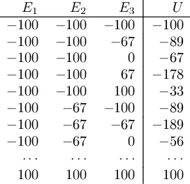
A three dimensional table can be represented as a two-dimensional table using a re-lational representation. Rearrange the table into three columns one for each of the three inputs+H4> H5> H6,and one for the output+X,>for example Table 1. Each input can take five values, and the table thus has888 @ 458rows. The table look-up is now a question of finding the right row, and picking the correspondingX value.
H4 H5 H6 X
433 433 433 433
433 433 9: ;<
433 433 3 9:
433 433 9: 4:;
433 433 433 66
433 9: 433 ;<
433 9: 9: 4;<
433 9: 3 89
433 433 433 433
Table 1: Equivalent of a 3D look-up table.
,QSXW2XWSXW 0DSSLQJ
Two inputs and one output results in a two dimensional table, which can be plotted as a surface for visual inspection. The relationship between one input and one output can be plotted as a graph. These plots are a design aid when selecting membership functions and constructing rules.
The shape of the surface can be controlled to a certain extent by manipulating the mem-bership functions. In order to see this clearly, we will use the one-input-one-output case (without loss of generality). The fuzzy proportional rule base
1. If error is Neg then output is Neg
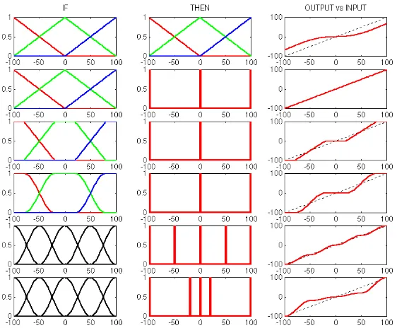
Figure 9: Input-output maps of proportional controllers. Each row is a controller.
3. If error is Pos then output is Pos
produced the six different mappings in Fig. 9. The rightmost column is the input-output mapping, and each row is a different controller. The controllers have the input families in theLI-column and the output families in theWKHQcolumn. The results depend on the choice of design parameters, which in this case are the following: the(SURGXFW) operation forDF WLYDWLRQbecause it is continuous, thePD[operation forDFFXPXODWLRQsince it corresponds to set union, andFHQWUH RI JUDYLW\ forGHIX]]LILFDWLRQ since it is continuous, unambiguous, and it degenerates to&2*6 in the case of singleton output. If there had been two or more inputs, theoperation forDQGwould be chosen since it is continuous. These choices are also necessary and sufficient for a linear mapping (appendix).
The following comments relate to the figure, row by row:
1. Triangular sets in both condition and conclusion result in a winding input-output map-ping. Compared to a linear controller (dotted line) the gain of the fuzzy controller varies. A slight problem with this controller is that it does not use the full output range; it is impossible to drive the output to 100%. Another problem is that the local gain is always equal or lower than the linear controller.
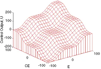
Figure 10: Example of a control surface.
input-output mapping is linear.
3. Flat input sets produce flat plateaus and large gains far away from the reference. This is similar to a deadzone with saturation. Increasing the width of the middle term results in a wider plateau around the reference. Less overlap between neighbouring sets will result in steeper slopes.
4. If the sharp corners cause problems, they are removed by introducing nonlinear input sets. The input-output relationship is now smooth.
5. Adding more sets only makes the mapping more bumpy.
6. On the other hand with more sets it is easier to stretch the reference plateau by moving the singletons about.
The experiment shows that depending on what the design specifications are, it is possi-ble to control, to a certain extent, the variation of the gain. Using singletons on the output side makes it easier. The results can easily be generalised to three dimensional surfaces. In all cases the activation operator was(product), the accumulation operator wasPD[, and the defuzzification method was&2* or&2*6 other operations may give slightly different results.
&RQWURO 6XUIDFH With two inputs and one output the input-output mapping is a surface. Figure 10 is a mesh plot of an example relationship betweenHUURU HandFKDQJH LQ HUURU
FHon the input side, and controller outputxon the output side. The plot results from a rule base with nine rules, and the surface is more or less bumpy. The horizontal plateaus are due to flat peaks on the input sets. The plateau around the origin implies a low sensitivity towards changes in eitherHUURUorFKDQJH LQ HUURUnear the reference. This is an advantage if noise sensitivity must be low when the process is near the reference. On the other hand, if the process is unstable in open loop it is difficult to keep the process on the reference, and it will be necessary to have a larger gain around the origin.
There are three sources of nonlinearity in a fuzzy controller.
scaling cause nonlinear transformations. The rules often express a nonlinear control strategy.
7KH LQIHUHQFH HQJLQH If the connectivesDQGandRUare implemented as for example PLQandPD[respectively, they are nonlinear.
7KH GHIX]]LILFDWLRQ. Several defuzzification methods are nonlinear.
It is possible to construct a rule base with a linear input-output mapping (Siler & Ying, 1989; Mizumoto, 1992; Qiao & Mizumoto; 1996). The following checklist summarises the general design choices for achieving a fuzzy rule base equivalent to a summation (details in the appendix):
Use triangular input sets that cross at@ 3=8> use the algebraic product (*) for theDQGconnective;
the rule base must be the completeDQGcombination (cartesian product) of all input families;
use output singletons, positions determined by the sum of the peak positions of the input sets;
use&2*6 defuzzification.
With these design choices the control surface degenerates to a diagonal plane (Fig. 11). A flexible fuzzy controller, that allows these choices, is two controllers in one so to speak. When linear, it has a transfer function and the usual methods regarding tuning and stability of the closed loop system apply.
Figure 11: Linear surface with trajectory of a transient response.
7DNDJL6XJHQR 7\SH &RQWUROOHU
0 50 100 0
50 100 150
(a)
outpu
t 1
2
0 50 100
0 0.5 1
(b)
m
em
ber
ship
Figure 12: Interpolation between two lines (a), and overlap of rules (b).
6XJHQRrule structure is
Ifi+h4is$4> h5is$5> = = = > hnis$n,then|@j+h4> h4= = =,
Herei is a logical function that connects the sentences forming the condition, | is the output, andjis a function of the inputs. A simple example is
If error is Zero and change in error is Zero then output|@f
wherefis a crisp constant. This is a]HURRUGHUmodel, and it is identical to singleton output rules. A slightly more complex rule is
If error is Zero and change in error is Zero then output
| @ dhuuru.e+fkdqjh lq huuru, .f
where d> eandfare all constants. This is a ILUVWRUGHU model. Inference with several rules proceeds as usual, with a firing strength associated with each rule, but each output is linearly dependent on the inputs. The output from each rule is a moving singleton, and the defuzzified output is the weighted average of the contributions from each rule. The controller interpolates between linear controllers; each controller is dominated by a rule, but there is a weighting depending on the overlap of the input membership functions. This is useful in a nonlinear control system, where each controller operates in a subspace of the operating envelope. One can say that the rules interpolate smoothly between the linear gains. Higher order models are also possible.
([DPSOH 6XJHQR 6XSSRVH ZH KDYH WZR UXOHV
,I HUURU LV /DUJH WKHQ RXWSXW LV /LQH ,I HUURU LV 6PDOO WKHQ RXWSXW LV /LQH
LQWHUSRODWH EHWZHHQ WKH WZR OLQHV LQ WKH UHJLRQ ZKHUH WKH PHPEHUVKLS IXQFWLRQV RYHUODS )LJ 12 2XWVLGH RI WKDW UHJLRQ WKH RXWSXW LV D OLQHDU IXQFWLRQ RI WKH huuru 7KLV W\SH RI PRGHO LV XVHG LQ QHXURIX]]\ V\VWHPV
In order to train a model to incorporate dynamics of a target system, the input is aug-mented with signals corresponding to past inputsxand outputs|. In the time discrete domain the output of the model|p>with superscriptpreferring to the model andsto the plant, is
|p+w. 4, @ei ^|s+w,> = = = > |s+wq. 4,>x+w,> = = = > x+wp. 4,` (28) Hereeirepresents the nonlinear input-output map of the model (i.e. the approximation of the target systemi). Notice that the input to the model includes the past values of the plant output|sand the plant inputx.
6XPPDU\
In a fuzzy controller the data passes through a preprocessing block, a controller, and a postprocessing block. Preprocessing consists of a linear or non-linear scaling as well as a quantisation in case the membership functions are discretised (vectors); if not, the mem-bership of the input can just be looked up in an appropriate function. When designing the rule base, the designer needs to consider the number of term sets, their shape, and their overlap. The rules themselves must be determined by the designer, unless more advanced means like self-organisation or neural networks are available. There is a choice between multiplication and minimum in the activation. There is also a choice regarding defuzzifi-cation;FHQWUH RI JUDYLW\ is probably most widely used. The postprocessing consists in a scaling of the output. In case the controller is incremental, postprocessing also includes an integration. The following is a checklist of design choices that have to be made:
5XOH EDVH UHODWHG FKRLFHV. Number of inputs and outputs, rules, universes, continuous
@discrete, the number of membership functions, their overlap and width, singleton output;
,QIHUHQFH HQJLQH UHODWHG FKRLFHV. Connectives, modifiers, activation operation, aggre-gation operation, and accumulation operation.
'HIX]]LILFDWLRQ PHWKRG. COG, COGS, BOA, MOM, LM, and RM.
3UH DQG SRVWSURFHVVLQJ. Scaling, gain factors, quantisation, and sampling time.
Some of these items must always be considered, others may not play a role in the par-ticular design.
The input-output mappings provide an intuitive insight which may not be relevant from a theoretical viewpoint, but in practice they are well worth using. The analysis represented by plots is limited, though, to three dimensions. Various input-output mappings can be obtained by changing the fuzzy membership functions, and the chapter shows how to obtain a linear mapping with only a few adjustments.
1. Tune a PID controller.
2. Replace it with a linear fuzzy controller. 3. Transfer gains.
4. Make the fuzzy controller nonlinear. 5. Fine-tune it.
It seems sensible to start the controller design with a crisp PID controller, maybe even just a P controller, and get the system stabilised. From there it is easier to go to fuzzy control.
5HIHUHQFHV
Driankov, D., Hellendoorn, H. and Reinfrank, M. (1996).$Q LQWURGXFWLRQ WR IX]]\ FRQWURO, second edn, Springer-Verlag, Berlin.
Hill, G., Horstkotte, E. and Teichrow, J. (1990). )X]]\& GHYHORSPHQW V\VWHP ± XVHUV PDQXDO, Togai Infralogic, 30 Corporate Park, Irvine, CA 92714, USA.
Holmblad, L. P. and Østergaard, J.-J. (1982). Control of a cement kiln by fuzzy logic,LQGupta and Sanchez (eds),)X]]\ ,QIRUPDWLRQ DQG 'HFLVLRQ 3URFHVVHV, North-Holland, Amsterdam, pp. 389–399. (Reprint in: FLS Review No 67, FLS Automation A/S, Høffdingsvej 77, DK-2500 Valby, Copenhagen, Denmark).
IEC (1996). Programmable controllers: Part 7 fuzzy control programming, 7HFKQLFDO 5HSRUW ,(& , International Electrotechnical Commission. (Draft.).
Lee, C. C. (1990). Fuzzy logic in control systems: Fuzzy logic controller,,((( 7UDQV 6\VWHPV 0DQ &\EHUQHWLFV(2): 404–435.
MIT (1995). &,7( /LWHUDWXUH DQG 3URGXFWV 'DWDEDVH, MIT GmbH / ELITE, Promenade 9, D-52076 Aachen, Germany.
Mizumoto, M. (1992). Realization of PID controls by fuzzy control methods,LQIEEE (ed.), )LUVW ,QW &RQI 2Q )X]]\ 6\VWHPV, number 92CH3073-4, The Institute of Electrical and Electronics Engineers, Inc, San Diego, pp. 709–715.
Passino, K. M. and Yurkovich, S. (1998).)X]]\ &RQWURO, Addison Wesley Longman, Inc, Menlo Park, CA, USA.
Pedrycz, W. (1993).)X]]\ FRQWURO DQG IX]]\ V\VWHPV, second edn, Wiley and Sons, New York. Qiao, W. and Mizumoto, M. (1996). PID type fuzzy controller and parameters adaptive method,
)X]]\ 6HWV DQG 6\VWHPV: 23–35.
Siler, W. and Ying, H. (1989). Fuzzy control theory: The linear case,)X]]\ 6HWV DQG 6\VWHPV
: 275–290.
$SSHQGL[ $ $GGLWLYH 5XOH %DVH
The input universes must be large enough for the inputs to stay within the limits (noVDWX UDWLRQ). Each input family should contain a number of terms, designed such that the sum of membership values for each input is 1. This can be achieved when the sets are triangular and cross their neighbour sets at the membership value@ 3=8>their peaks will thus be equidistant. Any input value can thus be a member of at most two sets, and the membership of each is a linear function of the input value. Take for example the rule base
1. IfHis Pos andFHis Pos thenxisv4 (A-1) 2. IfHis Pos andFHis Neg thenxisv5
3. IfHis Neg andFHis Pos thenxisv6
4. IfHis Neg andFHis Neg thenxisv7
Assume both inputs,HandFH>are defined on a standard universe^433>433`>that Pos is a triangle with its peak at 100 and left base vertex in -100, and that Neg is a triangle with its peak at -100 and right base vertex in 100. For the first rule in (A-1) the membership of a given input value ofHin Pos isS rv+H,=The aggregation4of the first rule is
4@S rv+H,aS rv+FH, (A-2)
where the symboladenotes the fuzzyDQGoperation.
The number of terms in each family determines the number of rules, as they must be the DQGcombination (RXWHU SURGXFW) of all terms to ensure completeness. The output sets should preferably be singletonsvlequal to the sum of the peak positions of the input sets. The output sets may also be triangles, symmetric about their peaks, but singletons make defuzzification simpler.
To ensure linearity, we must choose the algebraic product for the connectiveDQG. Using the weighted average of rule contributions for the control signal (corresponding toFHQWUH RI JUDYLW\ defuzzification,&2*), the denominator does not affect the calculations, because all firing strengths add up to 1.
What has been said can be generalised to input families with more than two input sets per input, because only two input sets will be active at a time.
3URRI $GGLWLYH UXOH EDVH. Returning to the rule base (A-1), the contribution to the control signal from the first rule is
4v4 @ S rv+H,aS rv+FH,v4 (A-3) @ S rv+H,S rv+FH,v4 (A-4) The combination of all contributions, using&2* defuzzification is
4.5.6.7 (A-5)
To keep the notation simple we will substitute
{ @ S rv+H, (A-6)
| @ S rv+FH, (A-7)
4| @ Qhj+FH, (A-9) Observe that if we add the terms from rule 1 and rule 3 in the denominator of (A-5), we get
4.6 @ {|. +4{,| (A-10)
@ | (A-11)
This is because of the special setup of the triangular membership functions. Similarly we get
5.7@ 4| (A-12)
Therefore
4.6.5.7@ 4 (A-13)
That explains why the denominator in (A-5) vanishes. Its numeratorQ+H> FH,is a dif-ferent story,
Q+H> FH, @ 4v4.5v5.6v6.7v7 (A-14) @ {|v4.{+4|,v5. +4{,|v6. +4{, +4|,v7 (A-15) Clearly{> |5^3>4`since they are really fuzzy membership functions, and (A-15) is simply a bilinear interpolation between the four scalarsv4> = = = > v7. Since{is a linear function in
Hand| is a linear function inFH, the numeratorQ+H> FH,, and thereby the controller outputXq, is a bilinear function inHandFH. When+{> |, @ +4>4,all other terms but the one holdingv4are zero, and when+{> |, @ +4>3,all other terms but the one holdingv5are zero, etc. Since+{> |, @ +4>4,when+H> FH, @ +433>433,>thenv4should be chosen to be533in order to obtain the sought equivalence with the summationH.FH. The rest of the singletons should be chosen in a similar way, yielding