ww
w .ccsenet.o www .ccsenet.o rg/ijef rg/ijef International Journal of Economics and FinanceInternational Journal of Economics and Finance Vol. 3, No. 5; October 2011Vol. 3, No. 5; October 2011
170Published by Canadian Center of Science and Education ISSN 1916-971X E-ISSN 1916-9728170
The Dynamic Effect of Unemployment
Rate on Per Capita Real GDP in Iran
Ali A. Naji MeidaniFaculty of Economic and Administrative Sciences, Ferdowsi University of Mashhad PO box 91779- 48951, Park Square, Ferdowsi University of Mashhad, Iran
E-mail: n a j i@ u m.ac.ir
Maryam Zabihi (Corresponding author)
Faculty of Economic and Administrative Sciences, Ferdowsi University of Mashhad PO box 91779- 48951, Park Square, Ferdowsi University of Mashhad, Iran
E-mail: m.za b i h i2 0 @ g m ail. co m
Received: February 25, 2011 Accepted: April 21, 2011 doi:10.5539/ijef.v3n5p170
Abstract
Unemployment is an important issue in developing economies. High unemployment means that labor resources are not being used efficiently. In this research, the dynamic effects of unemployment rate on per capita real GDP in Iran are investigated during the period 1971 to 2006 using an Auto-Regressive Distributed Lag (ARDL). Also in this model, the physical capital, the consumer price index and the ratio of government expenditure to GDP as control variables have been considered. The findings show that the unemployment rate has a significant and negative effect on per capita real GDP in long-run and short-run. The value of error correction coefficient is equal to -0.48 implying that around 95% of the per capita real GDP adjustment occurs after two years.
Keywords: Unemployment rate, Per capita real GDP, Auto-Regressive Distributed Lag (ARDL), Error correction mechanism
1. Introduction
Unemployment is an important issue in developing economies. High unemployment means that labor resources are not being used efficiently. Hence, full employment should be a major macroeconomic goal of any government because it maximizes output.
The bivariate system of output and unemployment rate is one of the most commonly studied in the VAR tradition to analyze the propagation and the persistence of shocks in the real economy and the transmission mechanism between product and labor market.
The Islamic Republic of Iran is the second-largest country in the Middle-east. With GDP per head standing at USD 3610 in 2007, the country is classified by the World Bank as a lower-middle-income country.
Iran’s economy has experienced robust growth, with real GDP averaging 5.6% over the past five years. Strong performance was primarily bolstered by high oil prices and the fiscal stimulants. These factors will continue to support Iran’s economy in our forecast period. On the demand side, private consumption and investment will largely support the growth. However, private consumption will be hampered by skyrocketing inflation. Investment will remain strong, but is exposed to significant downside risks. The fear of military attack has eased after the release of the US intelligence report concluding that Iran eased developing nuclear weapons in 2003(Chen, 2008).
Some observers contend that the unemployment rate is higher than figures reported by the Iranian government. The unemployment rate remains high, reaching an estimated 11.8% in 2008. At least one-fifth of Iranians lived below the poverty line in 2002. Iran has a young population and each year, about 750,000 Iranians enter the labor market for the first time, placing pressure on the government to generate new jobs. The emigration of young skilled and educated people continues to pose a problem for Iran. The IMF reported that Iran has the highest “brain drain” rate in the world (Shayerah, 2010)
ww
w .ccsenet.o www .ccsenet.o rg/ijef rg/ijef International Journal of Economics and FinanceInternational Journal of Economics and Finance Vol. 3, No. 5; October 2011Vol. 3, No. 5; October 2011
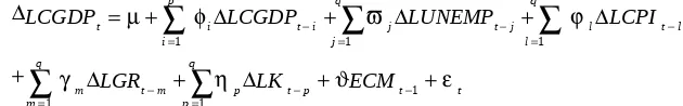
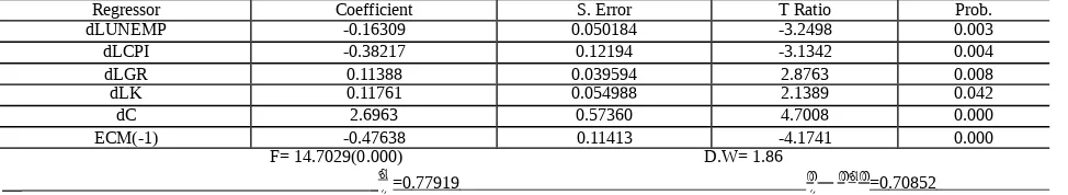
171Published by Canadian Center of Science and Education ISSN 1916-971X E-ISSN 1916-9728171 It is essential to look at unemployment rate and per capita real GDP trends in Iran for the period ranging from 1971 to 2006(Figure 1 & 2).
The paper is organized in V Sections. Section II summarizes some recent literature on the subject. Section III explains data and mathematical model employed to capture the influence of macroeconomic factors on per capita real GDP. Section IV incorporates the empirical results of bounds testing procedure proposed by Pesaran. Section V concludes the study and discusses some implications for the current debate about the impacts of macroeconomic factors on per capita real GDP in general.
2. Review of literature
Villaverde and Maza (2009) analyze Okun’s law for the Spanish regions over the period 1980-2004. They found that an inverse relationship between unemployment and output holds for most of the regions and for the whole country. However, the quantitative values of Okun’s coefficients are quite different, a result that is partially explained by regional disparities in productivity growth. These differences imply that, when it comes to policy issues, conventional aggregate demand/supply management policies should be combined with region-specific policies. Zaleha et al. (2007) examine relationship between output and unemployment in the Malaysian economy. They found that the negative relationship between output and unemployment is present. They also found two-way causality between unemployment and output growth in Malaysia.
Christopoulos (2004) investigates the relationship between output and unemployment in Greece at a regional level through the implementation of Okun’s law. Current practice is primarily restricted to the national level, and thus ignores the regional dimension of this relationship. He uses modern unit root test and co-integration techniques based on panel data settings. The empirical results reveal that Okun’s law can be confirmed for six out of the 13 regions we examine.
Perman and Tavera (2004) examine for the presence of convergence of the Okun’s Law coefficient (OLC) among several alternative groupings of European economies. The empirical strategy adopted is based on the evaluation of the time path of rolling regression estimates of the OLC for European countries. They then use a testing procedure suggested by Evans (1996) to investigate the convergence, or non-convergence, of the OLC in several groups of European countries by examining how the cross-country variance of the OLC evolves over time in these groups. A hypothesis of medium-term convergence of the OLC is rejected for most of the European country groups examined. Gil-Alana (2002) investigates the presence of structural breaks in the US output and unemployment rate by means of using fractionally integrated techniques. The results indicate that, for unemployment, the inclusion of breaks does not affect to the degree of integration of the series, while for the GNP, they observe a reduction in its order of integration of about 0.25 when a break due to the oil price crisis is taken into account.
Dornbusch et.al (2001) argue that forgone output is the major cost of unemployment, and if the loss is very high it
could lead to recession.
Freeman (2001) uses new developments in trend/cycle decomposition to test Okun’s Law for a panel of ten industrial countries, finding that Okun’s original estimate for the U.S. of three points of real GDP growth for each one percent reduction in the unemployment rate now averages just under two points of real GDP growth for the sample countries. Also, he finds that omission of capital and labor inputs may have biased previous estimates. As Romer (2001) reports, there is a well-established stylized fact about the fluctuations in the US economy – that the employment rate is pro-cyclical and the unemployment rate counter-cyclical. During all the recessions in the 1947-1999 period he finds that the employment fell 3.6% on the average, and also that the rate shrank during each of the periods.
Balmaseda et al. (2000) use data for a sample of 16 OECD countries from 1950 to 1989 in order to assess the effect of aggregate demand, productivity, and labor supply shocks on the real output, real wages and the unemployment rate. They found that unemployment rate fluctuations are dominated by aggregate demand shocks in the short-run. Lee (2000) evaluates the robustness of the Okun relationship based on postwar data for 16 OECD countries. He uses two different approaches, the first-difference and the “gap” model. He finds statistically significant Okun’s coefficients for almost all countries, but some differences among the countries. Some countries are characterized by low absolute values of the coefficient, which he attributes mainly to rigidities in the labor market.
ww
w .ccsenet.o www .ccsenet.o rg/ijef rg/ijef International Journal of Economics and FinanceInternational Journal of Economics and Finance Vol. 3, No. 5; October 2011Vol. 3, No. 5; October 2011
ww
w .ccsenet.o www .ccsenet.o rg/ijef rg/ijef International Journal of Economics and FinanceInternational Journal of Economics and Finance Vol. 3, No. 5; October 2011Vol. 3, No. 5; October 2011
173Published by Canadian Center of Science and Education ISSN 1916-971X E-ISSN 1916-9728173 Prachowny (1993) found that changes in output will result in changes in efficiency of production. Other important determinants of output include the amount of time worked and exploitation of facility space.
Watts and Mitchell (1991) supported Okun’s law. According to their study, the long-term relationship between unemployment and capacity utilization is not stable. Factors such as increasing labor resource utilization weaken the estimations of Okun’s law.
Evans (1989) uses data for the US economy from 1950 to 1989 in order to assess the relationship between the GDP growth and the unemployment rate. He finds a “substantial feedback” between the two variables, supported by the contemporaneous correlation between them. Using a non-restricted bivariate VAR he shows that there is a long-run relationship between the GDP growth and unemployment at about 0.30, in line with Okun’s findings.
Hamada and Kurosaka (1984) study the question whether the celebrated “Okun’s law”, a relation between excess capacity and unemployment, applies to the postwar Japanese economy. The coefficient that measures the responsiveness of the output gap to the unemployment rate is very large, reaching 28. This large coefficient can be attributed to the elastic response in the female participation ratio, to flexible working hours, to the slow adjustment in employment, and to changes in industrial structures.
Although the empirical study of Okun’s law has indeed blossomed since the publication of Prachowny’s paper (1993), most of it only deals with data at national level. Fortunately, in the last few years some studies have tried to overcome this shortcoming, thus introducing a regional dimension in the analysis of the relationship between output and unemployment.
3. Method
There are several methods available to test for the existence of the long-run equilibrium relationship among time-series variables. The most widely used methods include Engle and Granger (1987) test, fully modified OLS procedure of Phillips and Hansen’s (1990), maximum likelihood based Johansen (1988,1991) and Johansen-Juselius (1990) tests. These methods require that the variables in the system are integrated of order one I(1). In addition, these methods suffer from low power and do not have good small sample properties. Due to these problems, a newly developed autoregressive distributed lag (ARDL) approach to co-integration has become popular in recent years. This study employs autoregressive distributed lag approach (ARDL) to co-integration following the methodology proposed by Pesaran and Shin (1999). This methodology is chosen as it has certain advantages on other cointegration procedures. First, the series used do not have to be I(1) (Pesaran & Pesaran, 1997). Second, even with small samples more efficient cointegration relationships can be determined (Ghatak & Siddiki, 2001). Finally, the ARDL approach overcomes the problems resulting from non-stationary time series data leading to spurious regression coefficient that are biased towards zero (Stock & Watson, 1993).
First of all data has been tested for unit root. This testing is necessary to avoid the possibility of spurious regression as Ouattara (2004) reports that bounds test is based on the assumption that the variables are I(0) or I(1) so in the presence of I(2) variables the computed F-statistics provided by Pesaran et al. (2001) becomes invalid. Similarly other diagnostic tests are applied to detect serial correlation, heteroscedasticity , conflict to normality.
If data is found I(0) or I(1) the ARDL approach to co-integration is applied which consists of three stages. In the first step the existence of a long-run relationship between the variables is established by testing for the significance of lagged variables in an error correction mechanism regression. Then the first lags of the levels of each variable are added to the equation to create the error correction mechanism equation and a variable addition test is performed by computing an F-test on the significance of all the lagged variables.
The second stage is to estimate the ARDL form of equation where the optimal lag length is chosen according to one of the standard criteria such as the Akaike Information or Schwartz Bayesian. Then the restricted version of the equation is solved for the long-run solution. An ARDL representation of above equation is as below:
ww
w .ccsenet.o www .ccsenet.o rg/ijef rg/ijef International Journal of Economics and FinanceInternational Journal of Economics and Finance Vol. 3, No. 5; October 2011Vol. 3, No. 5; October 2011
174Published by Canadian Center of Science and Education ISSN 1916-971X E-ISSN 1916-9728174 CGDP = Per Capita Real GDP
GR = Ratio of Government Expenditure to GDP K= Physical Capital
The third stage entails the estimation of the error correction equation using the differences of the variables and the lagged long-run solution, and determines the speed of adjustment of returns to equilibrium. A general error
and are the short-run dynamic coefficients of the model’s convergence to equilibrium and is
the speed of adjustment. The F-test is used for testing the existence of long-run relationship. When long-run relationship exist, F-test indicates which variable should be normalized. The null hypothesis for no co-integration
among variables is H 0 : 1 2 3 4 5
0
against the alternative hypothesis
H1 :
1
2
3
4
5 0 . The F-test has a non-standard distribution which depends on (i) whethervariables included in the model are I(0) or I(1), (ii) the number of regressors, and (iii) whether the model contains an intercept and/or a trend. Given a relatively small samples size, the critical values used are as reported by Narayan(2004) which based on small sample size between 30 and 80. The test involves asymptotic critical value bounds, depending whether the variables are I(0) or I(1) or mixture of both. Two sets of critical values are generated which one set refers to the I(1) series and the other for the I(0) series. Critical values for the I(1) series are referred to as upper bound critical values, while the critical values for I(0) series are referred to as the lower bound critical values.
If the F-test statistic exceeds their respective upper critical values, we can conclude that there is evidence of a long-run relationship between the variables regardless of the order of integration of the variables. If the test statistic is below the upper critical value, we cannot reject the null hypothesis of no co-integration and if it lies between the bounds, a conclusive inference cannot be made without knowing the order of integration of the underlying regressors.
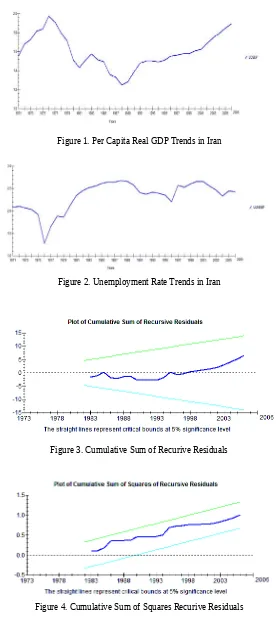
To complement this study it is important to investigate whether the above long run relationship we found are stable for the entire period of study. In other words, we have to test for parameter stability. The methodology used here is based on the cumulative sum (CUSUM) and the cumulative sum of squares (CUSUMSQ) tests proposed by Brown
et al. (1975). Unlike the Chow test, that requires break point(s) to be specified, the CUSUM tests can be used even if we do not know the structural break point. The CUSUM test uses the cumulative sum of recursive residuals based on the first n observations and is updated recursively and plotted against break point. The CUSUMSQ makes use of the squared recursive residuals and follows the same procedure. If the plot of the CUSUM and CUSUMSQ stays within the 5 percent critical bound the null hypothesis that all coefficients are stable cannot be rejected. If however, either of the parallel lines are crossed then the null hypothesis (of parameter stability) is rejected at the 5 percent significance level.
4. Results
Table 1 reports the results of unit root test applied to determine the order of integration among time series data. ADF Test has been used at level and first difference under assumption of constant and trend.
Results clearly indicate that the index series except for unemployment rate are not stationary at level but the first differences of the logarithmic transformations of the series are stationary. Therefore, it can be safely said that series are integrated of order one I(1). As suggested by Pesaran and Shin(1999) and Narayan(2004), since the observations are annual, we choose 2 as the maximum order of lags in the ARDL and estimate for the period of 1971-2006. In fact, we also used the Schwarz-Bayesian criteria (SBC) to determine the optimal number of lags to be included in the conditional ECM(error correction model), whilst ensuring there was no evidence of serial correlation, as emphasized by Pesaran et al.(2001).
Table 2 indicates that macroeconomic variables significantly explain per capita real GDP. The value of R-Bar-Squared is 0.95 which indicates a high degree of correlation among variables.
After analyzing the bound test for co-integration, next step is to estimate the coefficient of the long-run relationships.
Table 3 displays the results long-run coefficients under ARDL approach. Results reveal that unemployment rate, the physical capital, the consumer price index and the ratio of government expenditure to GDP have significant long-run effect on per capita real GDP.
The unemployment rate and the consumer price index are significantly negatively related with per capita real GDP which are logical as increase in these variables leads to increase in per capita real GDP. The physical capital and the ratio of government expenditure to GDP are significantly positively related with per capita real GDP.
Error Correction Representation of above long-run relationship is reported in Table 4 which captures the short-run dynamics of relationship among macroeconomic variables and per capita real GDP. The error correction model
based upon ARDL approach establishes that changes in unemployment rate, the physical capital, the consumer price
index and the ratio of government expenditure to GDP have significant short-run effect.
According to results short-run elasticities of unemployment rate, the consumer price index, the ratio of government expenditure to GDP and the physical capital are -0.16, -0.38, 0.11 and 0.12 respectively. It is worth mentioning that these elasticities are much lower than long run elasticities. ECM(-1) is one period lag value of error terms that are obtained from the long-run relationship. The coefficient of ECM(-1) indicates how much of the disequilibrium in the short-run will be fixed (eliminated) in the long-run.
As expected, the error correction variable ECM(-1) has been found negative and also statistically significant. The Coefficient of the ECM term suggests that adjustment process is quite fast and 47% of the previous year’s disequilibrium in per capita real GDP from its equilibrium path will be corrected in the current year.
Finally, CUSUM and CUSUMSQ plots are drawn to check the stability of short-run and long-run coefficients in the ARDL error correction model. Figure 3 & 4 show that both CUSUM and CUSUMSQ are within the critical bounds of 5% so it indicates that the model is structurally stable.
5. Discussion and conclusion
This study examines the relationship between the unemployment rate and per capita real GDP for the period 1971 to 2006 by using autoregressive distributed lag approach based on bounds testing procedure proposed by Pesaran and Shin (2001).
Unit root test clearly indicate that the index series except for unemployment rate are not stationary at level but the first differences of the logarithmic transformations of the series are stationary.
Results of ARDL long-run coefficients reveal that unemployment rate, the physical capital, the consumer price index and the ratio of government expenditure to GDP are statistically significant in determining per capita real GDP in the long-run. The error correction model based upon ARDL approach indicates that changes in the above-mentioned variables are statistically significant in the short-run.
Based on the results of short-run and long-run, the unemployment rate and the consumer price index are negatively related with per capita real GDP, while the physical capital and the ratio of government expenditure to GDP are positively related with per capita real GDP.
The error correction variable ECM(-1) has been found negative and statistically significant. The Coefficient of the ECM term suggests that adjustment process is quite fast and 47% of the previous year’s disequilibrium in per capita real GDP from its equilibrium path will be corrected in the current year. CUSUM and CUSUMSQ plots are drawn to check the stability of short run and long run coefficients in the ARDL error correction model and . CUSUM and CUSUMSQ are within the critical bounds of 5% that indicates that the model is structurally stable.
References
Balmaseda, M., Dolado, J. and López-Salido, J.D. (2000). The dynamic effects of shocks to labour markets:
evidence from OECD countries, Oxford Economic Papers, 52, 3-23. doi:10.1093/oep/52.1.3,
h tt p :// dx .d o i. o r g / 1 0 . 1 09 3 /oep/52.1.3
Brown, R.L., Durbin, J. and Evans, J.M. (1975). Techniques for Testing the Consistency of Regression Relations
Over Time, Journal of the Royal Statistical Society, 37, 149-92.
Chen, D.(2008). Country report, Economic Research Department.
Christopoulos, D. (2004) The relationship between output and unemployment: Evidence from Greek regions, Papers in Regional Science, 83, 611-620. doi:10.1111/j.1435-5597.2004.tb01928.x,
Dornbusch, R., Fosher, S. and Startz, R. (2001). Macroeconomics, McGraw-Hill.
Engle, R. F. and Granger, C. W. J.(1987). Co-integration and Error Correction: Representation, Estimation and
Testing, Econometrica, 55, 251-276. doi:10.2307/1913236 h tt, p ://d x .d o i. o r g / 1 0 .2 3 0 7 /1913236
Evans, M.D.R. (1989). Immigrant Entrepreneurship: Effects of Ethnic Market Size and Isolated Labor Pool,
American Sociological Review, 54, 950-962. doi:10.2307/2095717, h tt p : // dx . do i .o r g / 1 0.2 3 0 7 /2095717
Freeman, D.G. (2001). Panel Tests of Okun’s Law for Ten Industrial Countries, Economic Inquiry, 39, 511-513.
doi:10.1093/ei/39.4.511, h tt p :// dx .d o i.or g / 1 0 . 1 09 3 /ei/39.4.511
Ghatak, S. and Siddiki, J. (2001). The use of ARDL approach in estimating virtual exchange rates in India, Journal
of Applied Statistics, 28, 573-583. doi:10.1080/02664760120047906,
h tt p :// dx .d o i. o r g / 1 0 . 1 08 0 /02664760120047906
Gil-Alana, L. (2002). Structural breaks and fractional integration in the US output and unemployment rate, Economics Letters, 77, 79-84. doi:10.1016/S0165-1765(02)00106-4,
h tt p :// dx .d o i. o r g / 1 0 . 1 01 6 /S0165-1765(02)00106-4
Hamada, K. and Kurosaka, Y. (1984). The relationship between production and unemployment in Japan: Okun’s law in comparative perspective, European Economic Review, 25(1), 71-94. doi:10.1016/0014-2921(84)90073-4,
h tt p :// dx .d o i. o r g / 1 0 . 1 01 6 /0014-2921(84)90073-4
Johansen, S. (1988). Statistical analysis of co-integration vectors, Journal of Economic Dynamics and Control, 12, 231-254. doi:10.1016/0165-1889(88)90041-3, htt p ://d x . do i .or g / 1 0.10 16 /0165-1889(88)90041-3
Johansen, S. and Juselius, K.(1990). Maximum likelihood estimation and inference on co-integration with applications to the demand for money, Oxford Bulletin of Economics and Statistics, 51, 169–210
Johansen, S.(1991). Estimation and Hypothesis Testing of Co-integration Vectors in Gaussian Vector
Autoregressive Models, Econometrica, 59(6),1551-1580. doi:10.2307/2938278, h tt p ://d x . do i .or g / 1 0.230 7 /2938278
Lee, J. (2000). The Robustness of Okun’s Law: Evidence from OECD Countries, Journal of Macroeconomics, 22,
331-56. doi:10.1016/S0164-0704(00)00135-X, h tt p :// d x.d o i . or g / 1 0.10 16 /S0164-0704(00)00135-X
Narayan, P.K. (2004). Reformulating critical values for the bounds F-statistics approach to co-integration: an application to the tourism demand model for Fiji, Department of Economics Discussion Papers, No.2,pp.4.
Ouattara, B. (2004a). The Impact of Project Aid and Program Aid on Domestic Savings: A Case Study of Côte d'Ivoire, Centre for the Study of African Economies Conference on Growth, Poverty Reduction and Human Development in Africa.
Ouattara, B. (2004b). Foreign Aid and Fiscal Policy in Senegal, Mimeo University of Manchester.
Perman, R. and Tavera, C. (2004) .Testing for convergence of the Okun’s law coefficient in Europe, Discussion Papers in Economics, 04-12, University of Stractchclyde.
Pesaran, M. H. and Pesaran, B. (1997). Working with Microsoft 4.0, Camfit data Ltd, Cambridge.
Pesaran and Shin (1999). An autoregressive distributed lag modeling approach to co-integration analysis. DAE Working papers, No.9514.
Pesaran, M., Shin, Y. and Richard, J.S. (2001). Bounds testing approaches to the analysis of level relationships,
Journal of Applied Econometrics, 16(3), 289-326. doi:10.1002/jae.616, ht t p ://dx .d o i. or g/1 0 . 1002/jae.616
Phillips, P.C.B. and Hansen, B.E. (1990). Statistical Inference in Instrumental Variables Regression with I(1) Processes, Review of Economic Studies, 57, 99-125. doi:10.2307/2297545, h tt p :// d x. do i .or g / 1 0.23 07 /2297545
Prachowny, M.F.J. (1993). Okun’s Law: Theoretical Foundations and Revisited Estimates, Review of Economics
and Statistics, 75, 331-335. doi:10.2307/2109440, h tt p ://d x . do i.or g / 1 0.230 7 /2109440 Romer, D. (2001). Advanced Macroeconomics, 2nd edition, New York: McGraw-Hill/Irwin.
Shayerah, I. (2010). Iran’s Economic Conditions: U.S. Policy Issues, Congressional Research Service.
Stock, J. H. and Watson, M. (1993). A simple estimator of co-integrating vectors in higher order integrated systems.
Villaverde, J. and Maza, A. (2009). The robustness of Okun’s Law in Spain, 1980–2004: Regional evidence,
Journal of Policy Modeling, 31(2), 289-297. doi:10.1016/j.jpolmod.2008.09.003,
h tt p :// dx .d o i. o r g / 1 0 . 1 01 6 /j.jpolmod.2008.09.003
Watts, M. and Mitchell, W. (1991). Alleged Instability of the Okun’s Law Relationship in Australia, Applied
Economics, 23, 1829-1838. doi:10.1080/00036849100000172, h tt p ://d x . do i .or g / 1 0.10 80 /00036849100000172
Weber, C.E. (1995). Cyclical Output, Cyclical Unemployment, and Okun’s Coefficient: A New Approach. Journal
of Applied Econometrics, 10, 433-445. doi:10.1002/jae.3950100407, h tt p :// dx .d o i.or g / 1 0 . 1 00 2 /jae.3950100407 Zaleha, M., Norashidah, M. and Judhiana, A. (2007) The Relationship between Output and Unemployment in
Malaysia: Does Okun’s Law exist?, Unemployment in Malaysia: Does Okun’s Law exist?, International Journal of
Economics and Management, 1(3),337–344.
Table1. Unit Root Analysis
intercept but not a trend intercept and a linear trend Variable ADF-Level ADF-Ist Diff ADF-Level ADF-Ist Diff 5% Critic Value -2.9665 -2.9706 -3.5731 -3.5796
Table 2. ARDL(1,1,0,0,1) selected based on SBC
Table 3. Estimated Long Run Coefficients for selected ARDL Model
Regressor Coefficient S. Error T Ratio Prob.
Table 4. Error Correction Representation for the Selected ARDL Model
Figure 1. Per Capita Real GDP Trends in Iran
Figure 2. Unemployment Rate Trends in Iran
Figure 3. Cumulative Sum of Recurive Residuals
Figure 4. Cumulative Sum of Squares Recurive Residuals
abstrak
ini, modal fisik , indeks harga konsumen dan rasio pengeluaran pemerintah terhadap PDB sebagai variabel kontrol telah dipertimbangkan . Temuan menunjukkan bahwa tingkat pengangguran memiliki pengaruh yang signifikan dan negatif pada PDB per kapita riil dalam jangka panjang dan jangka pendek . Nilai koefisien koreksi kesalahan sebesar -0.48
menyiratkan bahwa sekitar 95 % dari GDP per kapita penyesuaian nyata terjadi setelah dua tahun .
Kata kunci : Tingkat pengangguran , PDB per kapita riil , Auto - regresif Distributed Lag ( ARDL ) , mekanisme koreksi kesalahan
1 . Pendahuluan
Pengangguran merupakan masalah penting di negara berkembang. Pengangguran yang tinggi berarti bahwa sumber daya tenaga kerja tidak digunakan secara efisien . Oleh karena itu , kesempatan kerja penuh harus menjadi tujuan makroekonomi utama dari setiap pemerintah karena memaksimalkan output.
Sistem bivariat output dan tingkat pengangguran adalah salah satu yang paling sering dipelajari dalam tradisi VAR untuk menganalisis propagasi dan kegigihan guncangan dalam ekonomi riil dan mekanisme transmisi antara produk dan pasar tenaga kerja .
Republik Islam Iran adalah negara terbesar kedua di Timur Tengah. Dengan PDB per kapita berdiri di USD
3610 pada tahun 2007 , negara ini diklasifikasikan oleh Bank Dunia sebagai negara berpendapatan menengah ke bawah .
Perekonomian Iran telah mengalami pertumbuhan yang kuat , dengan PDB riil rata-rata 5,6 % selama lima tahun terakhir . Kinerja yang kuat terutama didukung oleh harga minyak yang tinggi dan stimulan fiskal . Faktor-faktor ini akan terus mendukung perekonomian Iran pada periode perkiraan kami . Di sisi permintaan , konsumsi swasta dan investasi akan sangat mendukung pertumbuhan . Namun, konsumsi swasta akan terhambat oleh melonjaknya inflasi . Investasi akan tetap kuat , tetapi menghadapi risiko penurunan yang signifikan . Rasa takut serangan militer telah mereda setelah rilis laporan intelijen AS menyimpulkan bahwa Iran mengembangkan senjata nuklir mereda pada tahun 2003 ( Chen , 2008) .
Beberapa pengamat berpendapat bahwa tingkat pengangguran lebih tinggi dari angka yang dilaporkan oleh pemerintah Iran . Tingkat pengangguran tetap tinggi , mencapai 11,8 % diperkirakan pada tahun 2008 . Setidaknya seperlima dari Iran hidup di bawah garis kemiskinan pada tahun 2002 . Iran memiliki penduduk muda dan setiap tahun , sekitar 750.000 warga Iran memasuki pasar kerja untuk pertama kalinya , menempatkan tekanan pada pemerintah untuk menciptakan lapangan kerja baru . Emigrasi orang-orang muda yang terampil dan
berpendidikan terus menimbulkan masalah bagi Iran . IMF melaporkan bahwa Iran memiliki tertinggi " brain drain " tingkat di dunia ( Shayerah 2010 )
Tujuan dari makalah ini adalah untuk menawarkan penyelidikan statistik menyeluruh dinamika gabungan output dan tingkat pengangguran .
Hal ini penting untuk melihat tingkat pengangguran dan per kapita tren GDP riil di Iran untuk periode mulai 1971-2006 ( Gambar 1 & 2 ) .
Makalah ini disusun dalam Bagian V . Bagian II meringkas beberapa literatur terbaru pada subjek. Bagian III menjelaskan data dan model matematika yang digunakan untuk menangkap pengaruh faktor ekonomi makro pada PDB per kapita riil . Bagian IV menggabungkan hasil empiris prosedur batas pengujian yang diusulkan oleh Pesaran . Bagian V menyimpulkan penelitian dan membahas beberapa implikasi bagi perdebatan saat ini tentang dampak dari faktor ekonomi makro pada per kapita PDB riil pada umumnya .
2 . Ulasan sastra
Villaverde dan Maza (2009) menganalisis hukum Okun untuk wilayah Spanyol selama periode 1980-2004 . Mereka menemukan bahwa hubungan terbalik antara pengangguran dan output berlaku untuk sebagian besar wilayah dan untuk seluruh negeri . Namun, nilai-nilai kuantitatif koefisien Okun sangat berbeda , hasil yang sebagian dijelaskan oleh perbedaan regional dalam pertumbuhan produktivitas . Perbedaan ini menyiratkan bahwa , ketika datang ke isu-isu kebijakan , kebijakan manajemen permintaan agregat / pasokan konvensional harus dikombinasikan dengan kebijakan daerah yang spesifik .
Zaleha et al . ( 2007) meneliti hubungan antara output dan pengangguran dalam ekonomi Malaysia . Mereka menemukan bahwa hubungan negatif antara output dan pengangguran hadir . Mereka juga menemukan dua arah kausalitas antara pengangguran dan pertumbuhan output di Malaysia .
Christopoulos ( 2004) menyelidiki hubungan antara output dan pengangguran di Yunani pada tingkat regional melalui penerapan hukum Okun . Praktek saat ini terutama terbatas pada tingkat nasional , dan dengan demikian mengabaikan dimensi regional hubungan ini . Dia menggunakan akar unit test dan co - integrasi teknik-teknik modern berdasarkan pengaturan data panel . Hasil empiris menunjukkan bahwa hukum Okun dapat dikonfirmasi untuk enam dari 13 daerah kita kaji .
kelompok negara-negara Eropa dengan memeriksa bagaimana varians lintas negara dari OLC berkembang dari waktu ke waktu dalam kelompok ini . Sebuah hipotesis konvergensi jangka menengah dari OLC ditolak untuk sebagian besar kelompok negara Eropa diperiksa . Gil - Alana ( 2002 ) menyelidiki adanya istirahat struktural dalam output AS dan tingkat pengangguran dengan cara menggunakan teknik fraksional terintegrasi . Hasil penelitian menunjukkan bahwa , pengangguran , dimasukkannya istirahat tidak berpengaruh terhadap tingkat integrasi dari seri , sedangkan untuk GNP , mereka mengamati penurunan order integrasi dari sekitar 0,25 ketika istirahat akibat krisis harga minyak diperhitungkan . Dornbusch et.al ( 2001) menyatakan bahwa output yang hilang adalah biaya utama dari pengangguran , dan jika kerugian yang sangat tinggi bisa menyebabkan resesi .
Freeman ( 2001) menggunakan perkembangan baru dalam dekomposisi trend / siklus untuk menguji Hukum Okun untuk panel sepuluh negara industri , menemukan bahwa perkiraan semula Okun bagi AS dari tiga poin dari pertumbuhan PDB riil untuk setiap penurunan satu persen dalam tingkat pengangguran sekarang rata-rata hanya di bawah dua poin dari
pertumbuhan PDB riil bagi negara-negara sampel . Selain itu, ia menemukan bahwa kelalaian modal dan tenaga kerja input mungkin bias perkiraan sebelumnya .
Seperti yang dilaporkan Romer ( 2001) , ada fakta bergaya mapan tentang fluktuasi ekonomi AS - bahwa tingkat kerja pro -cyclical dan tingkat pengangguran counter-cyclical . Selama resesi di
Periode 1947-1999 ia menemukan bahwa pekerjaan tersebut turun 3,6 % rata-rata , dan juga bahwa tingkat menyusut selama setiap periode .
Balmaseda et al . (2000) menggunakan data untuk sampel dari 16 negara OECD 1950-1989 untuk menilai efek dari permintaan agregat , produktivitas , dan guncangan penawaran tenaga kerja pada output riil , upah riil dan tingkat pengangguran . Mereka menemukan bahwa fluktuasi tingkat pengangguran didominasi oleh guncangan permintaan agregat dalam jangka pendek .
Lee (2000) mengevaluasi ketahanan hubungan Okun berdasarkan data pascaperang untuk 16 negara OECD . Dia menggunakan dua pendekatan yang berbeda , pertama - perbedaan dan " gap " model . Dia menemukan koefisien signifikan secara statistik Okun untuk hampir semua negara , tetapi beberapa perbedaan antara negara-negara . Beberapa negara yang ditandai oleh nilai-nilai absolut yang rendah koefisien , yang ia atribut terutama untuk kekakuan dalam pasar tenaga kerja .
Weber ( 1995) menggunakan empat metode yang berbeda untuk mengekstrak komponen siklus output dan pengangguran . Dia menggunakan komponen siklis untuk mendapatkan estimasi koefisien Okun untuk ekonomi AS selama periode 1948-1988. Ia menemukan bahwa nilai-nilai rentang koefisien dari -0.22 sampai -0.31, sehingga bertentangan klaim bahwa
Koefisien Okun agak stabil sekitar nilai -0.3.
Prachowny ( 1993) menemukan bahwa perubahan dalam output akan menghasilkan perubahan dalam efisiensi produksi . Determinan penting lainnya output meliputi jumlah waktu bekerja dan eksploitasi ruang fasilitas .
Watts dan Mitchell ( 1991) didukung hukum Okun . Menurut penelitian mereka , hubungan jangka panjang antara pengangguran dan pemanfaatan kapasitas tidak stabil . Faktor-faktor seperti peningkatan pemanfaatan sumber daya tenaga kerja melemahkan estimasi hukum Okun . Evans ( 1989) menggunakan data ekonomi AS 1950-1989 untuk menilai hubungan antara pertumbuhan PDB dan tingkat pengangguran . Dia menemukan " umpan balik yang cukup besar " antara kedua variabel , yang didukung oleh korelasi kontemporer di antara mereka . Menggunakan bivariat VAR non - Pembatasan ia menunjukkan bahwa ada hubungan jangka panjang antara pertumbuhan PDB dan pengangguran sekitar 0,30 , sejalan dengan temuan Okun .
Hamada dan Kurosaka ( 1984) mempelajari pertanyaan apakah merayakan " hukum Okun " itu , hubungan antara kelebihan kapasitas dan pengangguran , berlaku untuk ekonomi Jepang pascaperang . Koefisien yang mengukur respon dari output gap dengan tingkat pengangguran yang sangat besar, mencapai 28 . Koefisien besar ini dapat dikaitkan dengan respon elastis dalam rasio partisipasi perempuan , dengan jam kerja yang fleksibel , penyesuaian lambat dalam pekerjaan , dan perubahan dalam struktur industri .
Meskipun studi empiris hukum Okun memang berkembang sejak penerbitan kertas Prachowny (1993 ) , sebagian besar hanya berhubungan dengan data pada tingkat nasional . Untungnya , dalam beberapa tahun terakhir beberapa studi telah mencoba untuk mengatasi kekurangan ini , sehingga memperkenalkan dimensi regional dalam analisis hubungan antara output dan pengangguran .
3 . Metode
pendekatan autoregressive distributed lag ( ARDL ) untuk bersama - integrasi mengikuti metodologi yang diusulkan oleh Pesaran dan Shin ( 1999) . Metodologi ini dipilih karena memiliki kelebihan tertentu pada prosedur kointegrasi lainnya . Pertama , seri yang digunakan tidak harus I ( 1 ) ( Pesaran & Pesaran , 1997) . Kedua , bahkan dengan sampel kecil hubungan kointegrasi yang lebih efisien dapat ditentukan ( Ghatak & Siddiki , 2001 ) . Akhirnya , pendekatan ARDL mengatasi masalah yang dihasilkan dari data time series non - stasioner menyebabkan koefisien regresi palsu yang bias menuju nol ( Stock & Watson , 1993) . Pertama-tama data yang telah diuji untuk unit root . Pengujian ini diperlukan untuk
menghindari kemungkinan regresi palsu sebagai Ouattara ( 2004 ) melaporkan bahwa uji batas didasarkan pada asumsi bahwa variabel I ( 0 ) atau I ( 1 ) sehingga di hadapan saya ( 2 ) variabel yang dihitung F -statistik yang disediakan oleh Pesaran et al . ( 2001) menjadi tidak valid . Demikian pula tes diagnostik lainnya diterapkan untuk mendeteksi korelasi serial , heteroskedastisitas , konflik ke keadaan normal .
Jika data ditemukan I ( 0 ) atau I ( 1 ) pendekatan ARDL untuk co - integrasi diterapkan yang terdiri dari tiga tahap . Pada langkah pertama adanya hubungan jangka panjang antara variabel didirikan dengan menguji signifikansi variabel tertinggal dalam regresi kesalahan mekanisme koreksi . Kemudian kelambatan pertama dari tingkat masing-masing variabel ditambahkan ke persamaan untuk membuat kesalahan koreksi persamaan mekanisme dan tes tambahan variabel dilakukan dengan menghitung F -test pada signifikansi semua variabel tertinggal .
Tahap kedua adalah untuk memperkirakan bentuk ARDL persamaan di mana panjang lag optimal dipilih sesuai dengan salah satu kriteria standar seperti Informasi Akaike atau Schwartz Bayesian . Kemudian versi terbatas dari persamaan diselesaikan untuk solusi jangka panjang . Sebuah representasi ARDL dari persamaan di atas adalah sebagai berikut :
Keterangan :
CGDP = Per Kapita PDB UNEMP = Tingkat Pengangguran CPI = Indeks Harga Konsumen
GR = Rasio Pengeluaran Pemerintah terhadap PDB K = Modal Fisik
Tahap ketiga memerlukan estimasi persamaan koreksi kesalahan menggunakan perbedaan variabel dan
tertinggal solusi jangka panjang, dan menentukan kecepatan penyesuaian kembali ke
keseimbangan. Sebuah representasi koreksi kesalahan umum persamaan diberikan di bawah ini:
Keterangan :
, , , ,
dan adalah jangka pendek koefisien dinamis konvergensi model untuk kesetimbangan dan adalah
kecepatan penyesuaian . The F -test digunakan untuk menguji adanya hubungan jangka panjang . Ketika hubungan jangka panjang ada, F -test menunjukkan variabel yang harus dinormalisasi . Hipotesis nol tanpa co - integrasi
antar variabel adalah
H 0 : 1 2 3 4 5 0
melawan hipotesis alternatif
atas , sedangkan nilai-nilai penting bagi saya ( 0 ) seri disebut sebagai nilai kritis terikat lebih rendah .
Jika statistik F -test melebihi nilai kritis atas masing-masing , kita dapat menyimpulkan bahwa ada bukti hubungan jangka panjang antara variabel terlepas dari urutan integrasi variabel . Jika statistik uji berada di bawah nilai kritis atas , kita tidak dapat menolak hipotesis nol tidak ada co - integrasi dan jika terletak di antara batas-batas , kesimpulan konklusif tidak dapat dibuat tanpa mengetahui urutan integrasi regressors mendasari .
Untuk melengkapi penelitian ini adalah penting untuk menyelidiki apakah atas hubungan jangka panjang kami menemukan stabil untuk seluruh periode penelitian . Dengan kata lain, kita harus menguji stabilitas parameter . Metodologi yang digunakan di sini didasarkan pada kumulatif sum ( CUSUM ) dan jumlah kumulatif kuadrat ( CUSUMSQ ) tes yang diusulkan oleh Brown et al . ( 1975) . Berbeda dengan uji Chow , yang membutuhkan break point ( s ) yang akan ditentukan , tes CUSUM dapat digunakan bahkan jika kita tidak tahu titik istirahat struktural . Tes CUSUM menggunakan jumlah kumulatif residual rekursif berdasarkan pengamatan n pertama dan diperbarui secara rekursif dan diplot terhadap break point . The CUSUMSQ memanfaatkan residual rekursif kuadrat dan mengikuti prosedur yang sama . Jika plot CUSUM dan CUSUMSQ tetap dalam 5 persen kritis terikat hipotesis nol bahwa semua koefisien yang stabil tidak dapat ditolak . Jika demikian, salah satu dari garis paralel disilangkan maka hipotesis nol ( stabilitas parameter ) ditolak pada tingkat signifikansi 5 persen .
4 . Hasil
Tabel 1 laporan hasil uji akar unit yang digunakan untuk menentukan urutan integrasi antara data time series . ADF Uji telah digunakan pada tingkat dan perbedaan pertama di bawah asumsi konstan dan trend .
Hasil jelas menunjukkan bahwa seri indeks kecuali untuk tingkat pengangguran yang tidak stasioner pada tingkat namun perbedaan pertama dari transformasi logaritmik dari seri yang stasioner . Oleh karena itu, dapat dengan aman mengatakan bahwa seri terintegrasi order satu I ( 1 ) . Seperti yang disarankan oleh Pesaran dan Shin ( 1999) dan Narayan ( 2004), karena pengamatan dilakukan setiap tahun , kita memilih 2 sebagai urutan maksimum kelambanan dalam ARDL dan perkiraan untuk periode 1971-2006. Bahkan , kami juga menggunakan kriteria Schwarz - Bayesian ( SBC ) untuk menentukan jumlah optimal dari tertinggal untuk dimasukkan dalam ECM bersyarat ( error correction model ) , sementara memastikan tidak ada bukti korelasi serial, seperti yang ditekankan oleh Pesaran et al . ( 2001) .
Tabel 2 menunjukkan bahwa variabel ekonomi makro secara signifikan menjelaskan kapita PDB riil per . Nilai
R - Bar - Squared adalah 0,95 yang menunjukkan tingkat tinggi korelasi antara variabel . The F -test digunakan untuk menguji adanya hubungan jangka panjang . Nilai F - statistik ( F - statistik = 4,856 ) lebih tinggi dari nilai batas atas kritis pada 5 per tingkat persen signifikansi ( 4,049 ) , menggunakan intercept dibatasi dan tidak ada trend . Namun F - statistik hanya lebih tinggi dari nilai kritis batas atas di level 10 persen signifikansi ( 4,084 ) , menggunakan intercept terbatas dan trend . Hal ini menunjukkan bahwa hipotesis nol tidak ada co - integrasi tidak dapat diterima pada 5 persen dan 10 persen per tingkat dan oleh karena itu , ada hubungan co - integrasi antar variabel.
Setelah menganalisis tes terikat untuk co - integrasi , langkah berikutnya adalah untuk memperkirakan koefisien hubungan jangka panjang .
Tabel 3 menunjukkan hasil jangka panjang koefisien bawah pendekatan ARDL . Hasil menunjukkan bahwa tingkat pengangguran , modal fisik , indeks harga konsumen dan rasio pengeluaran pemerintah terhadap PDB memiliki efek jangka panjang yang signifikan terhadap PDB per kapita riil .
Tingkat pengangguran dan indeks harga konsumen secara signifikan berhubungan negatif dengan PDB riil per kapita yang logis sebagai peningkatan variabel-variabel ini menyebabkan peningkatan PDB riil per kapita . Modal fisik dan rasio pengeluaran pemerintah terhadap PDB secara signifikan berhubungan positif dengan PDB per kapita riil .
Representasi Koreksi Kesalahan di atas jangka panjang hubungan dilaporkan dalam Tabel 4 yang menangkap dinamika jangka pendek hubungan antara variabel makroekonomi dan PDB riil per kapita . Kesalahan correction model berdasarkan pendekatan ARDL menetapkan bahwa perubahan dalam tingkat pengangguran , modal fisik , indeks harga konsumen dan rasio pengeluaran pemerintah terhadap PDB memiliki efek jangka pendek yang signifikan . Menurut hasil jangka pendek elastisitas tingkat pengangguran , indeks harga konsumen , rasio pengeluaran pemerintah terhadap PDB dan modal fisik adalah -0.16 , -0.38 , 0.11 dan 0.12 masing-masing. Perlu disebutkan bahwa elastisitas ini jauh lebih rendah daripada jangka panjang elastisitas . ECM ( -1 ) adalah salah satu nilai lag periode istilah error yang diperoleh dari hubungan jangka panjang . Koefisien ECM ( -1 ) menunjukkan berapa banyak
cukup cepat dan 47 % dari ketidakseimbangan tahun sebelumnya dalam PDB per kapita riil dari jalan keseimbangannya akan diperbaiki pada tahun berjalan .
Akhirnya , CUSUM dan plot CUSUMSQ tertarik untuk memeriksa stabilitas jangka pendek dan jangka panjang koefisien dalam model kesalahan koreksi ARDL . Gambar 3 & 4 menunjukkan bahwa kedua CUSUM dan CUSUMSQ berada dalam batas-batas kritis 5 % sehingga
menunjukkan bahwa model tersebut secara struktural stabil . 5 . Diskusi dan kesimpulan
Penelitian ini menguji hubungan antara tingkat pengangguran dan PDB per kapita riil untuk periode 1971 hingga
2006 dengan menggunakan pendekatan autoregressive lag didistribusikan berdasarkan prosedur batas pengujian yang diusulkan oleh Pesaran dan
Shin ( 2001) .
Uji unit root jelas menunjukkan bahwa seri indeks kecuali untuk tingkat pengangguran yang tidak stasioner pada tingkat namun perbedaan pertama dari transformasi logaritmik dari seri yang stasioner .
Hasil ARDL jangka panjang koefisien mengungkapkan bahwa tingkat pengangguran , modal fisik , indeks harga konsumen dan rasio pengeluaran pemerintah terhadap PDB secara statistik signifikan dalam menentukan PDB riil per kapita dalam jangka panjang . Kesalahan correction model berdasarkan pendekatan ARDL menunjukkan bahwa perubahan dalam variabel yang disebutkan di atas secara statistik signifikan dalam jangka pendek .