CHAPMAN & HALL/CRC
Computational
Statistics
Handbook with
M
ATLAB
®
Wendy L. Martinez
Angel R. Martinez
This book contains information obtained from authentic and highly regarded sources. Reprinted material is quoted with permission, and sources are indicated. A wide variety of references are listed. Reasonable efforts have been made to publish reliable data and information, but the author and the publisher cannot assume responsibility for the validity of all materials or for the consequences of their use.
Neither this book nor any part may be reproduced or transmitted in any form or by any means, electronic or mechanical, including photocopying, microfilming, and recording, or by any information storage or retrieval system, without prior permission in writing from the publisher.
The consent of CRC Press LLC does not extend to copying for general distribution, for promotion, for creating new works, or for resale. Specific permission must be obtained in writing from CRC Press LLC for such copying.
Direct all inquiries to CRC Press LLC, 2000 N.W. Corporate Blvd., Boca Raton, Florida 33431. Trademark Notice: Product or corporate names may be trademarks or registered trademarks, and are used only for identification and explanation, without intent to infringe.
Visit the CRC Press Web site at www.crcpress.com © 2002 by Chapman & Hall/CRC
No claim to original U.S. Government works International Standard Book Number 1-58488-229-8 Printed in the United States of America 1 2 3 4 5 6 7 8 9 0
Printed on acid-free paper
To
Table of Contents
Preface
Chapter 1
Introduction
1.1 What Is Computational Statistics? 1.2 An Overview of the Book
Philosophy What Is Covered A Word About Notation 1.3 MATLAB Code
Computational Statistics Toolbox Internet Resources
1.4 Further Reading
Chapter 2
Probability Concepts
2.1 Introduction 2.2 Probability
Background Probability
Axioms of Probability
2.3 Conditional Probability and Independence Conditional Probability
Independence Bayes Theorem 2.4 Expectation
Mean and Variance Skewness
Kurtosis
2.5 Common Distributions Binomial
Multivariate Normal 2.6 MATLAB Code
2.7 Further Reading Exercises
Chapter 3
Sampling Concepts
3.1 Introduction
3.2 Sampling Terminology and Concepts Sample Mean and Sample Variance Sample Moments
Covariance
3.3 Sampling Distributions 3.4 Parameter Estimation
Bias
Mean Squared Error Relative Efficiency Standard Error
Maximum Likelihood Estimation Method of Moments
3.5 Empirical Distribution Function Quantiles
3.6 MATLAB Code
3.7 Further Reading Exercises
Chapter 4
Generating Random Variables
4.1 Introduction
4.2 General Techniques for Generating Random Variables Uniform Random Numbers
Inverse Transform Method Acceptance-Rejection Method
4.3 Generating Continuous Random Variables Normal Distribution
Exponential Distribution Gamma
Chi-Square Beta
Multivariate Normal
Generating Variates on a Sphere 4.4 Generating Discrete Random Variables
Binomial Poisson
4.5 MATLAB Code
4.6 Further Reading Exercises
Chapter 5
Exploratory Data Analysis
5.1 Introduction
5.2 Exploring Univariate Data Histograms
Stem-and-Leaf
Quantile-Based Plots - Continuous Distributions Q-Q Plot
Quantile Plots
Quantile Plots - Discrete Distributions Poissonness Plot
Binomialness Plot Box Plots
5.3 Exploring Bivariate and Trivariate Data Scatterplots
Surface Plots Contour Plots Bivariate Histogram 3-D Scatterplot
5.4 Exploring Multi-Dimensional Data Scatterplot Matrix
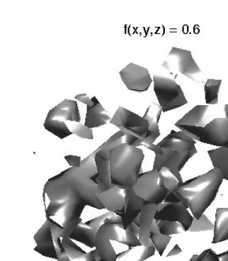
Slices and Isosurfaces Star Plots
Andrews Curves Parallel Coordinates Projection Pursuit
Projection Pursuit Index Finding the Structure Structure Removal Grand Tour
5.5 MATLAB Code
5.6 Further Reading Exercises
Chapter 6
Monte Carlo Methods for Inferential Statistics
6.1 Introduction
6.2 Classical Inferential Statistics Hypothesis Testing
Confidence Intervals
Basic Monte Carlo Procedure Monte Carlo Hypothesis Testing
Monte Carlo Assessment of Hypothesis Testing 6.4 Bootstrap Methods
General Bootstrap Methodology Bootstrap Estimate of Standard Error Bootstrap Estimate of Bias
Bootstrap Confidence Intervals
Bootstrap Standard Confidence Interval Bootstrap-t Confidence Interval
Bootstrap Percentile Interval 6.5 MATLAB Code
6.6 Further Reading Exercises
Chapter 7
Data Partitioning
7.1 Introduction 7.2 Cross-Validation 7.3 Jackknife
7.4 Better Bootstrap Confidence Intervals 7.5 Jackknife-After-Bootstrap
7.6 MATLAB Code
7.7 Further Reading Exercises
Chapter 8
Probability Density Estimation
8.1 Introduction 8.2 Histograms
1-D Histograms
Multivariate Histograms Frequency Polygons
Averaged Shifted Histograms 8.3 Kernel Density Estimation
Univariate Kernel Estimators Multivariate Kernel Estimators 8.4 Finite Mixtures
Univariate Finite Mixtures Visualizing Finite Mixtures Multivariate Finite Mixtures
EM Algorithm for Estimating the Parameters Adaptive Mixtures
8.7 Further Reading Exercises
Chapter 9
Statistical Pattern Recognition
9.1 Introduction
9.2 Bayes Decision Theory
Estimating Class-Conditional Probabilities: Parametric Method Estimating Class-Conditional Probabilities: Nonparametric Bayes Decision Rule
Likelihood Ratio Approach 9.3 Evaluating the Classifier
Independent Test Sample Cross-Validation
Receiver Operating Characteristic (ROC) Curve 9.4 Classification Trees
Growing the Tree Pruning the Tree Choosing the Best Tree
Selecting the Best Tree Using an Independent Test Sample Selecting the Best Tree Using Cross-Validation
9.5 Clustering
Measures of Distance Hierarchical Clustering K-Means Clustering 9.6 MATLAB Code
9.7 Further Reading Exercises
Chapter 10
Nonparametric Regression
10.1 Introduction 10.2 Smoothing
Loess
Robust Loess Smoothing Upper and Lower Smooths 10.3 Kernel Methods
Nadaraya-Watson Estimator Local Linear Kernel Estimator 10.4 Regression Trees
Growing a Regression Tree Pruning a Regression Tree Selecting a Tree
10.5 MATLAB Code
Exercises
Chapter 11
Markov Chain Monte Carlo Methods
11.1 Introduction 11.2 Background
Bayesian Inference Monte Carlo Integration Markov Chains
Analyzing the Output
11.3 Metropolis-Hastings Algorithms Metropolis-Hastings Sampler Metropolis Sampler
Independence Sampler
Autoregressive Generating Density 11.4 The Gibbs Sampler
11.5 Convergence Monitoring Gelman and Rubin Method Raftery and Lewis Method 11.6 MATLAB Code
11.7 Further Reading Exercises
Chapter 12
Spatial Statistics
12.1 Introduction
What Is Spatial Statistics? Types of Spatial Data Spatial Point Patterns
Complete Spatial Randomness 12.2 Visualizing Spatial Point Processes
12.3 Exploring First-order and Second-order Properties Estimating the Intensity
Estimating the Spatial Dependence
Nearest Neighbor Distances - G and F Distributions K-Function
12.4 Modeling Spatial Point Processes Nearest Neighbor Distances K-Function
12.5 Simulating Spatial Point Processes Homogeneous Poisson Process Binomial Process
12.6 MATLAB Code
12.7 Further Reading Exercises
Appendix A
Introduction to M
ATLABA.1 What Is MATLAB?
A.2 Getting Help in MATLAB
A.3 File and Workspace Management A.4 Punctuation in MATLAB
A.5 Arithmetic Operators A.6 Data Constructs in MATLAB
Basic Data Constructs Building Arrays Cell Arrays
A.7 Script Files and Functions A.8 Control Flow
For Loop While Loop If-Else Statements Switch Statement A.9 Simple Plotting A.10 Contact Information
Appendix B
Index of Notation
Appendix C
Projection Pursuit Indexes
C.1 Indexes
Friedman-Tukey Index Entropy Index
Moment Index Distances
C.2 MATLAB Source Code
Appendix D
M
ATLABCode
D.1 Bootstrap Confidence Interval
D.2 Adaptive Mixtures Density Estimation D.3 Classification Trees
Appendix E
M
ATLABStatistics Toolbox
Appendix F
Computational Statistics Toolbox
Appendix G
Data Sets
Preface
Computational statistics is a fascinating and relatively new field within sta-tistics. While much of classical statistics relies on parameterized functions and related assumptions, the computational statistics approach is to let the data tell the story. The advent of computers with their number-crunching capability, as well as their power to show on the screen two- and three-dimensional structures, has made computational statistics available for any data analyst to use.
Computational statistics has a lot to offer the researcher faced with a file full of numbers. The methods of computational statistics can provide assis-tance ranging from preliminary exploratory data analysis to sophisticated probability density estimation techniques, Monte Carlo methods, and pow-erful multi-dimensional visualization. All of this power and novel ways of looking at data are accessible to researchers in their daily data analysis tasks. One purpose of this book is to facilitate the exploration of these methods and approaches and to provide the tools to make of this, not just a theoretical exploration, but a practical one. The two main goals of this book are:
• To make computational statistics techniques available to a wide range of users, including engineers and scientists, and
• To promote the use of MATLAB® by statisticians and other data analysts.
M AT L AB a nd H a n d le G r a p h ic s ® a re re g is t e re d t ra de m a r k s o f The MathWorks, Inc.
There are wonderful books that cover many of the techniques in computa-tional statistics and, in the course of this book, references will be made to many of them. However, there are very few books that have endeavored to forgo the theoretical underpinnings to present the methods and techniques in a manner immediately usable to the practitioner. The approach we take in this book is to make computational statistics accessible to a wide range of users and to provide an understanding of statistics from a computational point of view via algorithms applied to real applications.
Scien-tists who would like to know more about programming methods for analyz-ing data in MATLAB would also find it useful.
We assume that the reader has the following background:
• Calculus: Since this book is computational in nature, the reader needs only a rudimentary knowledge of calculus. Knowing the definition of a derivative and an integral is all that is required. • Linear Algebra: Since MATLAB is an array-based computing
lan-guage, we cast several of the algorithms in terms of matrix algebra. The reader should have a familiarity with the notation of linear algebra, array multiplication, inverses, determinants, an array transpose, etc.
• Probability and Statistics: We assume that the reader has had intro-ductory probability and statistics courses. However, we provide a brief overview of the relevant topics for those who might need a refresher.
We list below some of the major features of the book.
• The focus is on implementation rather than theory, helping the reader understand the concepts without being burdened by the theory.
• References that explain the theory are provided at the end of each chapter. Thus, those readers who need the theoretical underpin-nings will know where to find the information.
• Detailed step-by-step algorithms are provided to facilitate imple-mentation in any computer programming language or appropriate software. This makes the book appropriate for computer users who do not know MATLAB.
• MATLAB code in the form of a Computational Statistics Toolbox is provided. These functions are available for download at:
http://www.infinityassociates.com
http://lib.stat.cmu.edu.
Please review the readme file for installation instructions and in-formation on any changes.
• Exercises are given at the end of each chapter. The reader is encour-aged to go through these, because concepts are sometimes explored further in them. Exercises are computational in nature, which is in keeping with the philosophy of the book.
pro-vided in MATLAB binary files (.mat) as well as text, for those who want to use them with other software.
• Typing in all of the commands in the examples can be frustrating. So, MATLAB scripts containing the commands used in the exam-ples are also available for download at
http://www.infinityassociates.com.
• A brief introduction to MATLAB is provided in Appendix A. Most of the constructs and syntax that are needed to understand the programming contained in the book are explained.
• An index of notation is given in Appendix B. Definitions and page numbers are provided, so the user can find the corresponding explanation in the text.
• Where appropriate, we provide references to internet resources for computer code implementing the algorithms described in the chap-ter. These include code for MATLAB, S-plus, Fortran, etc.
We would like to acknowledge the invaluable help of the reviewers: Noel Cressie, James Gentle, Thomas Holland, Tom Lane, David Marchette, Chris-tian Posse, Carey Priebe, Adrian Raftery, David Scott, Jeffrey Solka, and Clif-ton SutClif-ton. Their many helpful comments made this book a much better product. Any shortcomings are the sole responsibility of the authors. We owe a special thanks to Jeffrey Solka for some programming assistance with finite mixtures. We greatly appreciate the help and patience of those at CRC Press: Bob Stern, Joanne Blake, and Evelyn Meany. We also thank Harris Quesnell and James Yanchak for their help with resolving font problems. Finally, we are indebted to Naomi Fernandes and Tom Lane at The MathWorks, Inc. for their special assistance with MATLAB.
Dis
Dis
Dis
Discccclai
lai
lai
laimmmmeeeerrrrssss
1. Any MATLAB programs and data sets that are included with the book are provided in good faith. The authors, publishers or distributors do not guarantee their accuracy and are not responsible for the consequences of their use.
2. The views expressed in this book are those of the authors and do not necessarily represent the views of DoD or its components.
Chapter 1
Introduction
1.1 What Is Computational Statistics?
Obviously, computational statistics relates to the traditional discipline of sta-tistics. So, before we define computational statistics proper, we need to get a handle on what we mean by the field of statistics. At a most basic level, sta-tistics is concerned with the transformation of raw data into knowledge [Wegman, 1988].
When faced with an application requiring the analysis of raw data, any sci-entist must address questions such as:
• What data should be collected to answer the questions in the anal-ysis?
• How much data should be collected?
• What conclusions can be drawn from the data? • How far can those conclusions be trusted?
Statistics is concerned with the science of uncertainty and can help the scien-tist deal with these questions. Many classical methods (regression, hypothe-sis testing, parameter estimation, confidence intervals, etc.) of statistics developed over the last century are familiar to scientists and are widely used in many disciplines [Efron and Tibshirani, 1991].
Now, what do we mean by computational statistics? Here we again follow the definition given in Wegman [1988]. Wegman defines computational sta-tistics as a collection of techniques that have a strong “focus on the exploita-tion of computing in the creaexploita-tion of new statistical methodology.”
gain some useful information from them. In contrast, the traditional approach has been to first design the study based on research questions and then collect the required data.
Because the storage and collection is so cheap, the data sets that analysts must deal with today tend to be very large and high-dimensional. It is in sit-uations like these where many of the classical methods in statistics are inad-equate. As examples of computational statistics methods, Wegman [1988] includes parallel coordinates for high dimensional data representation, non-parametric functional inference, and data set mapping where the analysis techniques are considered fixed.
Efron and Tibshirani [1991] refer to what we call computational statistics as computer-intensive statistical methods. They give the following as examples for these types of techniques: bootstrap methods, nonparametric regression, generalized additive models and classification and regression trees. They note that these methods differ from the classical methods in statistics because they substitute computer algorithms for the more traditional mathematical method of obtaining an answer. An important aspect of computational statis-tics is that the methods free the analyst from choosing methods mainly because of their mathematical tractability.
Volume 9 of the Handbook of Statistics: Computational Statistics [Rao, 1993] covers topics that illustrate the “... trend in modern statistics of basic method-ology supported by the state-of-the-art computational and graphical facili-ties...” It includes chapters on computing, density estimation, Gibbs sampling, the bootstrap, the jackknife, nonparametric function estimation, statistical visualization, and others.
We mention the topics that can be considered part of computational statis-tics to help the reader understand the difference between these and the more traditional methods of statistics. Table 1.1 [Wegman, 1988] gives an excellent comparison of the two areas.
1.2 An Overview of the Book
PPPPhhhhiiiiloslosloslosoooophphphphyyyy
include a section containing references that explain the theoretical concepts associated with the methods covered in that chapter.
Wh Wh Wh
Whaaaat Ist Ist Is Coveret IsCovereCovereddddCovere
In this book, we cover some of the most commonly used techniques in com-putational statistics. While we cannot include all methods that might be a part of computational statistics, we try to present those that have been in use for several years.
Since the focus of this book is on the implementation of the methods, we include algorithmic descriptions of the procedures. We also provide exam-ples that illustrate the use of the algorithms in data analysis. It is our hope that seeing how the techniques are implemented will help the reader under-stand the concepts and facilitate their use in data analysis.
Some background information is given in Chapters 2, 3, and 4 for those who might need a refresher in probability and statistics. In Chapter 2, we dis-cuss some of the general concepts of probability theory, focusing on how they
TTTTABABABABLELELELE 1.11.11.11.1
Comparison Between Traditional Statistics and Computational Statistics [Wegman, 1988]. Reprinted with permission from the Journal of the Washington Academy of Sciences.
Traditional Statistics Computational Statistics
Small to moderate sample size Large to very large sample size
Independent, identically distributed data sets
Nonhomogeneous data sets
One or low dimensional High dimensional
Manually computational Computationally intensive
Mathematically tractable Numerically tractable
Well focused questions Imprecise questions
Strong unverifiable assumptions: Relationships (linearity, additivity) Error structures (normality)
Weak or no assumptions: Relationships (nonlinearity) Error structures (distribution free)
Statistical inference Structural inference
Predominantly closed form algorithms
Iterative algorithms possible
will be used in later chapters of the book. Chapter 3 covers some of the basic ideas of statistics and sampling distributions. Since many of the methods in computational statistics are concerned with estimating distributions via sim-ulation, this chapter is fundamental to the rest of the book. For the same rea-son, we present some techniques for generating random variables in
Chapter 4.
Some of the methods in computational statistics enable the researcher to explore the data before other analyses are performed. These techniques are especially important with high dimensional data sets or when the questions to be answered using the data are not well focused. In Chapter 5, we present some graphical exploratory data analysis techniques that could fall into the category of traditional statistics (e.g., box plots, scatterplots). We include them in this text so statisticians can see how to implement them in MATLAB and to educate scientists and engineers as to their usage in exploratory data analysis. Other graphical methods in this chapter do fall into the category of computational statistics. Among these are isosurfaces, parallel coordinates, the grand tour and projection pursuit.
In Chapters 6 and 7, we present methods that come under the general
head-ing of resamplhead-ing. We first cover some of the general concepts in hypothesis testing and confidence intervals to help the reader better understand what follows. We then provide procedures for hypothesis testing using simulation, including a discussion on evaluating the performance of hypothesis tests. This is followed by the bootstrap method, where the data set is used as an estimate of the population and subsequent sampling is done from the sam-ple. We show how to get bootstrap estimates of standard error, bias and con-fidence intervals. Chapter 7 continues with two closely related methods called jackknife and cross-validation.
One of the important applications of computational statistics is the estima-tion of probability density funcestima-tions. Chapter 8 covers this topic, with an emphasis on the nonparametric approach. We show how to obtain estimates using probability density histograms, frequency polygons, averaged shifted histograms, kernel density estimates, finite mixtures and adaptive mixtures.
Chapter 9 uses some of the concepts from probability density estimation
and cross-validation. In this chapter, we present some techniques for statisti-cal pattern recognition. As before, we start with an introduction of the classi-cal methods and then illustrate some of the techniques that can be considered part of computational statistics, such as classification trees and clustering.
In Chapter 10 we describe some of the algorithms for nonparametric
regression and smoothing. One nonparametric technique is a tree-based method called regression trees. Another uses the kernel densities of
Chapter 8. Finally, we discuss smoothing using loess and its variants.
We conclude the book with a chapter on spatial statistics as a way of show-ing how some of the methods can be employed in the analysis of spatial data. We provide some background on the different types of spatial data analysis, but we concentrate on spatial point patterns only. We apply kernel density estimation, exploratory data analysis, and simulation-based hypothesis test-ing to the investigation of spatial point processes.
We also include several appendices to aid the reader. Appendix A contains a brief introduction to MATLAB, which should help readers understand the code in the examples and exercises. Appendix B is an index to notation, with definitions and references to where it is used in the text. Appendices C and D include some further information about projection pursuit and MATLAB source code that is too lengthy for the body of the text. In Appendices E and F, we provide a list of the functions that are contained in the MATLAB Statis-tics Toolbox and the Computational StatisStatis-tics Toolbox, respectively. Finally,
in Appendix G, we include a brief description of the data sets that are
men-tioned in the book.
A AA
A WWWWoooorrrrdddd About NAbout NAbout NAbout Noooottttaaaattttionionionion
The explanation of the algorithms in computational statistics (and the under-standing of them!) depends a lot on notation. In most instances, we follow the notation that is used in the literature for the corresponding method. Rather than try to have unique symbols throughout the book, we think it is more important to be faithful to the convention to facilitate understanding of the theory and to make it easier for readers to make the connection between the theory and the text. Because of this, the same symbols might be used in sev-eral places.
In general, we try to stay with the convention that random variables are capital letters, whereas small letters refer to realizations of random variables. For example, X is a random variable, and x is an observed value of that ran-dom variable. When we use the term log, we are referring to the natural log-arithm.
A symbol that is in bold refers to an array. Arrays can be row vectors, col-umn vectors or matrices. Typically, a matrix is represented by a bold capital letter such as B, while a vector is denoted by a bold lowercase letter such as b. When we are using explicit matrix notation, then we specify the dimen-sions of the arrays. Otherwise, we do not hold to the convention that a vector always has to be in a column format. For example, we might represent a vec-tor of observed random variables as or a vector of parameters as
.
x1,x2,x3
( )
µ σ,
1.3 M
ATLABCode
Along with the algorithmic explanation of the procedures, we include MATLAB commands to show how they are implemented. Any MATLAB commands, functions or data sets are in courier bold font. For example, plot denotes the MATLAB plotting function. The commands that are in the exam-ples can be typed in at the command line to execute the examexam-ples. However, we note that due to typesetting considerations, we often have to continue a MATLAB command using the continuation punctuation (...). However, users do not have to include that with their implementations of the algo-rithms. See Appendix A for more information on how this punctuation is used in MATLAB.
Since this is a book about computational statistics, we assume the reader has the MATLAB Statistics Toolbox. In Appendix E, we include a list of func-tions that are in the toolbox and try to note in the text what funcfunc-tions are part of the main MATLAB software package and what functions are available only in the Statistics Toolbox.
The choice of MATLAB for implementation of the methods is due to the fol-lowing reasons:
• The commands, functions and arguments in MATLAB are not cryp-tic. It is important to have a programming language that is easy to understand and intuitive, since we include the programs to help teach the concepts.
• It is used extensively by scientists and engineers. • Student versions are available.
• It is easy to write programs in MATLAB.
• The source code or M-files can be viewed, so users can learn about the algorithms and their implementation.
• User-written MATLAB programs are freely available. • The graphics capabilities are excellent.
It is important to note that the MATLAB code given in the body of the book is for learning purposes. In many cases, it is not the most efficient way to pro-gram the algorithm. One of the purposes of including the MATLAB code is to help the reader understand the algorithms, especially how to implement them. So, we try to have the code match the procedures and to stay away from cryptic programming constructs. For example, we use for loops at times (when unnecessary!) to match the procedure. We make no claims that our code is the best way or the only way to program the algorithms.
program does not provide insights about the algorithms. For example, with classification and regression trees, the code can be quite complicated in places, so the functions are relegated to an appendix (Appendix D). Including these in the body of the text would distract the reader from the important concepts being presented.
Computational Statist
Computational Statist
Computational Statist
Computational Statistiiiiccccssss TTTToolbox
oolbox
oolbox
oolbox
The majority of the algorithms covered in this book are not available in MATLAB. So, we provide functions that implement most of the procedures that are given in the text. Note that these functions are a little different from the MATLAB code provided in the examples. In most cases, the functions allow the user to implement the algorithms for the general case. A list of the functions and their purpose is given in Appendix F. We also give a summary of the appropriate functions at the end of each chapter.
The MATLAB functions for the book are part of what we are calling the Computational Statistics Toolbox. To make it easier to recognize these func-tions, we put the letters ‘cs’ in front. The toolbox can be downloaded from
• http://lib.stat.cmu.edu
• http://www.infinityassociates.com
Information on installing the toolbox is given in the readme file and on the website.
Internet Resourc
Internet Resourc
Internet Resourc
Internet Resourceeeessss
One of the many strong points about MATLAB is the availability of functions written by users, most of which are freely available on the internet. With each chapter, we provide information about internet resources for MATLAB pro-grams (and other languages) that pertain to the techniques covered in the chapter.
The following are some internet sources for MATLAB code. Note that these are not necessarily specific to statistics, but are for all areas of science and engineering.
• The main website at The MathWorks, Inc. has code written by users and technicians of the company. The website for user contributed M-files is:
http://www.mathworks.com/support/ftp/
The website for M-files contributed by The MathWorks, Inc. is:
ftp://ftp.mathworks.com/pub/mathworks/
http://www.mathtools.net.
At this site, you can sign up to be notified of new submissions. • The main website for user contributed statistics programs is StatLib
at Carnegie Mellon University. They have a new section containing MATLAB code. The home page for StatLib is
http://lib.stat.cmu.edu
• We also provide the following internet sites that contain a list of MATLAB code available for purchase or download.
http://dmoz.org/Science/Math/Software/MATLAB/
http://directory.google.com/Top/
Science/Math/Software/MATLAB/
1.4 Further Reading
To gain more insight on what is computational statistics, we refer the reader to the seminal paper by Wegman [1988]. Wegman discusses many of the dif-ferences between traditional and computational statistics. He also includes a discussion on what a graduate curriculum in computational statistics should consist of and contrasts this with the more traditional course work. A later paper by Efron and Tibshirani [1991] presents a summary of the new focus in statistical data analysis that came about with the advent of the computer age. Other papers in this area include Hoaglin and Andrews [1975] and Efron [1979]. Hoaglin and Andrews discuss the connection between computing and statistical theory and the importance of properly reporting the results from simulation experiments. Efron’s article presents a survey of computa-tional statistics techniques (the jackknife, the bootstrap, error estimation in discriminant analysis, nonparametric methods, and more) for an audience with a mathematics background, but little knowledge of statistics. Chambers [1999] looks at the concepts underlying computing with data, including the challenges this presents and new directions for the future.
There are very few general books in the area of computational statistics. One is a compendium of articles edited by C. R. Rao [1993]. This is a fairly comprehensive overview of many topics pertaining to computational statis-tics. The new text by Gentle [2001] is an excellent resource in computational statistics for the student or researcher. A good reference for statistical com-puting is Thisted [1988].
Chapter 2
Probability Concepts
2.1 Introduction
A review of probability is covered here at the outset because it provides the foundation for what is to follow: computational statistics. Readers who understand probability concepts may safely skip over this chapter.
Probability is the mechanism by which we can manage the uncertainty that underlies all real world data and phenomena. It enables us to gauge our degree of belief and to quantify the lack of certitude that is inherent in the process that generates the data we are analyzing. For example:
• To understand and use statistical hypothesis testing, one needs knowledge of the sampling distribution of the test statistic. • To evaluate the performance (e.g., standard error, bias, etc.) of an
estimate, we must know its sampling distribution.
• To adequately simulate a real system, one needs to understand the probability distributions that correctly model the underlying pro-cesses.
• To build classifiers to predict what group an object belongs to based on a set of features, one can estimate the probability density func-tion that describes the individual classes.
2.2 Probability
BBBBaaaackckckckggggrrrroundoundoundound
A random experiment is defined as a process or action whose outcome cannot be predicted with certainty and would likely change when the experiment is repeated. The variability in the outcomes might arise from many sources: slight errors in measurements, choosing different objects for testing, etc. The ability to model and analyze the outcomes from experiments is at the heart of statistics. Some examples of random experiments that arise in different disci-plines are given below.
• Engineering: Data are collected on the number of failures of piston rings in the legs of steam-driven compressors. Engineers would be interested in determining the probability of piston failure in each leg and whether the failure varies among the compressors [Hand, et al., 1994].
• Medicine: The oral glucose tolerance test is a diagnostic tool for early diabetes mellitus. The results of the test are subject to varia-tion because of different rates at which people absorb the glucose, and the variation is particularly noticeable in pregnant women. Scientists would be interested in analyzing and modeling the vari-ation of glucose before and after pregnancy [Andrews and Herzberg, 1985].
• Manufacturing: Manufacturers of cement are interested in the ten-sile strength of their product. The strength depends on many fac-tors, one of which is the length of time the cement is dried. An experiment is conducted where different batches of cement are tested for tensile strength after different drying times. Engineers would like to determine the relationship between drying time and tensile strength of the cement [Hand, et al., 1994].
• Software Engineering: Engineers measure the failure times in CPU seconds of a command and control software system. These data are used to obtain models to predict the reliability of the software system [Hand, et al., 1994].
• When observing piston ring failures, the sample space is , where 1 represents a failure and 0 represents a non-failure. • If we roll a six-sided die and count the number of dots on the face,
then the sample space is .
The outcomes from random experiments are often represented by an uppercase variable such as X. This is called a random variable, and its value is subject to the uncertainty intrinsic to the experiment. Formally, a random variable is a real-valued function defined on the sample space. As we see in the remainder of the text, a random variable can take on different values according to a probability distribution. Using our examples of experiments from above, a random variable X might represent the failure time of a soft-ware system or the glucose level of a patient. The observed value of a random variable X is denoted by a lowercase x. For instance, a random variable X might represent the number of failures of piston rings in a compressor, and
would indicate that we observed 5 piston ring failures.
Random variables can be discrete or continuous. A discrete random vari-able can take on values from a finite or countably infinite set of numbers. Examples of discrete random variables are the number of defective parts or the number of typographical errors on a page. A continuous random variable is one that can take on values from an interval of real numbers. Examples of continuous random variables are the inter-arrival times of planes at a run-way, the average weight of tablets in a pharmaceutical production line or the average voltage of a power plant at different times.
We cannot list all outcomes from an experiment when we observe a contin-uous random variable, because there are an infinite number of possibilities. However, we could specify the interval of values that X can take on. For example, if the random variable X represents the tensile strength of cement,
then the sample space might be .
An event is a subset of outcomes in the sample space. An event might be that a piston ring is defective or that the tensile strength of cement is in the range 40 to 50 kg/cm2. The probability of an event is usually expressed using the random variable notation illustrated below.
• Discrete Random Variables: Letting 1 represent a defective piston ring and letting 0 represent a good piston ring, then the probability of the event that a piston ring is defective would be written as
.
Some events have a special property when they are considered together. Two events that cannot occur simultaneously or jointly are called mutually exclusive events. This means that the intersection of the two events is the empty set and the probability of the events occurring together is zero. For example, a piston ring cannot be both defective and good at the same time. So, the event of getting a defective part and the event of getting a good part are mutually exclusive events. The definition of mutually exclusive events can be extended to any number of events by considering all pairs of events. Every pair of events must be mutually exclusive for all of them to be mutu-ally exclusive.
PPPPrrrrobobobobaaaabbbbiiiilitlitlitlityyyy
Probability is a measure of the likelihood that some event will occur. It is also a way to quantify or to gauge the likelihood that an observed measurement or random variable will take on values within some set or range of values. Probabilities always range between 0 and 1. A probability distribution of a random variable describes the probabilities associated with each possible value for the random variable.
We first briefly describe two somewhat classical methods for assigning probabilities: the equal likelihood model and the relative frequency method. When we have an experiment where each of n outcomes is equally likely, then we assign a probability mass of to each outcome. This is the equal likelihood model. Some experiments where this model can be used are flip-ping a fair coin, tossing an unloaded die or randomly selecting a card from a deck of cards.
When the equal likelihood assumption is not valid, then the relative fre-quency method can be used. With this technique, we conduct the experiment n times and record the outcome. The probability of event E is assigned by , where f denotes the number of experimental outcomes that sat-isfy event E.
Another way to find the desired probability that an event occurs is to use a probability density function when we have continuous random variables or a probability mass function in the case of discrete random variables. Section 2.5 contains several examples of probability density (mass) functions. In this text, is used to represent the probability mass or density function for either discrete or continuous random variables, respectively. We now discuss how to find probabilities using these functions, first for the continuous case and then for discrete random variables.
To find the probability that a continuous random variable falls in a partic-ular interval of real numbers, we have to calculate the appropriate area under the curve of . Thus, we have to evaluate the integral of over the inter-val of random variables corresponding to the event of interest. This is repre-sented by
1⁄n
P E( ) = f n⁄
f x( )
. (2.1)
The area under the curve of between a and b represents the probability that an observed value of the random variable X will assume a value between a and b. This concept is illustrated in Figure 2.1 where the shaded area repre-sents the desired probability.
It should be noted that a valid probability density function should be non-negative, and the total area under the curve must equal 1. If this is not the case, then the probabilities will not be properly restricted to the interval . This will be an important consideration in Chapter 8 where we dis-cuss probability density estimation techniques.
The cumulative distribution function is defined as the probability that the random variable X assumes a value less than or equal to a given x. This is calculated from the probability density function, as follows
. (2.2)
FFFFIIIIGUGUGUGURE 2.1RE 2.1RE 2.1RE 2.1
The area under the curve of f(x) between -1 and 4 is the same as the probability that an observed value of the random variable will assume a value in the same interval.
P a( ≤X≤b) f x( )dx a b
∫
=f x( )
−6 −4 −2 0 2 4 6
0 0.02 0.04 0.06 0.08 0.1 0.12 0.14 0.16 0.18 0.2
Random Variable − X
f(x)
0 1, [ ]
F x( )
F x( ) P X( ≤x) f t( )dt ∞ –
x
∫
It is obvious that the cumulative distribution function takes on values between 0 and 1, so . A probability density function, along with its associated cumulative distribution function are illustrated in Figure 2.2.
For a discrete random variable X, that can take on values , the probability mass function is given by
, (2.3)
and the cumulative distribution function is
. (2.4)
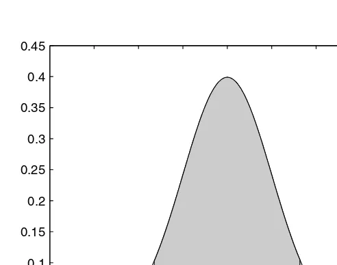
FFFFIIIIGUGUGUGURE 2.RE 2.RE 2.RE 2.2222
This shows the probability density function on the left with the associated cumulative distribution function on the right. Notice that the cumulative distribution function takes on values between 0 and 1.
0≤F x( )≤1
−4 −2 0 2 4
0 0.1 0.2 0.3 0.4
X
f(x)
−4 −2 0 2 4
0 0.2 0.4 0.6 0.8 1
X
F(x)
CDF
x1, ,x2 …
f x( )i = P X( = xi); i = 1 2, ,…
F a( ) f xi( ); xi≤a
∑
Axioms of
Axioms of
Axioms of
Axioms of PPPPrrrroba
oba
oba
obabbbbiiiilitlitlitlityyyy
Probabilities follow certain axioms that can be useful in computational statis-tics. We let S represent the sample space of an experiment and E represent some event that is a subset of S.
AXIOM 1
The probability of event E must be between 0 and 1: .
AXIOM 2
.
AXIOM 3
For mutually exclusive events, ,
.
Axiom 1 has been discussed before and simply states that a probability must be between 0 and 1. Axiom 2 says that an outcome from our experiment must occur, and the probability that the outcome is in the sample space is 1. Axiom 3 enables us to calculate the probability that at least one of the mutu-ally exclusive events occurs by summing the individual proba-bilities.
2.3 Conditional Probability and Independence
Conditional P
Conditional P
Conditional P
Conditional Prrrrob
ob
ob
obaaaabbbbiiiility
lity
lity
lity
Conditional probability is an important concept. It is used to define indepen-dent events and enables us to revise our degree of belief given that another event has occurred. Conditional probability arises in situations where we need to calculate a probability based on some partial information concerning the experiment.
The conditional probability of event E given event F is defined as follows: 0≤P E( )≤1
P S( ) = 1
E1,E2,…,Ek
P E( 1∪E2∪…∪Ek) P Ei( ) i=1
k
∑
=CONDITIONAL PROBABILITY
. (2.5)
Here represents the joint probability that both E and F occur together and is the probability that event F occurs. We can rearrange Equation 2.5 to get the following rule:
MULTIPLICATION RULE
. (2.6)
Ind Ind Ind
Indeeeependpendpendeeeencepend ncencence
Often we can assume that the occurrence of one event does not affect whether or not some other event happens. For example, say a couple would like to have two children, and their first child is a boy. The gender of their second child does not depend on the gender of the first child. Thus, the fact that we know they have a boy already does not change the probability that the sec-ond child is a boy. Similarly, we can sometimes assume that the value we observe for a random variable is not affected by the observed value of other random variables.
These types of events and random variables are called independent. If events are independent, then knowing that one event has occurred does not change our degree of belief or the likelihood that the other event occurs. If random variables are independent, then the observed value of one random variable does not affect the observed value of another.
In general, the conditional probability is not equal to . In these cases, the events are called dependent. Sometimes we can assume indepen-dence based on the situation or the experiment, which was the case with our example above. However, to show independence mathematically, we must use the following definition.
INDEPENDENT EVENTS
Two events E and F are said to be independent if and only if any of the following is true:
(2.7) P E F( ) P E( ∩F)
P F( )
---; P F( )>0 =
P E( ∩F) P F( )
P E( ∩F) = P F( )P E F( )
P E F( ) P E( )
Note that if events E and F are independent, then the Multiplication Rule in Equation 2.6 becomes
,
which means that we simply multiply the individual probabilities for each event together. This can be extended to k events to give
, (2.8)
where events and (for all i and j, ) are independent.
BBBBaaaaye
ye
ye
yessss Th
Th
Theeeeoooorrrreeeemmmm
Th
Sometimes we start an analysis with an initial degree of belief that an event will occur. Later on, we might obtain some additional information about the event that would change our belief about the probability that the event will occur. The initial probability is called a prior probability. Using the new information, we can update the prior probability using Bayes’ Theorem to obtain the posterior probability.
The experiment of recording piston ring failure in compressors is an exam-ple of where Bayes’ Theorem might be used, and we derive Bayes’ Theorem using this example. Suppose our piston rings are purchased from two manu-facturers: 60% from manufacturer A and 40% from manufacturer B.
Let denote the event that a part comes from manufacturer A, and represent the event that a piston ring comes from manufacturer B. If we select a part at random from our supply of piston rings, we would assign probabil-ities to these events as follows:
These are our prior probabilities that the piston rings are from the individual manufacturers.
Say we are interested in knowing the probability that a piston ring that sub-sequently failed came from manufacturer A. This would be the posterior probability that it came from manufacturer A, given that the piston ring failed. The additional information we have about the piston ring is that it failed, and we use this to update our degree of belief that it came from man-ufacturer A.
P E( ∩F) = P F( )P E( )
P E( 1∩E2∩…∩Ek) P Ei( ) i=1
k
∏
=Ei Ej i≠j
MA MB
Bayes’ Theorem can be derived from the definition of conditional probabil-ity (Equation 2.5). Writing this in terms of our events, we are interested in the following probability:
, (2.9)
where represents the posterior probability that the part came from manufacturer A, and F is the event that the piston ring failed. Using the Mul-tiplication Rule (Equation 2.6), we can write the numerator of Equation 2.9 in terms of event F and our prior probability that the part came from manufac-turer A, as follows
. (2.10)
The next step is to find . The only way that a piston ring will fail is if: 1) it failed and it came from manufacturer A or 2) it failed and it came from manufacturer B. Thus, using the third axiom of probability, we can write
.
Applying the Multiplication Rule as before, we have
. (2.11)
Substituting this for in Equation 2.10, we write the posterior probability as
. (2.12)
Note that we need to find the probabilities and . These are the probabilities that a piston ring will fail given it came from the correspond-ing manufacturer. These must be estimated in some way uscorrespond-ing available information (e.g., past failures). When we revisit Bayes’ Theorem in the con-text of statistical pattern recognition (Chapter 9), these are the probabilities that are estimated to construct a certain type of classifier.
Equation 2.12 is Bayes’ Theorem for a situation where only two outcomes are possible. In general, Bayes’ Theorem can be written for any number of mutually exclusive events, , whose union makes up the entire sam-ple space. This is given below.
BAYES’ THEOREM
. (2.13)
2.4 Expectation
Expected values and variances are important concepts in statistics. They are used to describe distributions, to evaluate the performance of estimators, to obtain test statistics in hypothesis testing, and many other applications.
Me Me Me
Meaaaannnn aaaandndndnd VVVVarianceariancearianceariance
The mean or expected value of a random variable is defined using the proba-bility density (mass) function. It provides a measure of central tendency of the distribution. If we observe many values of the random variable and take the average of them, we would expect that value to be close to the mean. The expected value is defined below for the discrete case.
EXPECTED VALUE - DISCRETE RANDOM VARIABLES
. (2.14)
We see from the definition that the expected value is a sum of all possible values of the random variable where each one is weighted by the probability that X will take on that value.
The variance of a discrete random variable is given by the following defi-nition.
VARIANCE - DISCRETE RANDOM VARIABLES
For ,
. (2.15)
P Ei( F) P Ei( )P F Ei( )
P E( )1 P F E( 1) …+ +P Ek( )P F Ek( ) ---=
µ E X[ ] xif xi( ) i=1
∞
∑
= =
µ ∞<
σ2
V X( ) E X( –µ)2
[ ] (xi–µ)2 f xi( ) i=1
∞
∑
From Equation 2.15, we see that the variance is the sum of the squared dis-tances, each one weighted by the probability that . Variance is a mea-sure of dispersion in the distribution. If a random variable has a large variance, then an observed value of the random variable is more likely to be far from the mean µ. The standard deviation is the square root of the vari-ance.
The mean and variance for continuous random variables are defined simi-larly, with the summation replaced by an integral. The mean and variance of a continuous random variable are given below.
EXPECTED VALUE - CONTINUOUS RANDOM VARIABLES
. (2.16)
VARIANCE - CONTINUOUS RANDOM VARIABLES
For ,
. (2.17)
We note that Equation 2.17 can also be written as
.
Other expected values that are of interest in statistics are the moments of a random variable. These are the expectation of powers of the random variable. In general, we define the r-th moment as
, (2.18)
and the r-th central moment as
SSSSkkkkeeeewwwwnnnnesesesesssss
The third central moment is often called a measure of asymmetry or skew-ness in the distribution. The uniform and the normal distribution are exam-ples of symmetric distributions. The gamma and the exponential are examples of skewed or asymmetric distributions. The following ratio is called the coefficient of skewness, which is often used to measure this char-acteristic:
. (2.20)
Distributions that are skewed to the left will have a negative coefficient of skewness, and distributions that are skewed to the right will have a positive value [Hogg and Craig, 1978]. The coefficient of skewness is zero for symmet-ric distributions. However, a coefficient of skewness equal to zero does not mean that the distribution must be symmetric.
Kurtosi Kurtosi Kurtosi Kurtosissss
Skewness is one way to measure a type of departure from normality. Kurtosis measures a different type of departure from normality by indicating the extent of the peak (or the degree of flatness near its center) in a distribution. The coefficient of kurtosis is given by the following ratio:
. (2.21)
We see that this is the ratio of the fourth central moment divided by the square of the variance. If the distribution is normal, then this ratio is equal to 3. A ratio greater than 3 indicates more values in the neighborhood of the mean (is more peaked than the normal distribution). If the ratio is less than 3, then it is an indication that the curve is flatter than the normal.
Sometimes the coefficient of excess kurtosis is used as a measure of kurto-sis. This is given by
. (2.22)
In this case, distributions that are more peaked than the normal correspond to a positive value of , and those with a flatter top have a negative coeffi-cient of excess kurtosis.
2.5 Common Distributions
In this section, we provide a review of some useful probability distributions and briefly describe some applications to modeling data. Most of these dis-tributions are used in later chapters, so we take this opportunity to define them and to fix our notation. We first cover two important discrete distribu-tions: the binomial and the Poisson. These are followed by several continuous distributions: the uniform, the normal, the exponential, the gamma, the chi-square, the Weibull, the beta and the multivariate normal.
Binomia
Binomia
Binomia
Binomiallll
Let’s say that we have an experiment, whose outcome can be labeled as a ‘success’ or a ‘failure’. If we let denote a successful outcome and represent a failure, then we can write the probability mass function as
(2.23)
where p represents the probability of a successful outcome. A random vari-able that follows the probability mass function in Equation 2.23 for
is called a Bernoulli random variable.
Now suppose we repeat this experiment for n trials, where each trial is independent (the outcome from one trial does not influence the outcome of another) and results in a success with probability p. If X denotes the number of successes in these n trials, then X follows the binomial distribution with parameters (n, p). Examples of binomial distributions with different parame-ters are shown in Figure 2.3.
To calculate a binomial probability, we use the following formula:
. (2.24)
The mean and variance of a binomial distribution are given by
and
X = 1
X = 0
f( )0 = P X( =0) = 1–p, f( )1 = P X( =1) = p,
0< <p 1
f x n( ; ,p) P X( =x) n x px
1–p ( )n–x
x
; 0 1, ,…,n
= = =
E X[ ] = np,
Some examples where the results of an experiment can be modeled by a bino-mial random variable are:
• A drug has probability 0.90 of curing a disease. It is administered to 100 patients, where the outcome for each patient is either cured or not cured. If X is the number of patients cured, then X is a binomial random variable with parameters (100, 0.90).
• The National Institute of Mental Health estimates that there is a 20% chance that an adult American suffers from a psychiatric dis-order. Fifty adult Americans are randomly selected. If we let X represent the number who have a psychiatric disorder, then X takes on values according to the binomial distribution with parameters (50, 0.20).
• A manufacturer of computer chips finds that on the average 5% are defective. To monitor the manufacturing process, they take a random sample of size 75. If the sample contains more than five defective chips, then the process is stopped. The binomial distri-bution with parameters (75, 0.05) can be used to model the random variable X, where X represents the number of defective chips.
FFFFIIIIGUGUGUGURE 2.RE 2.RE 2.3333RE 2.
Examples of the binomial distribution for different success probabilities.
0 1 2 3 4 5 6 0
0.05 0.1 0.15 0.2 0.25 0.3 0.35 0.4
n = 6, p = 0.3
X
0 1 2 3 4 5 6 0
0.05 0.1 0.15 0.2 0.25 0.3 0.35 0.4
n = 6, p = 0.7
Example 2.1
Suppose there is a 20% chance that an adult American suffers from a psychi-atric disorder. We randomly sample 25 adult Americans. If we let X represent the number of people who have a psychiatric disorder, then X is a binomial random variable with parameters . We are interested in the proba-bility that at most 3 of the selected people have such a disorder. We can use the MATLAB Statistics Toolbox function binocdf to determine , as follows:
prob = binocdf(3,25,0.2);
We could also sum up the individual values of the probability mass function
from to :
prob2 = sum(binopdf(0:3,25,0.2));
Both of these commands return a probability of 0.234. We now show how to generate the binomial distributions shown in Figure 2.3.
% Get the values for the domain, x. x = 0:6;
% Get the values of the probability mass function. % First for n = 6, p = 0.3:
pdf1 = binopdf(x,6,0.3); % Now for n = 6, p = 0.7: pdf2 = binopdf(x,6,0.7);
Now we have the values for the probability mass function (or the heights of the bars). The plots are obtained using the following code.
% Do the plots.
subplot(1,2,1),bar(x,pdf1,1,'w') title(' n = 6, p = 0.3')
xlabel('X'),ylabel('f(X)') axis square
subplot(1,2,2),bar(x,pdf2,1,'w') title(' n = 6, p = 0.7')
xlabel('X'),ylabel('f(X)') axis square
PPPPooooiiiisssssososonnnnso
A random variable X is a Poisson random variable with parameter , , if it follows the probability mass function given by
(2.25) 25 0.20,
( )
P X( ≤3)
X = 0 X = 3
λ λ>0
f x( ;λ) P X( = x) e–λλ
x
x!
---; x 0 1, ,…
The expected value and variance of a Poisson random variable are both λ, thus,
,
and
.
The Poisson distribution can be used in many applications. Examples of sit-uations where a discrete random variable might follow a Poisson distribution are:
• the number of typographical errors on a page,
• the number of vacancies in a company during a month, or • the number of defects in a length of wire.
The Poisson distribution is often used to approximate the binomial. When n is large and p is small (so is moderate), then the number of successes occurring can be approximated by the Poisson random variable with param-eter .
The Poisson distribution is also appropriate for some applications where events occur at points in time or space. We see it used in this context in Chap-ter 12, where we look at modeling spatial point patterns. Some other exam-ples include the arrival of jobs at a business, the arrival of aircraft on a runway, and the breakdown of machines at a manufacturing plant. The num-ber of events in these applications can be described by a Poisson process.
Let , , represent the number of events that occur in the time inter-val . For each interval , is a random variable that can take on values . If the following conditions are satisfied, then the counting process { , } is said to be a Poisson process with mean rate [Ross, 2000]:
1. .
2. The process has independent increments.
3. The number of events in an interval of length t follows a Poisson distribution with mean . Thus, for , ,
. (2.26)
From the third condition, we know that the process has stationary incre-ments. This means that the distribution of the number of events in an interval depends only on the length of the interval and not on the starting point. The
second condition specifies that the number of events in one interval does not affect the number of events in other intervals. The first condition states that the counting starts at time . The expected value of is given by
.
Example 2.2
In preparing this text, we executed the spell check command, and the editor reviewed the manuscript for typographical errors. In spite of this, some mis-takes might be present. Assume that the number of typographical errors per page follows the Poisson distribution with parameter . We calculate the probability that a page will have at least two errors as follows:
.
We can get this probability using the MATLAB Statistics Toolbox function poisscdf. Note that is the Poisson cumulative distri-bution function for (see Equation 2.4), which is why we use 1 as the argument to poisscdf.
prob = 1-poisscdf(1,0.25);
Example 2.3
Suppose that accidents at a certain intersection occur in a manner that satis-fies the conditions for a Poisson process with a rate of 2 per week ( ). What is the probability that at most 3 accidents will occur during the next 2 weeks? Using Equation 2.26, we have
.
Expanding this out yields
.
UUUUnnnniiiifor
for
for
formmmm
Perhaps one of the most important distributions is the uniform distribution for continuous random variables. One reason is that the uniform (0, 1) distri-bution is used as the basis for simulating most random variables as we dis-cuss in Chapter 4.
A random variable that is uniformly distributed over the interval (a, b) fol-lows the probability density function given by
. (2.27)
The parameters for the uniform are the interval endpoints, a and b. The mean and variance of a uniform random variable are given by
,
and
.
The cumulative distribution function for a uniform random variable is
(2.28)
Example 2.4
In this example, we illustrate the uniform probability density function over the interval (0, 10), along with the corresponding cumulative distribution function. The MATLAB Statistics Toolbox functions unifpdf and unifcdf are used to get the desired functions over the interval.
% First get the domain over which we will % evaluate the functions.
x = -1:.1:11;
Plots of the functions are provided in Figure 2.4, where the probability den-sity function is shown in the left plot and the cumulative distribution on the right. These plots are constructed using the following MATLAB commands.
% Do the plots.
subplot(1,2,1),plot(x,pdf) title('PDF')
xlabel('X'),ylabel('f(X)') axis([-1 11 0 0.2])
axis square
subplot(1,2,2),plot(x,cdf) title('CDF')
xlabel('X'),ylabel('F(X)') axis([-1 11 0 1.1])
axis square
FFFFIIIIGUGUGUGURE 2.RE 2.RE 2.RE 2.4444
On the left is a plot of the probability density function for the uniform (0, 10). Note that the
height of the curve is given by . The corresponding cumulative
distribution function is shown on the right.
0 5 10
0 0.02 0.04 0.06 0.08 0.1 0.12 0.14 0.16 0.18 0.2
X
f(X)
0 5 10
0 0.2 0.4 0.6 0.8 1
CDF
X
F(X)
NNNNoooorrrrma
ma
ma
mallll
A well known distribution in statistics and engineering is the normal distri-bution. Also called the Gaussian distribution, it has a continuous probability density function given by
(2.29)
where The normal distribution is
com-pletely determined by its parameters ( and ), which are also the expected value and variance for a normal random variable. The notation
is used to indicate that a random variable X is normally distributed with mean and variance . Several normal distributions with different param-eters are shown in Figure 2.5.
Some special properties of the normal distribution are given here.
• The value of the probability density function approaches zero as x approaches positive and negative infinity.
• The probability density function is centered at the mean , and the maximum value of the function occurs at .
• The probability density function for the normal distribution is sym-metric about the mean .
The special case of a standard normal random variable is one whose mean is zero , and whose standard deviation is one . If X is normally distributed, then
(2.30)
is a standard normal random variable.
Traditionally, the cumulative distribution function of a standard normal random variable is denoted by
. (2.31)
The cumulative distribution function for a standard normal random vari-able can be calculated using the error function, denoted by erf. The relation-ship between these functions is given by
. (2.32)
The error function can be calculated in MATLAB using erf(x). The MATLAB Statistics Toolbox has a function called normcdf(x,mu,sigma) that will calculate the cumulative distribution function for values in x. Its use is illustrated in the example given below.
Example 2.5
Similar to the uniform distribution, the functions normpdf and normcdf are available in the MATLAB Statistics Toolbox for calculating the probability density function and cumulative distribution function for the normal. There is another special function called normspec that determines the probability that a random variable X assumes a value between two limits, where X is nor-mally distributed with mean and standard deviation This function also plots the normal density, where the area between the specified limits is shaded. The syntax is shown below.
FFFFIIIIGUGUGUGURE 2.5RE 2.5RE 2.5RE 2.5
% Set up the parameters for the normal distribution. mu = 5;
sigma = 2;
% Set up the upper and lower limits. These are in % the two element vector 'specs'.
specs = [2, 8];
prob = normspec(specs, mu, sigma);
The resulting plot is shown in Figure 2.6. Note that the default title and axes labels are shown, but these can be changed easily using the title, xla-bel, and ylabel functions. You can also obtain tail probabilities by using -Inf as the first element of specs to designate no lower limit or Inf as the second element to indicate no upper limit.
EEEExponxponxponxponeeeentntntntiiiiaaaallll
The exponential distribution can be used to model the amount of time until a specific event occurs or to model the time between independent events. Some examples where an exponential distribution could be used as the model are:
FFFFIIIIGUGUGUGURE 2.RE 2.RE 2.RE 2.6666
• the time until the computer locks up,
• the time between arrivals of telephone calls, or • the time until a part fails.
The exponential probability density function with parameter is
. (2.33)
The mean and variance of an exponential random variable are given by the following:
,
and
.
FFFFIIIIGUGUGUGURE 2.RE 2.RE 2.7777RE 2.
Exponential probability density functions for various values of .
λ
f x( ;λ) = λe–λx; x≥0; λ>0
E X[ ] 1 λ ---=
V X( ) 1 λ2 ---=
0 0.5 1 1.5 2 2.5 3
0 0.2 0.4 0.6 0.8 1 1.2 1.4 1.6 1.8 2
x
f(x)
Exponential Distribution
λ = 2
λ = 1
λ = 0.5