Digital Systems
Principles and Applications
Ronald J. Tocci
Monroe Community College
Neal S. Widmer
Purdue University
Gregory L. Moss
Purdue University
TENTH EDITION
Director of Development:Vern Anthony Editorial Assistant: Lara Dimmick Production Editor: Stephen C. Robb
Production Coordination:Peggy Hood, TechBooks/GTS Design Coordinator: Diane Y. Ernsberger
Cover Designer: Jason Moore Cover Art: Getty One
Production Manager: Matt Ottenweller Marketing Manager: Ben Leonard
This book was set in TimesEuropa Roman by TechBooks/GTSYork, PA Campus. It was printed and bound by Courier Kendallville, Inc. The cover was printed by Phoenix Color Corp.
MultiSIM®is a trademark of Electronics Workbench.
Altera is a trademark and service mark of Altera Corporation in the United States and other countries. Altera products are the intellectual property of Altera Corporation and are protected by copyright laws and one or more U.S. and foreign patents and patent ap-plications.
Copyright © 2007 by Pearson Education, Inc., Upper Saddle River, New Jersey 07458. Pearson Prentice Hall. All rights reserved. Printed in the United States of America. This publication is protected by Copyright and permission should be obtained from the pub-lisher prior to any prohibited reproduction, storage in a retrieval system, or transmission in any form or by any means, electronic, mechanical, photocopying, recording, or likewise. For information regarding permission(s), write to: Rights and Permissions Department.
Pearson Prentice Hall™is a trademark of Pearson Education, Inc. Pearson®is a registered trademark of Pearson plc
Prentice Hall®is a registered trademark of Pearson Education, Inc.
Pearson Education Ltd. Pearson Education Australia Pty. Limited Pearson Education Singapore, Pte. Ltd. Pearson Education North Asia Ltd. Pearson Education Canada, Ltd. Pearson Educación de Mexico, S.A. de C.V. Pearson Education—Japan Pearson Education Malaysia, Pte. Ltd. Pearson Education, Upper Saddle River,
New Jersey
To you, Cap, for loving me for so long; and for the million
and one ways you brighten the lives of everyone you touch.
—RJT
To my wife, Kris, and our children, John, Brad, Blake,
Matt, and Katie: the lenders of their rights to my time and
attention that this revision might be accomplished.
—NSW
To my family, Marita, David, and Ryan.
vii
P R E F A C E
This book is a comprehensive study of the principles and techniques of mod-ern digital systems. It teaches the fundamental principles of digital systems and covers thoroughly both traditional and modern methods of applying dig-ital design and development techniques, including how to manage a systems-level project. The book is intended for use in two- and four-year programs in technology, engineering, and computer science. Although a background in basic electronics is helpful, most of the material requires no electronics training. Portions of the text that use electronics concepts can be skipped without adversely affecting the comprehension of the logic principles.
General Improvements
The tenth edition of Digital Systems reflects the authors’ views of the direction of modern digital electronics. In industry today, we see the impor-tance of getting a product to market very quickly. The use of modern design tools, CPLDs, and FPGAs allows engineers to progress from concept to func-tional silicon very quickly. Microcontrollers have taken over many applica-tions that once were implemented by digital circuits, and DSP has been used to replace many analog circuits. It is amazing that microcontrollers, DSP, and all the necessary glue logic can now be consolidated onto a single FPGA using a hardware description language with advanced development tools. Today’s students must be exposed to these modern tools, even in an introductory course. It is every educator’s responsibility to find the best way to prepare graduates for the work they will encounter in their profes-sional lives.
the curriculum. From an educational standpoint, however, these small ICs do offer a way to study simple digital circuits, and the wiring of circuits using breadboards is a valuable pedagogic exercise. They help to solidify concepts such as binary inputs and outputs, physical device operation, and practical limitations, using a very simple platform. Consequently, we have chosen to continue to introduce the conceptual descriptions of digital circuits and to offer examples using conventional standard logic parts. For instructors who continue to teach the fundamentals using SSI and MSI circuits, this edition retains those qualities that have made the text so widely accepted in the past. Many hardware design tools even provide an easy-to-use design entry technique that will employ the functionality of conventional standard parts with the flexibility of programmable logic devices. A digital design can be described using a schematic drawing with pre-created building blocks that are equivalent to conventional standard parts, which can be compiled and then programmed directly into a target PLD with the added capability of easily simulating the design within the same development tool.
We believe that graduates will actually apply the concepts presented in this book using higher-level description methods and more complex program-mable devices. The major shift in the field is a greater need to understand the description methods, rather than focusing on the architecture of an actual de-vice. Software tools have evolved to the point where there is little need for con-cern about the inner workings of the hardware but much more need to focus on what goes in, what comes out, and how the designer can describe what the device is supposed to do. We also believe that graduates will be involved with projects using state-of-the-art design tools and hardware solutions.
This book offers a strategic advantage for teaching the vital new topic of hardware description languages to beginners in the digital field. VHDL is undisputedly an industry standard language at this time, but it is also very complex and has a steep learning curve. Beginning students are often dis-couraged by the rigorous requirements of various data types, and they strug-gle with understanding edge-triggered events in VHDL. Fortunately, Altera offers AHDL, a less demanding language that uses the same basic concepts as VHDL but is much easier for beginners to master. So, instructors can opt to use AHDL to teach introductory students or VHDL for more advanced classes. This edition offers more than 40 AHDL examples, more than 40 VHDL examples, and many examples of simulation testing. All of these design files are available on the enclosed CD-ROM.
PREFACE
ix
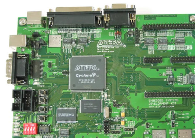
newer board from Altera is called the DE2 board (see Figure P-2), which has a powerful new 672-pin Cyclone II FPGA and a number of basic features such as switches, LEDs, and displays as well as many additional features for more advanced projects. More development boards are entering the market every year, and many are becoming very affordable. These boards, along with pow-erful educational software, offer an excellent way to teach and demonstrate the practical implementation of the concepts presented in this text.
The most significant improvements in the tenth edition are found in Chap-ter 7. Although asynchronous (ripple) counChap-ters provide a good introduction to sequential circuits, the real world uses synchronous counter circuits. Chapter 7 and subsequent examples have been rewritten to emphasize synchronous counter ICs and include techniques for analysis, cascading, and using HDL to describe them. A section has also been added to improve the coverage of state machines and the HDL features used to describe them. Other improvements include analysis techniques for combinational circuits, expanded coverage of 555 timer applications, and better coverage of signed binary numbers.
FIGURE P-1 Altera’s UP3 development board.
Our approach to HDL and PLDs gives instructors several options:
1. The HDL material can be skipped entirely without affecting the continuity of the text.
2. HDL can be taught as a separate topic by skipping the material initially and then going back to the last sections of Chapters 3, 4, 5, 6, 7, and 9 and then covering Chapter 10.
3. HDL and the use of PLDs can be covered as the course unfolds— chapter by chapter—and woven into the fabric of the lecture/ lab experience.
Among all specific hardware description languages, VHDL is clearly the industry standard and is most likely to be used by graduates in their careers. We have always felt that it is a bold proposition, however, to try to teach VHDL in an introductory course. The nature of the syntax, the subtle distinctions in object types, and the higher levels of abstraction can pose obstacles for a beginner. For this reason, we have included Altera’s AHDL as the recom-mended introductory language for freshman courses. We have also included VHDL as the recommended language for more advanced classes or introduc-tory courses offered to more mature students. We do not recommend trying to cover both languages in the same course. Sections of the text that cover the specifics of a language are clearly designated with a color bar in the margin. The HDL code figures are set in a color to match the color-coded text expla-nation.The reader can focus only on the language of his or her choice and skip the other. Obviously, we have attempted to appeal to the diverse interests of our market, but we believe we have created a book that can be used in multi-ple courses and will serve as an excellent reference after graduation.
Chapter Organization
It is a rare instructor who uses the chapters of a textbook in the sequence in which they are presented. This book was written so that, for the most part, each chapter builds on previous material, but it is possible to alter the chap-ter sequence somewhat. The first part of Chapchap-ter 6 (arithmetic operations) can be covered right after Chapter 2 (number systems), although this will lead to a long interval before the arithmetic circuits of Chapter 6 are encountered. Much of the material in Chapter 8 (IC characteristics) can be covered earlier (e.g., after Chapter 4 or 5) without creating any serious problems.
This book can be used either in a one-term course or in a two-term se-quence. In a one-term course, limits on available class hours might require omitting some topics. Obviously, the choice of deletions will depend on fac-tors such as program or course objectives and student background. A list of sections and chapters that can be deleted with minimal disruption follows:
■ Chapter 1: All ■ Chapter 2: Section 6 ■ Chapter 3: Sections 15–20 ■ Chapter 4: Sections 7, 10–13 ■ Chapter 5: Sections 3, 23–27
PREFACE
xi
FIGURE P-3 Letters denote categories of problems, and asterisks indicate that corresponding solutions are provided at the end of the text.
■ Chapter 9: Sections 5, 9, 15–20 ■ Chapter 10: All
■ Chapter 11: Sections 7, 14–17 ■ Chapter 12: Sections 17–21 ■ Chapter 13: All
PROBLEM SETS This edition includes six categories of problems: basic (B), challenging (C), troubleshooting (T), new (N), design (D), and HDL (H). Undesignated problems are considered to be of intermediate difficulty, be-tween basic and challenging. Problems for which solutions are printed in the back of the text or on the enclosed CD-ROM are marked with an asterisk (see Figure P-3).
PROJECT MANAGEMENT AND SYSTEM-LEVEL DESIGN Several real-world examples are included in Chapter 10 to describe the techniques used to manage projects. These applications are generally familiar to most stu-dents studying electronics, and the primary example of a digital clock is fa-miliar to everyone. Many texts talk about top-down design, but this text demonstrates the key features of this approach and how to use the modern tools to accomplish it.
DATA SHEETS The CD-ROM containing Texas Instruments data sheets that accompanied the ninth edition has been removed. The information that was included on this CD-ROM is now readily available online.
for students. All figures in the text that have a corresponding simulation file on the CD-ROM are identified by the icon shown in Figure P-4.
IC TECHNOLOGY This new edition continues the practice begun with the last three editions of giving more prominence to CMOS as the principal IC technology in small- and medium-scale integration applications. This depth of coverage has been accomplished while retaining the substantial coverage of TTL logic.
Specific Changes
The major changes in the topical coverage are listed here.
■ Chapter 1. Many explanations covering digital/analog issues have been
updated and improved.
■ Chapter 2. The octal number system has been removed and the Gray
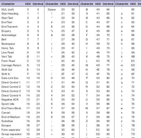
code has been added. A complete standard ASCII code table has been in-cluded, along with new examples that relate ASCII characters, hex rep-resentation, and computer object code transfer files. New material on framing ASCII characters for asynchronous data transfer has also been added.
■ Chapter 3. Along with some new practical examples of logic functions,
the major improvement in Chapter 3 is a new analysis technique using tables that evaluate intermediate points in the logic circuit.
■ Chapter 4. Very few changes were necessary in Chapter 4.
■ Chapter 5. A new section covers digital pulses and associated definitions
such as pulse width, period, rise time, and fall time. The terminology used for latch circuit inputs has been changed from Clear to Reset in order to be compatible with Altera component descriptions. The definition of a master/slave flip-flop has been removed as well. The discussion of Schmitt trigger applications has been improved to emphasize their role in eliminating the effects of noise. The inner workings of the 555 timer are now explained, and some improved timing circuits are proposed that make the device more versatile. The HDL coverage of SR and D latches has been rewritten to use a more intuitive behavioral description, and the coverage of counters has been modified to focus on structural tech-niques to interconnect flip-flop blocks.
■ Chapter 6. Signed numbers are covered in more detail in this edition,
particularly regarding sign extension in 2’s complement numbers and arithmetic overflow. A new calculator hint simplifies negation of binary numbers represented in hex. A number circle model is used to compare FIGURE P-4 The icon
signed and unsigned number formats and help students to visualize add/subtract operation using both.
■ Chapter 7. This chapter has been heavily revised to emphasize synchro-nous counter circuits. Simple ripple counters are still introduced to pro-vide a basic understanding of the concept of counting and asynchronous cascading. After examining the limitations of ripple counters in Section 2, synchronous counters are introduced in Section 3 and used in all subse-quent examples throughout the text. The IC counters presented are the 74160, ’161, ’162, and ’163. These common devices offer an excellent assort-ment of features that teach the difference between synchronous and asyn-chronous control inputs and cascading techniques. The 74190 and ’191 are used as an example of a synchronous up/down counter IC, further rein-forcing the techniques required for synchronous cascading. A new section is devoted to analysis techniques for synchronous circuits using JK and D flip-flops. Synchronous design techniques now also include the use of D flip-flop registers that best represent the way sequential circuits are plemented in modern PLD technology. The HDL sections have been im-proved to demonstrate the implementation of synchronous/asynchronous loading, clearing, and cascading. A new emphasis is placed on simulation and testing of HDL modules. State machines are now presented as a topic, the traditional Mealy and Moore models are defined, and a new traffic light control system is presented as an example. Minor improvements have been made in the second half of Chapter 7 also. All of the problems at the end of Chapter 7 have been rewritten to reinforce the concepts.
■ Chapter 8. This chapter remains a very technical description of the tech-nology available in standard logic families and digital components. The mixed-voltage interfacing sections have been improved to cover low-voltage technology. The latest Texas Instruments life-cycle curve shows the history and current position of various logic series between intro-duction and obsolescence. Low-voltage differential signaling (LVDS) is introduced as well.
■ Chapter 9. The many different building blocks of digital systems are still covered in this chapter and demonstrated using HDL. Many other HDL techniques, such as tristate outputs and various HDL control structures, are also introduced. A 74ALS148 is described as another example of an encoder. The examples of systems that use counters have all been updated to synchronous operation. The serial transmission system using MUX and DEMUX is particularly improved. The technique of using a MUX to implement SOP expressions has been explained in a more structured way as an independent study exercise in the end-of-the-chapter problems.
■ Chapter 10. Chapter 10, which was new to the ninth edition, has re-mained essentially unchanged.
■ Chapter 11. The material on bipolar DACs has been improved, and an ex-ample of using DACs as a digital amplitude control for analog waveforms is presented. The more common A / D converter accuracy specification in the form of ⫹/⫺LSB is explained in this edition.
■ Chapter 12. Minor improvements were made to this chapter to consolidate and compress some of the material on older technologies of memory such as UV EPROM. Flash technology is still introduced using a first-generation example, but the more recent improvements, as well as some of the appli-cations of flash technology in modern consumer devices, are described.
■ Chapter 13. This chapter, which was new to the ninth edition, has been updated to introduce the new Cyclone family of PLDs.
Retained Features
This edition retains all of the features that made the previous editions so widely accepted. It utilizes a block diagram approach to teach the basic logic operations without confusing the reader with the details of internal operation. All but the most basic electrical characteristics of the logic ICs are withheld until the reader has a firm understanding of logic principles. In Chapter 8, the reader is introduced to the internal IC circuitry. At that point, the reader can interpret a logic block’s input and output characteristics and “fit” it properly into a complete system.
The treatment of each new topic or device typically follows these steps: the principle of operation is introduced; thoroughly explained examples and applications are presented, often using actual ICs; short review questions are posed at the end of the section; and finally, in-depth problems are available at the end of the chapter. These problems, ranging from simple to complex, provide instructors with a wide choice of student assignments. These prob-lems are often intended to reinforce the material without simply repeating the principles. They require students to demonstrate comprehension of the principles by applying them to different situations. This approach also helps students to develop confidence and expand their knowledge of the material. The material on PLDs and HDLs is distributed throughout the text, with examples that emphasize key features in each application. These topics ap-pear at the end of each chapter, making it easy to relate each topic to the gen-eral discussion earlier in the chapter or to address the gengen-eral discussion separately from the PLD/HDL coverage.
The extensive troubleshooting coverage is spread over Chapters 4 through 12 and includes presentation of troubleshooting principles and techniques, case studies, 25 troubleshooting examples, and 60 realtroubleshooting prob-lems. When supplemented with hands-on lab exercises, this material can help foster the development of good troubleshooting skills.
The tenth edition offers more than 200 worked-out examples, more than 400 review questions, and more than 450 chapter problems/exercises. Some of these problems are applications that show how the logic devices presented in the chapter are used in a typical microcomputer system. Answers to a majority of the problems immediately follow the Glossary. The Glossary pro-vides concise definitions of all terms in the text that have been highlighted in boldface type.
An IC index is provided at the back of the book to help readers locate eas-ily material on any IC cited or used in the text. The back endsheets provide tables of the most often used Boolean algebra theorems, logic gate summaries, and flip-flop truth tables for quick reference when doing problems or work-ing in the lab.
Supplements
An extensive complement of teaching and learning tools has been developed to accompany this textbook. Each component provides a unique function, and each can be used independently or in conjunction with the others.
CD-ROM A CD-ROM is packaged with each copy of the text. It contains the following material:
digital systems that has been used for many years and is still supported by Altera. Students can use it to write, compile, and simulate their de-signs at home before going to the lab. They can use the same software to program and test an Altera CPLD.
■ Quartus II Web Version software from Altera.This is the latest
develop-ment system software from Altera, which offers more advanced features and supports new PLD devices such as the Cyclone family of FPGAs, found on many of the newest educational boards.
■ Tutorials. Gregory Moss has developed tutorials that have been used
successfully for several years to teach introductory students how to use Altera MAX⫹PLUS II software. These tutorials are available in PDF and PPT (Microsoft®PowerPoint®presentation) formats and have been adapted to teach Quartus II as well. With the help of these tutorials, any-one can learn to modify and test all the examples presented in this text, as well as develop his or her own designs.
■ Design files from the textbook figures.More than 40 design files in each
language are presented in figures throughout the text. Students can load these into the Altera software and test them.
■ Solutions to selected problems: HDL design files.A few of the
end-of-chapter problem solutions are available to students. (All of the HDL solutions are available to instructors in the Instructor’s Resource Manual.)
Solutions for Chapter 7 problems include some large graphic and HDL files that are not published in the back of the book but are available on the enclosed CD-ROM.
■ Circuits from the text rendered in Multisim®. Students can open and
work interactively with approximately 100 circuits to increase their un-derstanding of concepts and prepare for laboratory activities. The Multisim circuit files are provided for use by anyone who has Multisim software. Anyone who does not have Multisim software and wishes to purchase it in order to use the circuit files may do so by ordering it from www.prenhall.com/ewb.
■ Supplemental material introducing microprocessors and
microcon-trollers.For the flexibility to serve the diverse needs of the many differ-ent schools, an introduction to this topic is presdiffer-ented as a convenidiffer-ent bridge between a digital systems course and an introduction to micro-processors/microcontrollers course.
STUDENT RESOURCES
■ Lab Manual: A Design Approach. This lab manual, written by Gregory
Moss, contains topical units with lab projects that emphasize simulation and design. It utilizes the Altera MAX⫹PLUS II or Quartus II software in its programmable logic exercises and features both schematic capture and hardware description language techniques. The new edition con-tains many new projects and examples. (ISBN 0-13-188138-8)
■ Lab Manual: A Troubleshooting Approach.This manual, written by Jim
DeLoach and Frank Ambrosio, is presented with an analysis and trou-bleshooting approach and is fully updated for this edition of the text. (ISBN 0-13-188136-1)
■ Companion Website (www.prenhall.com/tocci).This site offers students a
free online study guide with which they can review the material learned in the text and check their understanding of key topics.
INSTRUCTOR RESOURCES
■ Instructor’s Resource Manual.This manual contains worked-out solutions for all end-of-chapter problems in this textbook. (ISBN 0-13-172665-X)
■ Lab Solutions Manual.Worked-out lab results for both lab manuals are featured in this manual. (ISBN 0-13-172664-1)
■ PowerPoint®presentations.Figures from the text, in addition to Lecture Notes for each chapter, are available on CD-ROM. (ISBN 0-13-172667-6)
■ TestGen.A computerized test bank is available on CD-ROM. (ISBN 0-13-172666-8)
To access supplementary materials online, instructors need to request an instructor access code. Go to www.prenhall.com,click the Instructor Resource Centerlink, and then click Register Todayfor an instructor access code.Within 48 hours after registering, you will receive a confirming e-mail including an instructor access code. When you have received your code, go to the site and log on for full instructions on downloading the materials you wish to use.
ACKNOWLEDGMENTS
We are grateful to all those who evaluated the ninth edition and provided answers to an extensive questionnaire: Ali Khabari, Wentworth Institute of Technology; Al Knebel, Monroe Community College; Rex Fisher, Brigham Young University; Alan Niemi, LeTourneau University; and Roger Sash, Uni-versity of Nebraska. Their comments, critiques, and suggestions were given serious consideration and were invaluable in determining the final form of the tenth edition.
We also are greatly indebted to Professor Frank Ambrosio, Monroe Com-munity College, for his usual high-quality work on the indexes and the Ins-tructor’s Resource Manual; and Professor Thomas L. Robertson, Purdue University, for providing his magnetic levitation system as an example; and Professors Russ Aubrey and Gene Harding, Purdue University, for their tech-nical review of topics and many suggestions for improvements. We appreci-ate the cooperation of Mike Phipps and the Altera Corporation for their support in granting permission to use their software package and their fig-ures from technical publications.
A writing project of this magnitude requires conscientious and profes-sional editorial support, and Prentice Hall came through again in typical fashion. We thank the staffs at Prentice Hall and TechBooks/GTS for their help to make this publication a success.
And finally, we want to let our wives and our children know how much we appreciate their support and their understanding. We hope that we can even-tually make up for all the hours we spent away from them while we worked on this revision.
xvii
B R I E F C O N T E N T S
CHAPTER 1
Introductory Concepts
2
CHAPTER 2
Number Systems and Codes
24
CHAPTER 3
Describing Logic Circuits
54
CHAPTER 4
Combinational Logic Circuits
118
CHAPTER 5
Flip-Flops and Related Devices
208
CHAPTER 6
Digital Arithmetic: Operations and Circuits
296
CHAPTER 7
Counters and Registers
360
CHAPTER 8
Integrated-Circuit Logic Families
488
CHAPTER 9
MSI Logic Circuits
576
CHAPTER 10 Digital System Projects Using HDL
676
CHAPTER 11 Interfacing with the Analog World
718
CHAPTER 12 Memory Devices
786
CHAPTER 13 Programmable Logic Device Architectures
868
Glossary
898
Answers to Selected Problems
911
Index of ICs
919
xix
C O N T E N T S
CHAPTER 1
Introductory Concepts
2
1-1 Numerical Representations 4
1-2 Digital and Analog Systems 5
1-3 Digital Number Systems 10
1-4 Representing Binary Quantities 13
1-5 Digital Circuits/Logic Circuits 15
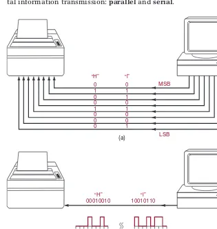
1-6 Parallel and Serial Transmission 17
1-7 Memory 18
1-8 Digital Computers 19
CHAPTER 2
Number Systems and Codes
24
2-1 Binary-to-Decimal Conversions 26
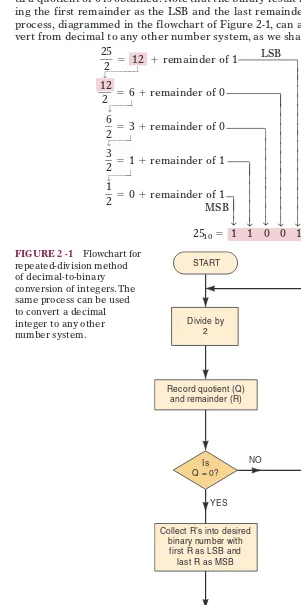
2-2 Decimal-to-Binary Conversions 26
2-3 Hexadecimal Number System 29
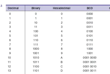
2-4 BCD Code 33
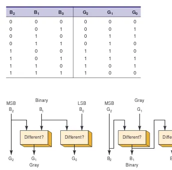
2-5 The Gray Code 35
2-6 Putting It All Together 37
2-7 The Byte, Nibble, and Word 37
2-8 Alphanumeric Codes 39
2-9 Parity Method for Error Detection 41
Chapter 3
Describing Logic Circuits
54
3-1 Boolean Constants and Variables 57
3-2 Truth Tables 57
3-3 OR Operation with OR Gates 58
3-4 AND Operation with AND Gates 62
3-5 NOT Operation 65
3-6 Describing Logic Circuits Algebraically 66
3-7 Evaluating Logic-Circuit Outputs 68
3-8 Implementing Circuits from Boolean Expressions 71
3-9 NOR Gates and NAND Gates 73
3-10 Boolean Theorems 76
3-11 DeMorgan’s Theorems 80
3-12 Universality of NAND Gates and NOR Gates 83
3-13 Alternate Logic-Gate Representations 86
3-14 Which Gate Representation to Use 89
3-15 IEEE/ANSI Standard Logic Symbols 95
3-16 Summary of Methods to Describe Logic Circuits 96
3-17 Description Languages Versus Programming Languages 98
3-18 Implementing Logic Circuits with PLDs 100
3-19 HDL Format and Syntax 102
3-20 Intermediate Signals 105
Chapter 4
Combinational Logic Circuits
118
4-1 Sum-of-Products Form 120
4-2 Simplifying Logic Circuits 121
4-3 Algebraic Simplification 121
4-4 Designing Combinational Logic Circuits 127
4-5 Karnaugh Map Method 133
4-6 Exclusive-OR and Exclusive-NOR Circuits 144
4-7 Parity Generator and Checker 149
4-8 Enable/Disable Circuits 151
4-9 Basic Characteristics of Digital ICs 153
4-10 Troubleshooting Digital Systems 160
4-11 Internal Digital IC Faults 162
4-12 External Faults 166
4-13 Troubleshooting Case Study 168
4-14 Programmable Logic Devices 170
4-15 Representing Data in HDL 177
4-16 Truth Tables Using HDL 181
Chapter 5
Flip-Flops and Related Devices
208
5-1 NAND Gate Latch 211
5-2 NOR Gate Latch 216
5-3 Troubleshooting Case Study 219
5-4 Digital Pulses 220
5-5 Clock Signals and Clocked Flip-Flops 221
5-6 Clocked S-R Flip-Flop 224
5-7 Clocked J-K Flip-Flop 227
5-8 Clocked D Flip-Flop 230
5-9 DLatch (Transparent Latch) 232
5-10 Asynchronous Inputs 233
5-11 IEEE/ANSI Symbols 236
5-12 Flip-Flop Timing Considerations 238
5-13 Potential Timing Problem in FF Circuits 241
5-14 Flip-Flop Applications 243
5-15 Flip-Flop Synchronization 243
5-16 Detecting an Input Sequence 244
5-17 Data Storage and Transfer 245
5-18 Serial Data Transfer: Shift Registers 247
5-19 Frequency Division and Counting 250
5-20 Microcomputer Application 254
5-21 Schmitt-Trigger Devices 256
5-22 One-Shot (Monostable Multivibrator) 256
5-23 Clock Generator Circuits 260
5-24 Troubleshooting Flip-Flop Circuits 264
5-25 Sequential Circuits Using HDL 268
5-26 Edge-Triggered Devices 272
5-27 HDL Circuits with Multiple Components 277
Chapter 6
Digital Arithmetic:
Operations and Circuits
296
6-1 Binary Addition 298
6-2 Representing Signed Numbers 299
6-3 Addition in the 2’s-Complement System 306
6-4 Subtraction in the 2’s-Complement System 307
6-5 Multiplication of Binary Numbers 310
6-6 Binary Division 311
6-7 BCD Addition 312
6-8 Hexadecimal Arithmetic 314
6-9 Arithmetic Circuits 317
6-10 Parallel Binary Adder 318
6-11 Design of a Full Adder 320
6-12 Complete Parallel Adder with Registers 323
6-13 Carry Propagation 325
6-14 Integrated-Circuit Parallel Adder 326
6-15 2’s-Complement System 328
6-16 ALU Integrated Circuits 331
6-17 Troubleshooting Case Study 335
6-18 Using TTL Library Functions with HDL 337
6-19 Logical Operations on Bit Arrays 338
6-20 HDL Adders 340
6-21 Expanding the Bit Capacity of a Circuit 343
Chapter 7
Counters and Registers
360
7-1 Asynchronous (Ripple) Counters 362
7-2 Propagation Delay in Ripple Counters 365
7-3 Synchronous (Parallel) Counters 367
7-4 Counters with MOD Numbers <2N 370
7-5 Synchronous Down and Up/Down Counters 377
7-6 Presettable Counters 379
7-7 IC Synchronous Counters 380
7-8 Decoding a Counter 389
7-9 Analyzing Synchronous Counters 393
7-10 Synchronous Counter Design 396
7-11 Basic Counters Using HDLs 405
7-12 Full-Featured Counters in HDL 412
7-13 Wiring HDL Modules Together 417
7-14 State Machines 425
7-15 Integrated-Circuit Registers 437
7-16 Parallel In/Parallel Out—The 74ALS174/74HC174 437
7-17 Serial In/Serial Out—The 74ALS166/ 74HC166 439
7-18 Parallel In/Serial Out—The 74ALS165/74HC165 441
7-19 Serial In/Parallel Out—The 74ALS164/74HC164 443
7-20 Shift-Register Counters 445
7-21 Troubleshooting 450
7-22 HDL Registers 452
7-23 HDL Ring Counters 459
7-24 HDL One-Shots 461
Chapter 8
Integrated-Circuit Logic Families
488
8-1 Digital IC Terminology 490
8-2 The TTL Logic Family 498
8-3 TTL Data Sheets 502
8-5 TTL Loading and Fan-Out 509
8-6 Other TTL Characteristics 514
8-7 MOS Technology 518
8-8 Complementary MOS Logic 521
8-9 CMOS Series Characteristics 523
8-10 Low-Voltage Technology 530
8-11 Open-Collector/Open-Drain Outputs 533
8-12 Tristate (Three-State) Logic Outputs 538
8-13 High-Speed Bus Interface Logic 541
8-14 The ECL Digital IC Family 543
8-15 CMOS Transmission Gate (Bilateral Switch) 546
8-16 IC Interfacing 548
8-17 Mixed-Voltage Interfacing 553
8-18 Analog Voltage Comparators 554
8-19 Troubleshooting 556
Chapter 9
MSI Logic Circuits
576
9-1 Decoders 577
9-2 BCD-to-7-Segment Decoder/Drivers 584
9-3 Liquid-Crystal Displays 587
9-4 Encoders 591
9-5 Troubleshooting 597
9-6 Multiplexers (Data Selectors) 599
9-7 Multiplexer Applications 604
9-8 Demultiplexers (Data Distributors) 610
9-9 More Troubleshooting 617
9-10 Magnitude Comparator 621
9-11 Code Converters 624
9-12 Data Busing 628
9-13 The 74ALS173/HC173 Tristate Register 629
9-14 Data Bus Operation 632
9-15 Decoders Using HDL 638
9-16 The HDL 7-Segment Decoder/Driver 642
9-17 Encoders Using HDL 645
9-18 HDL Multiplexers and Demultiplexers 648
9-19 HDL Magnitude Comparators 652
9-20 HDL Code Converters 653
Chapter 10 Digital System Projects Using HDL
676
10-1 Small-Project Management 678
10-2 Stepper Motor Driver Project 679
10-3 Keypad Encoder Project 687
10-4 Digital Clock Project 693
10-5 Frequency Counter Project 710
Chapter 11 Interfacing with the Analog World
718
11-1 Review of Digital Versus Analog 719
11-2 Digital-to-Analog Conversion 721
11-3 D/A-Converter Circuitry 728
11-4 DAC Specifications 733
11-5 An Integrated-Circuit DAC 735
11-6 DAC Applications 736
11-7 Troubleshooting DACs 738
11-8 Analog-to-Digital Conversion 739
11-9 Digital-Ramp ADC 740
11-10 Data Acquisition 745
11-11 Successive-Approximation ADC 749
11-12 Flash ADCs 755
11-13 Other A/D Conversion Methods 757
11-14 Sample-and-Hold Circuits 761
11-15 Multiplexing 762
11-16 Digital Storage Oscilloscope 764
11-17 Digital Signal Processing (DSP) 765
Chapter 12 Memory Devices
784
12-1 Memory Terminology 786
12-2 General Memory Operation 790
12-3 CPU–Memory Connections 793
12-4 Read-Only Memories 795
12-5 ROM Architecture 796
12-6 ROM Timing 799
12-7 Types of ROMs 800
12-8 Flash Memory 808
12-9 ROM Applications 811
12-10 Semiconductor RAM 814
12-11 RAM Architecture 815
12-12 Static RAM (SRAM) 818
12-13 Dynamic RAM (DRAM) 823
12-14 Dynamic RAM Structure and Operation 824
12-15 DRAM Read/Write Cycles 829
12-16 DRAM Refreshing 831
12-17 DRAM Technology 834
12-18 Expanding Word Size and Capacity 836
12-20 Troubleshooting RAM Systems 847
12-21 Testing ROM 852
Chapter 13 Programmable Logic Device
Architectures
868
13-1 Digital Systems Family Tree 870
13-2 Fundamentals of PLD Circuitry 875
13-3 PLD Architectures 877
13-4 The GAL 16V8 (Generic Array Logic) 881
13-5 The Altera EPM7128S CPLD 885
13-6 The Altera FLEX10K Family 890
13-7 The Altera Cyclone Family 894
Glossary
898
Answers to Selected Problems
911
Index of ICs
919
Index
922
1-1 Numerical Representations 1-2 Digital and Analog Systems 1-3 Digital Number Systems 1-4 Representing Binary
Quantities
1-5 Digital Circuits/Logic Circuits
■
OUTLINE
I N T R O D U C T O R Y
C O N C E P T S
1-6 Parallel and Serial Transmission 1-7 Memory
3
■
OBJECTIVES
Upon completion of this chapter, you will be able to:
■ Distinguish between analog and digital representations.
■ Cite the advantages and drawbacks of digital techniques compared with analog.
■ Understand the need for analog-to-digital converters (ADCs) and digital-to-analog converters (DACs).
■ Recognize the basic characteristics of the binary number system. ■ Convert a binary number to its decimal equivalent.
■ Count in the binary number system. ■ Identify typical digital signals. ■ Identify a timing diagram.
■ State the differences between parallel and serial transmission. ■ Describe the property of memory.
■ Describe the major parts of a digital computer and understand their functions.
■ Distinguish among microcomputers, microprocessors, and microcontrollers.
■
INTRODUCTION
In today’s world, the term digitalhas become part of our everyday vocabu-lary because of the dramatic way that digital circuits and digital techniques have become so widely used in almost all areas of life: computers, automa-tion, robots, medical science and technology, transportaautoma-tion, telecommuni-cations, entertainment, space exploration, and on and on. You are about to begin an exciting educational journey in which you will discover the funda-mental principles, concepts, and operations that are common to all digital systems, from the simplest on/off switch to the most complex computer. If this book is successful, you should gain a deep understanding of how all digital systems work, and you should be able to apply this understanding to the analysis and troubleshooting of any digital system.
1-1
NUMERICAL REPRESENTATIONS
In science, technology, business, and, in fact, most other fields of endeavor, we are constantly dealing with quantities. Quantities are measured, moni-tored, recorded, manipulated arithmetically, observed, or in some other way utilized in most physical systems. It is important when dealing with various quantities that we be able to represent their values efficiently and accu-rately. There are basically two ways of representing the numerical value of quantities: analogand digital.
Analog Representations
In analog representationa quantity is represented by a continuously vari-able, proportional indicator. An example is an automobile speedometer from the classic muscle cars of the 1960s and 1970s. The deflection of the needle is proportional to the speed of the car and follows any changes that occur as the vehicle speeds up or slows down. On older cars, a flexible mechanical shaft connected the transmission to the speedometer on the dash board. It is interesting to note that on newer cars, the analog representation is usually preferred even though speed is now measured digitally.
Thermometers before the digital revolution used analog representation to measure temperature, and many are still in use today. Mercury thermometers use a column of mercury whose height is proportional to temperature. These devices are being phased out of the market because of environmental con-cerns, but nonetheless they are an excellent example of analog representa-tion. Another example is an outdoor thermometer on which the position of the pointer rotates around a dial as a metal coil expands and contracts with tem-perature changes. The position of the pointer is proportional to the tempera-ture. Regardless of how small the change in temperature, there will be a proportional change in the indication.
In these two examples the physical quantities (speed and temperature) are being coupled to an indicator by purely mechanical means. In electrical analog systems, the physical quantity that is being measured or processed is converted to a proportional voltage or current (electrical signal). This voltage or current is then used by the system for display, processing, or control purposes.
Sound is an example of a physical quantity that can be represented by an electrical analog signal. A microphone is a device that generates an output voltage that is proportional to the amplitude of the sound waves that strike it. Variations in the sound waves will produce variations in the microphone’s output voltage. Tape recordings can then store sound waves by using the out-put voltage of the microphone to proportionally change the magnetic field on the tape.
Analog quantities such as those cited above have an important charac-teristic, no matter how they are represented: they can vary over a continuous range of values.The automobile speed can have anyvalue between zero and, say, 100 mph. Similarly, the microphone output might have any value within a range of zero to 10 mV (e.g., 1 mV, 2.3724 mV, 9.9999 mV).
Digital Representations
other words, this digital representation of the time of day changes in discrete
steps, as compared with the representation of time provided by an analog ac line-powered wall clock, where the dial reading changes continuously.
The major difference between analog and digital quantities, then, can be simply stated as follows:
analog continuous
digital discrete (step by step)
Because of the discrete nature of digital representations, there is no ambiguity when reading the value of a digital quantity, whereas the value of an analog quantity is often open to interpretation. In practice, when we take a measure-ment of an analog quantity, we always “round” to a convenient level of preci-sion. In other words, we digitize the quantity. The digital representation is the result of assigning a number of limited precision to a continuously variable quantity. For example, when you take your temperature with a mercury (ana-log) thermometer, the mercury column is usually between two graduation lines, but you would pick the nearest line and assign it a number of, say, 98.6°F.
K K
SECTION1-2/DIGITAL ANDANALOGSYSTEMS
5
REVIEW QUESTION *
1. Concisely describe the major difference between analog and digital quantities.
*Answers to review questions are found at the end of the chapter in which they occur.
1-2
DIGITAL AND ANALOG SYSTEMS
A digital systemis a combination of devices designed to manipulate logical information or physical quantities that are represented in digital form; that is, the quantities can take on only discrete values. These devices are most
EXAMPLE 1-1
Which of the following involve analog quantities and which involve digital quantities?
(a) Ten-position switch
(b) Current flowing from an electrical outlet (c) Temperature of a room
(d) Sand grains on the beach (e) Automobile fuel gauge
Solution
(a) Digital (b) Analog (c) Analog
(d) Digital, since the number of grains can be only certain discrete (integer) values and not every possible value over a continuous range
often electronic, but they can also be mechanical, magnetic, or pneumatic. Some of the more familiar digital systems include digital computers and cal-culators, digital audio and video equipment, and the telephone system—the world’s largest digital system.
An analog systemcontains devices that manipulate physical quantities that are represented in analog form. In an analog system, the quantities can vary over a continuous range of values. For example, the amplitude of the output signal to the speaker in a radio receiver can have any value between zero and its maximum limit. Other common analog systems are audio ampli-fiers, magnetic tape recording and playback equipment, and a simple light dimmer switch.
Advantages of Digital Techniques
An increasing majority of applications in electronics, as well as in most other technologies, use digital techniques to perform operations that were once performed using analog methods. The chief reasons for the shift to digital technology are:
1. Digital systems are generally easier to design.The circuits used in digital systems are switching circuits,where exactvalues of voltage or current are not important, only the range (HIGH or LOW) in which they fall. 2. Information storage is easy.This is accomplished by special devices and
circuits that can latch onto digital information and hold it for as long as necessary, and mass storage techniques that can store billions of bits of information in a relatively small physical space. Analog storage capabil-ities are, by contrast, extremely limited.
3. Accuracy and precision are easier to maintain throughout the system.Once a signal is digitized, the information it contains does not deteriorate as it is processed. In analog systems, the voltage and current signals tend to be distorted by the effects of temperature, humidity, and component tol-erance variations in the circuits that process the signal.
4. Operation can be programmed. It is fairly easy to design digital systems whose operation is controlled by a set of stored instructions called a
program.Analog systems can also be programmed, but the variety and the complexity of the available operations are severely limited.
5. Digital circuits are less affected by noise.Spurious fluctuations in voltage (noise) are not as critical in digital systems because the exact value of a voltage is not important, as long as the noise is not large enough to pre-vent us from distinguishing a HIGH from a LOW.
6. More digital circuitry can be fabricated on IC chips.It is true that analog circuitry has also benefited from the tremendous development of IC technology, but its relative complexity and its use of devices that cannot be economically integrated (high-value capacitors, precision resistors, inductors, transformers) have prevented analog systems from achieving the same high degree of integration.
Limitations of Digital Techniques
There are really very few drawbacks when using digital techniques. The two biggest problems are:
The real world is analog.
Most physical quantities are analog in nature, and these quantities are often the inputs and outputs that are being monitored, operated on, and controlled by a system. Some examples are temperature, pressure, position, velocity, liq-uid level, flow rate, and so on. We are in the habit of expressing these quan-tities digitally,such as when we say that the temperature is ( when we want to be more precise), but we are really making a digital approxima-tion to an inherently analog quantity.
To take advantage of digital techniques when dealing with analog inputs and outputs, four steps must be followed:
1. Convert the physical variable to an electrical signal (analog). 2. Convert the electrical (analog) signal into digital form. 3. Process (operate on) the digital information.
4. Convert the digital outputs back to real-world analog form.
An entire book could be written about step 1 alone. There are many kinds of devices that convert various physical variables into electrical analog sig-nals (sensors). These are used to measure things that are found in our “real” analog world. On your car alone, there are sensors for fluid level (gas tank), temperature (climate control and engine), velocity (speedometer), accelera-tion (airbag collision detecaccelera-tion), pressure (oil, manifold), and flow rate (fuel), to name just a few.
To illustrate a typical system that uses this approach Figure 1-1 describes a precision temperature regulation system. A user pushes up or down buttons to set the desired temperature in increments (digital representation). A temperature sensor in the heated space converts the measured temperature to a proportional voltage. This analog voltage is converted to a digital quan-tity by an analog-to-digital converter (ADC). This value is then compared to the desired value and used to determine a digital value of how much heat is needed. The digital value is converted to an analog quantity (voltage) by a digital-to-analog converter (DAC). This voltage is applied to a heating ele-ment, which will produce heat that is related to the voltage applied and will affect the temperature of the space.
0.1°
63.8° 64°
SECTION1-2/DIGITAL ANDANALOGSYSTEMS
7
FIGURE 1-1 Block diagram of a precision digital temperature control system.
Temperature controlled space
Digital input: Set Desired Temperature
Digital Processor Digital–Analog
conversion
Analog–Digital conversion
Heat
Sensor
Analog signal representing actual temperature Digital signal representing
actual temperature
Digital signal representing power (voltage) to heater
+
–
playing back music. The process works something like this: (1) sounds from instruments and human voices produce an analog voltage signal in a micro-phone; (2) this analog signal is converted to a digital format using an analog-to-digital conversion process; (3) the digital information is stored on the CD’s surface; (4) during playback, the CD player takes the digital information from the CD surface and converts it into an analog signal that is then ampli-fied and fed to a speaker, where it can be picked up by the human ear.
The second drawback to digital systems is that processing these digitized signals (lists of numbers) takes time. And we also need to convert between the analog and digital forms of information, which can add complexity and expense to a system. The more precise the numbers need to be, the longer it takes to process them. In many applications, these factors are outweighed by the numerous advantages of using digital techniques, and so the conversion between analog and digital quantities has become quite commonplace in the current technology.
There are situations, however, where use of analog techniques is simpler or more economical. For example, several years ago, a colleague (Tom Robertson) decided to create a control system demonstration for tour groups. He planned to suspend a metallic object in a magnetic field, as shown in Figure 1-2. An electromagnet was made by winding a coil of wire and con-trolling the amount of current through the coil. The position of the metal ob-ject was measured by passing an infrared light beam across the magnetic field. As the object drew closer to the magnetic coil, it began to block the light beam. By measuring small changes in the light level, the magnetic field could be controlled to keep the metal object hovering and stationary, with no strings attached. All attempts at using a microcomputer to measure these very small changes, run the control calculations, and drive the magnet proved to be too slow, even when using the fastest, most powerful PC avail-able at the time. His final solution used just a couple of op-amps and a few dollars’ worth of other components: a totally analog approach. Today we have access to processors fast enough and measurement techniques precise enough to accomplish this feat, but the simplest solution is still analog.
It is common to see both digital and analog techniques employed within the same system to be able to profit from the advantages of each. In these
hybridsystems, one of the most important parts of the design phase involves
FIGURE 1-2 A magnetic levitation system suspending: (a) a globe with a steel
plate inserted and (b) a hammer.
determining what parts of the system are to be analog and what parts are to be digital. The trend in most systems is to digitize the signal as early as pos-sible and convert it back to analog as late as pospos-sible as the signals flow through the system.
The Future Is Digital
The advances in digital technology over the past three decades have been nothing short of phenomenal, and there is every reason to believe that more is coming. Think of the everyday items that have changed from analog format to digital in your lifetime. An indoor/outdoor wireless digital thermometer can be purchased for less then $10.00. Cars have gone from having very few electronic controls to being predominantly digitally controlled vehicles. Digital audio has moved us to the compact disk and MP3 player. Digital video brought the DVD. Digital home video and still cameras; digital record-ing with systems like TiVo; digital cellular phones; and digital imagrecord-ing in x-ray, magnetic resonance imaging (MRI), and ultrasound systems in hospitals are just a few of the applications that have been taken over by the digital revolution. As soon as the infrastructure is in place, telephone and television systems will go digital. The growth rate in the digital realm continues to be staggering. Maybe your automobile is equipped with a system such as GM’s On Star, which turns your dashboard into a hub for wireless communication, information, and navigation. You may already be using voice commands to send or retrieve e-mail, call for a traffic report, check on the car’s mainte-nance needs, or just switch radio stations or CDs—all without taking your hands off the wheel or your eyes off the road. Cars can report their exact lo-cation in case of emergency or mechanical breakdown. In the coming years wireless communication will continue to expand coverage to provide con-nectivity wherever you are. Telephones will be able to receive, sort, and maybe respond to incoming calls like a well-trained secretary. The digital tel-evision revolution will provide not only higher definition of the picture, but also much more flexibility in programming. You will be able to select the pro-grams that you want to view and load them into your television’s memory, al-lowing you to pause or replay scenes at your convenience, very much like viewing a DVD today. As virtual reality continues to improve, you will be able to interact with the subject matter you are studying. This may not sound exciting when studying electronics, but imagine studying history from the standpoint of being a participant, or learning proper techniques for every-thing from athletics to surgery through simulations based on your actual performance.
Digital technology will continue its high-speed incursion into current ar-eas of our lives as well as break new ground in ways we may never have con-sidered. These applications (and many more) are based on the principles presented in this text. The software tools to develop complex systems are con-stantly being upgraded and are available to anyone over the Web. We will study the technical underpinnings necessary to communicate with any of these tools, and prepare you for a fascinating and rewarding career.
SECTION1-2/DIGITAL ANDANALOGSYSTEMS
9
REVIEW QUESTIONS
1-3
DIGITAL NUMBER SYSTEMS
Many number systems are in use in digital technology. The most common are the decimal, binary, octal, and hexadecimal systems. The decimal system is clearly the most familiar to us because it is a tool that we use every day. Examining some of its characteristics will help us to understand the other systems better.
Decimal System
The decimal systemis composed of 10numerals or symbols. These 10 symbols are 0, 1, 2, 3, 4, 5, 6, 7, 8, 9; using these symbols as digitsof a number, we can ex-press any quantity. The decimal system, also called the base-10system because it has 10 digits, has evolved naturally as a result of the fact that people have 10 fingers. In fact, the word digitis derived from the Latin word for “finger.”
The decimal system is a positional-value systemin which the value of a digit depends on its position. For example, consider the decimal number 453. We know that the digit 4 actually represents 4 hundreds,the 5 represents 5
tens,and the 3 represents 3 units.In essence, the 4 carries the most weight of the three digits; it is referred to as the most significant digit (MSD).The 3 car-ries the least weight and is called the least significant digit (LSD).
Consider another example, 27.35. This number is actually equal to 2 tens plus 7 units plus 3 tenths plus 5 hundredths, or 2⫻ 10⫹ 7⫻ 1⫹ 3⫻ 0.1⫹ 5 ⫻ 0.01. The decimal point is used to separate the integer and fractional parts of the number.
More rigorously, the various positions relative to the decimal point carry weights that can be expressed as powers of 10. This is illustrated in Figure 1-3, where the number 2745.214 is represented. The decimal point separates the positive powers of 10 from the negative powers. The number 2745.214 is thus equal to
+ (2 * 10-1) + (1 * 10-2) + (4 * 10-3)
(2 * 10+3) + (7 * 10+2) + (4 * 101) + (5 * 100)
103 102
2 7 4 5 . 2 1 4 101 100 10–110–210–3
Positional values (weights)
Decimal point
MSD LSD
FIGURE 1-3 Decimal
position values as powers of 10.
In general, any number is simply the sum of the products of each digit value and its positional value.
Decimal Counting
It is important to note that in decimal counting, the units position (LSD) changes upward with each step in the count, the tens position changes up-ward every 10 steps in the count, the hundreds position changes upup-ward every 100 steps in the count, and so on.
Another characteristic of the decimal system is that using only two deci-mal places, we can count through different numbers (0 to 99).* With three places we can count through 1000 numbers (0 to 999), and so on. In gen-eral, with Nplaces or digits, we can count through 10Ndifferent numbers, start-ing with and includstart-ing zero. The largest number will always be
Binary System
Unfortunately, the decimal number system does not lend itself to convenient implementation in digital systems. For example, it is very difficult to design electronic equipment so that it can work with 10 different voltage levels (each one representing one decimal character, 0 through 9). On the other hand, it is very easy to design simple, accurate electronic circuits that oper-ate with only two voltage levels. For this reason, almost every digital system uses the binary (base-2) number system as the basic number system of its operations. Other number systems are often used to interpret or represent binary quantities for the convenience of the people who work with and use these digital systems.
In the binary systemthere are only two symbols or possible digit values, 0 and 1. Even so, this base-2 system can be used to represent any quantity that can be represented in decimal or other number systems. In general though, it will take a greater number of binary digits to express a given quantity.
All of the statements made earlier concerning the decimal system are equally applicable to the binary system. The binary system is also a positional-value system, wherein each binary digit has its own positional-value or weight expressed as a power of 2. This is illustrated in Figure 1-5. Here, places to the left of the
10N - 1.
102 = 100
SECTION1-3/DIGITALNUMBERSYSTEMS
11
*Zero is counted as a number.
0
binary point (counterpart of the decimal point) are positive powers of 2, and places to the right are negative powers of 2. The number 1011.101 is shown rep-resented in the figure. To find its equivalent in the decimal system, we simply take the sum of the products of each digit value (0 or 1) and its positional value:
Notice in the preceding operation that subscripts (2 and 10) were used to in-dicate the base in which the particular number is expressed. This convention is used to avoid confusion whenever more than one number system is being employed.
In the binary system, the term binary digit is often abbreviated to the term bit, which we will use from now on. Thus, in the number expressed in Figure 1-5 there are four bits to the left of the binary point, representing the integer part of the number, and three bits to the right of the binary point, rep-resenting the fractional part. The most significant bit (MSB) is the leftmost bit (largest weight). The least significant bit (LSB) is the rightmost bit (small-est weight). These are indicated in Figure 1-5. Here, the MSB has a weight of 23; the LSB has a weight of
Binary Counting
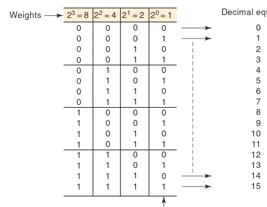
When we deal with binary numbers, we will usually be restricted to a spe-cific number of bits. This restriction is based on the circuitry used to repre-sent these binary numbers. Let’s use four-bit binary numbers to illustrate the method for counting in binary.
The sequence (shown in Figure 1-6) begins with all bits at 0; this is called the zero count.For each successive count, the units (20) position toggles; that is, it changes from one binary value to the other. Each time the units bit changes from a 1 to a 0, the twos (21) position will toggle (change states). Each time the twos position changes from 1 to 0, the fours (22) position will toggle (change states). Likewise, each time the fours position goes from 1 to 0, the eights (23) position toggles. This same process would be continued for the higher-order bit positions if the binary number had more than four bits.
The binary counting sequence has an important characteristic, as shown in Figure 1-6. The units bit (LSB) changes either from 0 to 1 or 1 to 0 with each
count. The second bit (twos position) stays at 0 for two counts, then at 1 for two counts, then at 0 for two counts, and so on. The third bit (fours position) stays at 0 for four counts, then at 1 for four counts, and so on. The fourth bit (eights position) stays at 0 for eight counts, then at 1 for eight counts. If we wanted to
2-3.
= 11.62510
= 8 + 0 + 2 + 1 + 0.5 + 0 + 0.125
+ (1 * 2-1) + (0 * 2-2) + (1 * 2-3) 1011.1012 = (1 * 23) + (0 * 22) + (1 * 21) + (1 * 20)
23 22
1 0 1 1 1 0 1 21 20 2–1 2–2 2–3
Positional values
Binary point
MSB LSB
FIGURE 1-5 Binary position
SECTION1-4/REPRESENTINGBINARYQUANTITIES
13
1. What is the decimal equivalent of 11010112?
2. What is the next binary number following 101112in the counting sequence? 3. What is the largest decimal value that can be represented using 12 bits?
1-4
REPRESENTING BINARY QUANTITIES
In digital systems, the information being processed is usually present in bi-nary form. Bibi-nary quantities can be represented by any device that has only two operating states or possible conditions. For example, a switch has only two states: open or closed. We can arbitrarily let an open switch represent
EXAMPLE 1-2
What is the largest number that can be represented using eight bits?
Solution
This has been a brief introduction of the binary number system and its relation to the decimal system. We will spend much more time on these two systems and several others in the next chapter.
2N-1 = 28-1 = 25510 = 111111112.
count further, we would add more places, and this pattern would continue with 0s and 1s alternating in groups of For example, using a fifth binary place, the fifth bit would alternate sixteen 0s, then sixteen 1s, and so on.
As we saw for the decimal system, it is also true for the binary system that by using Nbits or places, we can go through 2Ncounts. For example, with two bits we can go through counts (002through 112); with four bits we can go through counts (00002through 11112); and so on. The last count will always be all 1s and is equal to in the decimal system. For exam-ple, using four bits, the last count is 11112 = 24-1 = 1510.
2N-1 24 = 16
22 = 4
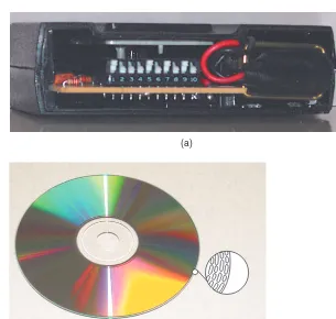
binary 0 and a closed switch represent binary 1. With this assignment we can now represent any binary number. Figure 1-7(a) shows a binary code number for a garage door opener. The small switches are set to form the binary num-ber 1000101010. The door will open only if a matching pattern of bits is set in the receiver and the transmitter.
FIGURE 1-7 (a) Binary
code settings for a garage door opener. (b) Digital audio on a CD.
Another example is shown in Figure 1-7(b), where binary numbers are stored on a CD. The inner surface (under a transparent plastic layer) is coated with a highly reflective aluminum layer. Holes are burned through this reflective coating to form “pits” that do not reflect light the same as the unburned areas. The areas where the pits are burned are considered “1” and the reflective areas are “0.”
There are numerous other devices that have only two operating states or can be operated in two extreme conditions. Among these are: light bulb (bright or dark), diode (conducting or nonconducting), electromagnet (ener-gized or deener(ener-gized), transistor (cut off or saturated), photocell (illumi-nated or dark), thermostat (open or closed), mechanical clutch (engaged or disengaged), and spot on a magnetic disk (magnetized or demagnetized).
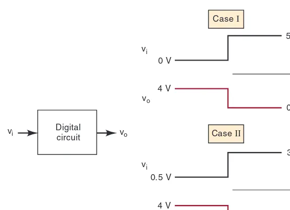
In electronic digital systems, binary information is represented by voltages (or currents) that are present at the inputs and outputs of the various circuits. Typically, the binary 0 and 1 are represented by two nominal voltage levels. For example, zero volts (0 V) might represent binary 0, and ⫹5 V might represent binary 1. In actuality, because of circuit variations, the 0 and 1 would be rep-resented by voltage ranges. This is illustrated in Figure 1-8(a), where any volt-age between 0 and 0.8 V represents a 0 and any voltvolt-age between 2 and 5 V represents a 1. All input and output signals will normally fall within one of these ranges, except during transitions from one level to another.
We can now see another significant difference between digital and ana-log systems. In digital systems, the exact value of a voltage is notimportant;
(a)