Aalto University School of Engineering
Degree Programme in Civil and Structural Engineering
Eero Tommila
Mining method evaluation and dilution control in
Kittilä mine
Master’s Thesis Espoo, May 5, 2014
Supervisor: Prof. Mikael Rinne
Aalto University, P.O. BOX 11000, 00076 AALTO www.aalto.fi Abstract of master's thesis
Author Eero Tommila
Title of thesis Mining method evaluation and dilution control in Kittilä mine Degree programme Structural and building technology
Major/minor European mining course Code of professorship Rak-32 Thesis supervisor Prof. Mikael Rinne
Thesis advisor M.Sc. André van Wageningen
Date 05.05.2014 Number of pages 63 Language English
Abstract
Kittilä mine is a gold mine located in the Northern Finland. It began producing as an open pit mine but nowdays all the production comes from underground mine. The underground mining method was defined during the feasibility study with limited information. With the experience from the underground mining and more rock mechanical and geological data, this thesis was conducted to study if there could be more cost effective method for mining the ore and how to reduce the dilution.
The study is divided into two parts: dilution control and mining method selection. Dilution control was done by identifying the reasons for dilution and examining their impact on Kittilä mine. After this, measures could be developed to decrease dilution and improve predictability. Mining method selection was performed by doing preliminary method selection with traditional mining method selection tools. This yielded several methods, which applicability for Kittilä mine was assessed by terms of safety, suitability, production, dilution & recovery and flexibility. Preliminary selection was followed by stope design, where numerical and empirical methods were used to find stable dimensions for stopes. Stope dimensions, different sequence patterns and level designs were used to create mining scenarios for the deeper, undeveloped parts of the mine. These scenarios were finally compared economically to find the most cost effective solution. Furthermore, three different level heights were compared.
To improve the drilling accuracy it is recommended to survey all the drillhole collars and inclination and redrill the ones that do not meet required criteria. The deviation of the holes can be decreased by using down-the-hole hammer drills instead of top hammer drills. The dilution prediction could be improved by gathering more rock mechanical and geological data. The gathering of this data and utilizing it when designing stope limits could decrease the dilution. The dilution related to overcuts and undercuts can be prevented by systematically bolting these cuts. The proposed mining method is cut-and-fill stoping, which technically is the same as longhole open stoping with delayed backfill that is currently being used. The maximum width of the longitudinal stopes should be increased from 7m to 10m. Stope length and level height should not be changed. The sequence pattern for longitudinal stopes should be primary-secondary-tertiary pattern with 1-4-7 sequencing. Transverse stopes should utilize primary-secondary sequencing.
Keywords Gold, Mining, Mining method selection, Dilution control, Stope optimization
Aalto-yliopisto, PL 11000, 00076 AALTO www.aalto.fi Diplomityön tiivistelmä
Tekijä Eero Tommila
Työn nimi Kittilän kaivoksen louhintamenetelmän tarkastelu ja raakkulaimennuksen kontrollointi
Koulutusohjelma Rakenne- ja rakennustuotantotekniikka
Pää-/sivuaine European mining course Professuurikoodi Rak-32
Työn valvoja Prof. Mikael Rinne
Työn ohjaajaDI André van Wageningen
Päivämäärä 05.05.2014 Sivumäärä 63 Kieli Englanti
Tiivistelmä
Kittilän kaivos on Pohjois-Suomessa sijaitseva kultakaivos. Tuotanto aloitettiin avolouhintana, mutta nykyään koko tuotanto tulee maanalaisesta kaivoksesta. Maanalaisen kaivoksen louhintamentelmä on valittu kannattavuusselvityksessä silloin käytettävissä olleilla tiedoilla. Maanalaisesta louhinnasta saatujen kokemusten, paremman kalliomekaanisen sekä geologisen tiedon perusteella voidaan paremmin tutkia nykyisen louhintamenetelmän mielekkyyttä, sekä miten laimennusta voitaisiin pienentää.
Tutkimus on jaettu kahteen osa-alueeseen: raakkulaimennuksen kontrollointiin sekä louhintamenetelmän valintaan. Raakkulaimennuksen kontrolli on suoritettu tunnistamalla mahdolliset syyt laimennukseen ja tutkimalla niiden vaikutusta Kittilän kaivoksessa. Tämän jälkeen voitiin määritellä keinoja laimennuksen pienentämiseksi ja sen arvioimisen parantamiseksi. Louhintamenetelmän valinta on tehty suorittamalla alustava valinta perinteisillä louhintamenetelmän valintatyökaluilla. Tästä tuloksena saatujen menetelmien käyttökelpoisuutta arvioitiin turvallisuuden, soveltuvuuden, tuotannon tehokkuuden, laimennuksen ja saannin sekä joustavuuden suhteen. Alustavaa valintaa seurasi louhossuunnittelu, jossa louhosten stabiilit dimensiot pyrittiin määrittelemään numeerisilla sekä kokeellisilla menetelmillä. Saatuja dimensioita sekä erilaisia louhintajärjestyksiä käyttäen voitiin tehdä tasosuunnitelmat kaivoksen syväosiin, jonne ei olla vielä edetty. Näiden tasosuunnitelmien pohjalta tehtiin useita louhintaskenaarioita, joiden taloudellisuutta verrattiin. Myös kolmea eri tasoväliä on verrattu keskenään.
Poraustarkkuuden parantamiseksi ehdotetaan että jokaisen porareiän sijainti sekä kaltevuus mitaittaisiin, sekä virheelliset reiät uudelleenporattaisiin. Reikätaipumaa kyetään pienentämään siirtymällä uppovasaraporiin päältä lyövien sijaan. Raakkulaimennuksen arviointia voitaisiin parantaa keräämällä enemmän kalliomekaanista ja geologista dataa, sekä käyttämällä tätä dataa hyväksi louhoksia suunniteltaessa. Ylä- ja alaperiin liittyvää raakkulaimennusta voitaisiin pienentää systemaattisesti vaijeripulttaamalla kyseiset perät. Ehdotettu louhintamentelmä on cut-and-fill stoping, mikä vastaa nykyistä louhintamenetelmää. Pitkittäisten louhosten maksimileveys tulisi nostaa 7m:stä 10m:in. Louhosten pituutta tai tasoväliä ei tulisi muuttaa. Louhosjärjetys pitkittäisille louhoksille tulisi olla kolmen vaiheen louhoksia käyttävä 1-4-7 sekvenssi.
Avainsanat Kulta, Kaivos, Louhintamenetelmän valinta, Raakkulaimennuksen kontrollointi, Louhosoptimointi
Foreword
This thesis was made as a last part of my master’s studies in Aalto University. Studying and writing this thesis has been very interesting and enjoyable, mostly because of the amazing people I have been entitled to work with and to whom I would like to express my gratitude.
The thesis was made possible by Agnico-Eagle and Kittilä mines chief of engineering André van Wageningen. I would like to thank André for presenting me this topic and guiding me all the way from beginning to the very end. My thanks go to all the staff of Kittilä mine, who were helping me with their inputs and making my stay at Kittilä mine enjoyable and memorable. Especially I would like to thank Kyösti Huttu for providing me with necessary information and corrections.
I would like to thank my professors Mikael Rinne, who has been very helpful and supportive not only during this thesis but my whole studies. Mikael also told me about European Mining Course and encouraged me to apply for this program, which resulted in incredible year abroad, lots good friends and massive amounts of information and experience. I would also like to thank other members of staff of the rock engineering department and Aalto University.
I would like to thank all my friends and fellow students for making studying much more fun and pleasant. I could have not done without you.
Lastly I would like to thank my family for supporting me in every possible way, not only during my studies but my whole life. No words can express my gratitude.
Espoo, May 5.2014 Eero Tommila
I
Table of Contents
TABLE OF CONTENTS ... I LIST OF FIGURES ... III NOMENCLATURE ... V LIST OF ABBREVIATIONS ... VI
INTRODUCTION ... 1
Aims and objectives ... 1
Research questions... 1 1 BACKGROUND ... 2 1.1 History ... 2 1.2 Geology ... 2 1.3 Current Operation ... 4 1.3.1 Stope Design ... 5 1.3.2 Level Design ... 5 1.3.3 Sequencing ... 5
2 MINING METHOD SELECTION ... 7
2.1 Hartman Flowchart ... 7
2.2 UBC Method ... 8
2.2.1 Input Values ... 8
2.2.1.1 Geometry of the Deposit ... 8
2.2.1.2 Geotechnical Parameters ... 9
2.2.2 Results ... 9
2.3 Discussion on Mining Methods ... 9
2.3.1 Sub-Level Open Stoping (SLOS) ... 9
2.3.2 Cut-and-Fill Stoping (C&FS) ... 10
2.3.2.1 Transverse Bench Stoping (TBS) ... 10
2.3.2.2 Longitudinal Bench Stoping (LBS) ... 10
2.3.2.3 Avoca ... 11
2.3.3 Vertical Crater Retreat (VCR) ... 12
2.3.4 Square Set Stoping and Stull Stoping ... 13
2.3.5 Drift-and-Fill (D&F) ... 13
2.4 Comparison of Mining methods ... 14
3 STOPE DESIGN ... 15
3.1 Current Design Standards ... 15
3.2 Design Parameters ... 16 3.2.1 In-Situ Stress ... 16 3.2.2 Geotechnical Parameters ... 16 3.2.2.1 RQD ... 16 3.2.2.2 UCS ... 18 3.2.2.3 Joint Sets ... 18 3.3 Numerical Methods ... 20 3.3.1 Input values ... 20 3.3.2 Models ... 21
3.3.3 Results and Evaluation ... 22
3.4 Empirical Methods ... 25
3.4.1 Stability Graph ... 25
3.4.2 Results ... 26
II
4 DILUTION CONTROL ... 28
4.1 Definition of Dilution ... 28
4.2 Effect on Profitability ... 29
4.3 Current Situation ... 30
4.4 Reasons for Dilution ... 30
4.4.1 Drill and Blast ... 30
4.4.2 Planning ... 31 4.4.3 Geotechnical ... 31 4.5 Control Measures ... 35 5 MINE DESIGN ... 37 5.1 Sequencing ... 37 5.1.1 Primary-Secondary Pattern ... 37 5.1.2 Primary-Secondary-Tertiary Pattern (1-4-7) ... 37
5.1.3 Center Out Pattern ... 38
5.2 Level design ... 39
5.2.1 Transverse Bench Stoping ... 39
5.2.2 Longitudinal Bench Stoping ... 40
5.2.3 Avoca ... 41
5.2.4 Theoretical development amounts ... 42
5.2.5 Implementation ... 42 6 FINANCIAL APPRAISAL ... 45 6.1 Input Values ... 45 6.2 Results ... 46 6.3 Sensitivity Analysis ... 47 7 CONCLUSIONS ... 50 8 RECOMMENDATIONS ... 52 REFERENCES ... 53 APPENDIX 1 – MODIFIED STABILITY GRAPH ... I APPENDIX 2 – DILUTION GRAPH BY CLARK ... II APPENDIX 3 – DILUTION GRAPH BY WANG ... III
III
List of Figures
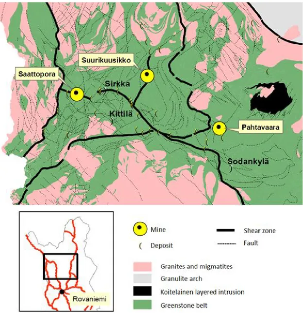
Figure 1.1 Central Lapland greenstone belt and gold deposits in the area (Ojala, 2008). 3
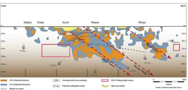
Figure 1.2 Longitudinal section of the deposit (Agnico-Eagle, 2013) ... 4
Figure 1.3 Cross section of the deposit, displaying rock types (Agnico-Eagle, 2013) .... 4
Figure 1.4 Example of level design in Kittilä mine (Agnico-Eagle, 2013) ... 5
Figure 1.5 Stoping sequence (Agnico-Eagle, 2013) ... 6
Figure 2.1 Hartman flowchart (Hartman, 1987) ... 7
Figure 2.2 Thickness of the ore defined by stope widths ... 8
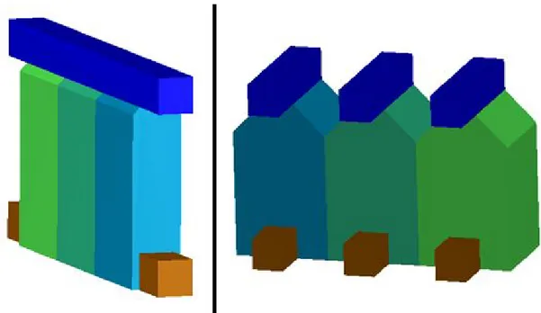
Figure 2.3 Sketch of LBS and TBS, showing undercuts, overcuts and three stopes ... 11
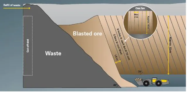
Figure 2.4 Avoca method (Villaescusa & Kugantahan, 1998) ... 11
Figure 2.5 Tight fill Avoca (Atlas Copco, 2007) ... 12
Figure 2.6 VCR (Atlas Copco, 2007) ... 13
Figure 3.1 Distribution of RQD-values in ore zone, FW and HW, derived from drill cores ... 17
Figure 3.2 Comparison of RQD-values distribution in the ore zone in top parts of Suuri and Roura ... 18
Figure 3.3Contour plot of joints with two main joint directions showing dip/dip direction (Syrjänen, 2007) ... 19
Figure 3.4 Contour plot of joints (Storvall & Lindfors, 2013) ... 20
Figure 3.5 Correlation between RQD and GSI, based on geotechnical logging of six boreholes ... 21
Figure 3.6 Profiles used in analysis ... 22
Figure 3.7 Different profile widths, colored by σ1 ... 23
Figure 3.8 Different stope lengths, colored by σ1 ... 23
Figure 3.9 Stresses of 25m high transverse stope, colored by σ1 ... 24
Figure 3.10 Relaxation zones around 25m high, 15m long and 10m wide stope ... 24
Figure 3.11 Supporting diagrams for stability graph (Clark & Pakalnis, 1997) ... 26
Figure 4.1 Planned and unplanned dilution (Mitri, et al., 2010) ... 28
Figure 4.2 Definition of ELOS (Clark & Pakalnis, 1997) ... 29
Figure 4.3 Graph showing relation of dilution and revenue ... 30
Figure 4.4 Possible effects of poor drilling accuracy ... 31
Figure 4.5 Stope height effect on ELOS, based on mined stopes ... 32
Figure 4.6 Stope width effect on ELOS, based on mined stopes ... 33
Figure 4.7 Example of cavity scan of transverse stope limit in brown and cavity scan in yellow (Agnico-Eagle, 2013) ... 33
Figure 4.8 Crosscut of stope looking north showing typical origins of dilution in transverse stope shown in red ... 34
Figure 4.9 Comparison of ELOS and RQD of mined stopes ... 34
Figure 4.10 Distribution of failed stopes in different stope categories ... 35
Figure 4.11 Crosscut of stope looking north showing cablebolt design for over- and undercuts of transverse stope, cablebolts shown in blue ... 36
Figure 5.1 Primary-secondary pattern (Ghasemi, 2012) ... 37
Figure 5.2 1-4-7 pattern (Ghasemi, 2012) ... 38
Figure 5.3 Center out pattern (Ghasemi, 2012) ... 39
Figure 5.4 Level design for TBS ... 40
Figure 5.5 Level design for LBS, primary-secondary pattern ... 40
Figure 5.6 Level design for LBS, 1-4-7 pattern ... 41
IV
Figure 5.8 Amount of OPEX development in different scenarios ... 43
Figure 5.9 Ratio of paste- and rockfill in different scenarios ... 43
Figure 5.10 Ratio of transverse and longitudinal stopes in different scenarios ... 44
Figure 6.1 Comparison of production costs per gold ounce in different scenarios and level heights ... 46
Figure 6.2 Sensitivity plot ... 47
Figure 6.3 Effect of dilution on production costs for different level heights ... 48
Figure 6.4 Effect of waste grade on production costs for different level heights... 48
Figure 6.5 Effect of development meters on production costs for different level heights ... 49
V
Nomenclature
σH Major horizontal stress (in-situ) σh Minor horizontal stress (in-situ) σv Vertical stress (in-situ)
σ1 Major stress resultant (induced) σ3 Minor stress resultant (induced)
kv Ratio of horizontal stress and vertical stress (σH/ σv) kh Ratio of horizontal stresses (σH/ σh)
E Modulus of elasticity v Poisson’s ratio N’ Stability number
Q’ Tunneling quality index mi Petrographic constant D Disturbance factor
VI
List of Abbreviations
AB Aktiebolaget – Limited Company CLGB Central Lapland Greenstone Belt D&F Drift-and-Fill
DC Diamond Core (Drilling) DTH Down-the-hole
ELOS Equivalent Linear Overbreak Sloughing ELRD Equivalent Linear Relaxation Depth
FW Footwall
GSI Geological Strength Index
GTK Geologian Tutkimuskeskus – Geological Survey of Finland
HW Hanging Wall
LBS Longitudinal Bench Stoping Ltd. Limited Company
Oy Osakeyhtiö – Limited Company RMR Rock Mass Rating
RQD Rock Quality Designation SLOS Sub-Level Open Stoping TBS Transverse Bench Stoping UBC University of British Columbia UCS Uniaxial Compression Strength VCR Vertical Crater Retreat
1
Introduction
Kittilä mine is a gold mine located in Northern Finland. It started producing in 2009 as an open pit and gradually moved to underground mining. In 2013 all production came from the underground mine. The underground mining method and design parameters were defined during the feasibility study of the mine. The primary mining method is longhole open stoping with delayed backfill utilizing transverse stopes. Longitudinal stopes are used when mining narrow ores. Transverse stoping requires high amount of development leading to high production costs, while longitudinal stoping has been causing heavy dilution.
As there is now experience from underground mining and more rock mechanical and geological data is available, it was decided to conduct a study to review the current mining method and to examine how excessive dilution could be prevented. This thesis is focused on improving the dilution control and finding the optimal mining method and design parameters for the Kittilä mine.
Aims and objectives
The goal of this thesis can be expressed by the two following objectives:
• Determine measures to reduce dilution.
• Determine the most suitable mining method for Kittilä mine.
Research questions
As these objectives are still very broad and general, several research questions will be developed in order to narrow down the focus of the study. These research questions also help in reaching the objectives and defining the structure of the thesis.
Objective: determine measures to reduce dilution.
• What are the factors that can influence dilution?
• What is their impact in Kittilä mine?
• What can be done to prevent dilution?
Objective: determine the most suitable mining method for Kittilä mine.
• What are the possible mining methods for this kind of ore and geological setting?
• What is their suitability for Kittilä mine?
2
1
Background
1.1
History
The first signs about mineralization in the area were received in 1986, during regional gold exploration by GTK. At the same time the road from Kittilä to Pokka was under construction and the outcrops revealed by road cuttings were examined by geologists. Near Vuomajärvi, about four kilometers from the current deposit, geologists Jorma Valkama and Pekka Puhakka saw visible gold in one of these outcrops. This particular gold pocket revealed to be quite small, but it showed that the area has potential for gold. GTK continued to investigate the area with low-altitude airborne magnetic and electromagnetic surveying. Based on this information DC drillings were made in the Suurikuusikko and Rouravaara area. The drillings proved that there was gold in the area in relatively good grades. However, the gold turned out to occur mostly as refractory gold, thus requiring more sophisticated processing than free gold. (Pankka, et al., 2006) In 1998 the rights for the claim were sold to Swedish exploration company Riddarhyttan Resources AB, which continued the drillings, mapping the resource and also test mining. As the exploration continued the resources expanded and a mine seemed to look possible. Riddarhyttan received mining permit in 2003. In 2005 Riddarhyttan was acquired by Canadian company Agnico-Eagle Mines Ltd. The decision to construct the mine came in 2006 and production from open pit began in 2008. (Riddarhyttan Resources AB, 2003) (Agnico-Eagle, 2013)
1.2
Geology
The deposit is located within the central Lapland greenstone belt (CLGB), a belt of Paleoproterozoic, volcanic and sedimentary rocks lying on top of the Archean basement. The CLBG was formed roughly 2 billion years ago due to volcanic activity in the area and has gone through several geological processes after that, like rifting and faulting. The greenstone belts all over the world are known for their potential to host gold deposits and CLBG is no different as can be seen from the Figure 1.1. CLGB is still fairly unexplored in terms of mineral deposits, so there are still lots of possibilities in the area. (Ojala, 2007)
3
Figure 1.1 Central Lapland greenstone belt and gold deposits in the area (Ojala, 2008)
The Suurikuusikko deposit is located in the Kiistala shear zone. This shear zone is over 25 kilometers long and holds several individual gold bearing lodes along its length. The largest concentration of these lodes occurs in the Suurikuusikko area. The gold is mineralized in the shear zone by hydrothermal process. The strike of the mineralizations varies from north to north-east, plunges to north and is dipping almost vertical (Figure 1.2 and Figure 1.3). The gold occurs mostly as refractory within arsenopyrite (75%) and pyrite (21%), rest is found as free gold (4%). (Agnico-Eagle, 2013)
4
Figure 1.2 Longitudinal section of the deposit (Agnico-Eagle, 2013)
Figure 1.3 Cross section of the deposit, displaying rock types (Agnico-Eagle, 2013)
1.3
Current Operation
The production began as open pit operation. The ore was mined consecutively from two open pits, Suuri and Roura. The pits began to approach their design depth and production moved gradually to underground mining. In 2012 the last blasts from the open pits were made and in 2013 all production came from the underground mine. The underground mine is currently being accessed from one portal. From the decline the two operating parts, Suuri and Roura, are accessed with two ramps and series of footwall drifts. The production areas are still relatively shallow (<500m) so all the ore is hauled by fleet of trucks by the decline. The production is currently 1,1 Mt/a, but an expansion of the processing plant is ongoing and will increase the annual processing capacity to 1,5 Mt.
5
1.3.1 Stope Design
The stopes are designed as 15m long along the strike of the ore and the width is determined by thickness of the ore. The basic design height is 25m, however, in top parts of the Roura 40m high stopes are being used. The stopes have two accesses: overcut and undercut. Overcut is used for drilling, charging and backfilling while undercut is used for mucking. All the stopes are backfilled, primary stopes with paste fill or cemented rockfill and the secondary stopes with rockfill.
1.3.2 Level Design
The mining method currently used in Kittilä mine is longhole open stoping with delayed backfill. This method will be referred as cut-and-fill stoping in this thesis. The ore is accessed via footwall drifts that are developed in the waste, parallel to the strike of the ore. The distance between the footwall drift and the ore is set to be at least 20 meters. From these footwall drifts, overcuts and undercuts are driven into the ore, perpendicular to strike. This is called transverse bench stoping (TBS). However, when the ore gets thinner than 7m the stopes are done parallel to strike, leading to longitudinal bench stoping (LBS). A typical level design can be seen in the Figure 1.4. In the figure the drifts are displayed in blue, transverse stopes in purple and longitudinal stopes in cyan. The figure also illustrates well the amount of development needed when mining transverse stopes.
Figure 1.4 Example of level design in Kittilä mine (Agnico-Eagle, 2013)
1.3.3 Sequencing
The basis of the stope sequencing is bottom up primary-secondary sequencing. Mining starts from the middle of the sill level and gradually expands both horizontally and vertically. This sequencing is shown in the Figure 1.5 Stoping sequence. The yellow stopes are primary and blue ones are secondary. The secondary stopes can be mined only after all the primary stopes around them are mined and backfilled. Actual sequence is affected by the grades and sizes of the stopes and the sequence pattern is not strictly followed.
6
Figure 1.5 Stoping sequence (Agnico-Eagle, 2013)
The longitudinal stopes are mined using retreat sequencing. This means that mining starts from one end of the ore and progresses stope by stope along the strike to the other end. In this kind of sequence every stope needs to be backfilled with consolidated fill.
7
2
Mining Method Selection
Selection of mining method is very important, since it is one of the most influential factors in the success of the mine. Even though several methods are technically available, they may result in much different economic performance. This is the reason the selection should be done carefully and not just the pick one that seems practical. During the history several tools for method selection have been developed. However, they mostly rely on geometry and geotechnical properties of the deposit and these methods should only be used as preliminary investigations in the selection procedure. The final decision about the mining method to be used should be based on financial analysis of the methods that are chosen in the preliminary phase.
In this thesis the preliminary mining method selection will be done by using flow chart designed by Hartman (Hartman, 1987) and the UBC method (Miller-Tait, et al., 1995). After this their applicability for the Kittilä mine will be discussed, ruling out the unsuitable methods by comparing their safety, suitability, production rate, dilution, recovery and flexibility.
2.1
Hartman Flowchart
Hartman developed a flowchart for defining the mining method. This chart is qualitative and it is mainly based on the geometry of the deposit, with some reference to the ground conditions. This method should only be used as an approach to the proper method selection. Chart (Figure 2.1) is very quick and easy to use. As the open pit has already been mined so only deep deposit options are being investigated. Then, applying the geometrical properties of the deposit: tabular, steep and thin and moderate strength yields the result of shrinkage stoping, cut-and-fill stoping and stull stoping. (Hartman, 1987)
8
2.2
UBC Method
The UBC method (Miller-Tait, et al., 1995) is based on Nicholas method (Nicholas, 1981), difference being the use of RMR for ground conditions instead of RQD used in Nicholas method and the depth of the deposit in the geometry section. UBC is quantitative method, meaning it gives different methods points and then ranks them according how many points they received. The points come from two categories: the deposit geometry and the ground conditions, which are further divided into the strength of hanging wall (HW), ore and footwall (FW). The points given go from one to five and if the condition outrules a method, it receives -49 points. (Darling, 2011)
2.2.1 Input Values
2.2.1.1 Geometry of the Deposit
The geometry of the deposit is being defined by five factors. First, is the general shape, which can be massive, tabular or irregular. As the ore in Kittilä is in lenses, platy-tabular is one to choose. Second is the thickness of the ore, this is a bit more complicated since lenses close to each other can be considered as one making the ore much thicker.
The thickness is defined by looking at the distribution of stope widths seen in Figure 2.2. Stopes are defined as 15m long sections along the strike of the ore. If the grade inside the ore lens of such 15m section is above cutoff grade it is defined as mineable stope. As 75% of the stopes are less than 10m wide, the ore is classified as narrow (3-10m). Third factor is the plunge, as the ore dips almost vertically it is definitely steep. Fourth represent the grade distribution. The gold grade can change very quickly over relatively short distances so it can be considered as erratic. Last variable is the depth of the deposit. The stopes have depths varying from 75m to 1175m so one single option does not cover this, therefore two separate calculations need to be done for intermediate (100m-600m) and deep (more than 600m).
Figure 2.2 Thickness of the ore defined by stope widths 5 % 47 % 23 % 14 % 11 %
Ore Thickness
<5m 5m-7,5m 7,5m-10m 10m-15m >15m9
2.2.1.2 Geotechnical Parameters
The geotechnical information is divided into two parts: the RMR and the UCS of the Ore. Both of these are applied to ore zone, HW and FW.
There currently is no available data about the RMR in the mine, but RQD values are logged from the DC drilling. RQD is only one factor when calculating RMR, but since no better data is available, RQD will be used to estimate the rock mass conditions. The mean RQD values from the stopes mined so far and stopes to be mined in near future are 52 for the ore, 47 for FW and 56 for HW. These will be classified as weak for HW and medium for ore and HW.
The rock substance strength is defined by ratio of UCS and main principal stress. As the stress is dependent on the depth, separate analysis needs to be done for the deeper and shallower parts. The estimated major horizontal stresses are 40MPa for the deep part and 20MPa for the shallower part (Ask, 2013). The UCSs are obtained from the laboratory tests (Eloranta, 2012). These values result in weak rock substance strength in all the zones in shallow case and very weak for deep.
2.2.2 Results
Parameters obtained were applied to a tool developed by EduMine (EduMine, n.d.), the results can be seen in Table 2.1.
Intermediate (100-600m) Deep (>600m)
Cut-and-Fill Stoping (37) Cut-and-Fill Stoping (33) Sublevel Stoping (27) Square Set Stoping (25)
Open Pit (26) Sublevel Stoping (21) Shrinkage Stoping (26) Shrinkage Stoping (21) Square Set Stoping (20) Top Slicing (16)
Top Slicing (14) Block Caving (-18) Sublevel Caving (-21) Longwall Mining (-19)
Block Caving (-22) Open Pit (-22) Longwall Mining (-22) Sublevel Caving (-22)
Room and Pillar (-33) Room and Pillar (-34) Table 2.1 Results of UBC method (EduMine, n.d.)
2.3
Discussion on Mining Methods
2.3.1 Sub-Level Open Stoping (SLOS)
SLOS received good ranking in the UBC method being the 2nd and 3rd option for intermediate depth and deep part. However, the Hartman flowchart does not consider SLOS as option for narrow ore. SLOS is quite common method used in underground mining, due to high production and being easily mechanized. Drilling is done in rings from sublevels allowing usage of large mass blasts and mucking is done at the bottom of the stopes. As the name implies, stopes are left open after they are mined out. Naturally, this causes stability problems, which is why pillars need to be left between the stopes. This leads to low initial recovery, which is not desired, since the ore in Kittilä mine is highly valuable. Also, the large open stopes are prone to high dilution especially in weak rock. The flexibility of this method is low since mining usually
10
progresses gradually from one end of the orebody to the other. Using remote controlled LHDs allows the stopes to be non-entry zones, so SLOS can be considered a safe method.
2.3.2 Cut-and-Fill Stoping (C&FS)
Cut-and-fill stoping proved to be best method according the UBC method and the Hartman flowchart also identified it as viable method. C&FS is basically the same method that is currently in use at Kittilä mine. The drilling is done from overcuts and mucking from undercuts. In terms of mechanization and safety this method is very similar to SLOS. However, when all the stopes are backfilled there is no need for pillars and thus initial recovery is high. Stoping operations use mass blast which leads to moderate dilution at best, depending on the stope size. C&FS is very flexible and is suitable to orebodies of almost all shapes. There are mainly two variations for C&FS, transverse bench stoping and longitudinal bench stoping.
2.3.2.1 Transverse Bench Stoping (TBS)
In TBS the production drifts are driven perpendicular to the strike of the ore. The stopes are opened by doing a slot raise, usually near the back end of the stope and the production then proceeds by ring blasting.
The TBS is a widely used method due to having several advantages. The planning is easy since all the stopes can have very similar dimensions, thus simplifying the design. The other important thing about planning is that TBS is highly flexible sequencing wise, meaning that there are lots of possibilities in which order the stopes can be mined. The similarity of the stopes also makes mechanization easier due to repetitive processes, leading to high tonnages.
The most serious disadvantage of the TBS is the fact that every stope needs its own draw points, thus requiring lots of development. This problem gets more severe when mining narrow veins since the amount of supporting development stays the same while stopes get smaller. The other set back with narrow ore is that all the stopes requires the slot raise, as the stopes get smaller this starts to increase the drill meters per ton of ore and cycle times of stopes.
2.3.2.2 Longitudinal Bench Stoping (LBS)
LBS is very similar to TBS but the production drifts are driven parallel to the strike of the ore. This means that more of the production drifts are driven in the ore itself, thus reducing the development in the waste. The production of the stope is done similarly as in TBS, doing a slot raise and then blasting rings.
The LBS suits well for narrow veins, since the lenths of the stopes are not limited by the thickness of the ore. This means possibly fewer slot raises, and less development in the waste per ton of ore than in TBS, depending on the maximum stable stope length.
Planning in LBS is bit harder since the geometry of the stopes is more dependent on the ore geometry, making the blast ring design more complicated. LBS is also less flexible since stopes are accessed from adjacent stopes.
11
Figure 2.3 Sketch of LBS and TBS, showing undercuts, overcuts and three stopes
2.3.2.3 Avoca
The Avoca mining method can be described as longitudinal retreat mining or LBS with continuous backfill. The production is the same as in LBS, the difference is with the backfilling. In LBS the stopes are mucked empty and then backfilled. Avoca introduces backfilling at the same time as mining proceeds. The idea behind this is that there would basically be no limit for stope length. As the stopes can be larger there will be less slot raises to be made, thus making production faster and less drilling and faster cycle times. In Avoca the stopes need to be accessed from both sides, the front end of the stope is used for mucking, drilling and charging, while the back end is used for backfilling. This introduces limitations to sequence as the mining progresses linearly from one end to another. The other problem with Avoca is the huge amount of waste rock needed for backfilling. If there is not enough waste from the underground development, a shaft would be needed to bring waste from the surface.
12
One modification for Avoca, named tight fill Avoca, is to keep the stopes almost fully filled. As a result, the ore will be blasted against the backfill, called buffer blasting or choke blasting. Blasting against the backfill causes extra dilution or possibly ore losses as the ore and rockfill gets mixed. The dilution and recovery can be controlled by systematically using cavity monitor scanning. However, this causes lot of work and requires good coordination between planning and production. The advantage of keeping the stope filled is that the open surface of the HW and FW is smaller, leading to less sloughing and therefore less dilution from HW and FW.
Figure 2.5 Tight fill Avoca (Atlas Copco, 2007)
2.3.3 Vertical Crater Retreat (VCR)
Shrinkage stoping was placed 4th in the UBC method and was also included in the Hartman flowchart. VCR is a modernized version of shrinkage stoping. The main difference between the two is that in VCR drilling and charging is done from the overcut making it much safer than shrinkage stoping, where this is done from inside the unsupported stope. This also makes mechanization easier, thus making VCR more productive.
In typical stoping ore is blasted in rings, extracting vertical slices from the orebody. In VCR this is done by blasting craters to the bottom part of the ore, extracting horizontal slices. The main benefit from this is that no slot raises are required since the void for expansion is below the ore, undercut in the first blast and the open stope area in the subsequent blasts. This lack of slot raises reduces the amount drillmeters needed for the stope. Other benefit is that the blasts will be done as soon as there is enough void for one slice to expand. The stope is emptied only after all the ore is blasted thus keeping the time stope is open at minimum, increasing the stability.
The downside of the VCR is the complexity of blasting. Since the same drillholes are used for every blast, it is vital for optimal performance to know exactly where to place charges and holes need to stemmed below and above the charge. The spherical charges used in cratering technique usually have the length of six times the hole diameter, so the height of the extracted slice is directly proportional to the hole diameter. This is why the diameters used in VCR are usually 140mm or 165mm.
13
The mine design of VCR is very similar to TBS, therefore they have mostly the same strengths and weaknesses. The main difference is that VCR is not very well suited for narrow ore due to utilization of large diameters for drilling.
Figure 2.6 VCR (Atlas Copco, 2007)
2.3.4 Square Set Stoping and Stull Stoping
Square Set Stoping proved to be the 2nd best option for the deep parts in the UBC method, while Stull stoping appeared in the Hartman flowchart. Both of these methods are artificially supported methods, usually with timber. Both are very labor intensive and have low degree of mechanization, resulting in low production rates. The advantages of these methods are that they can follow the orebody closely allowing high selectivity and low dilution. Building timbered support requires workers to enter the unsupported stopes making them unsafe methods.
2.3.5 Drift-and-Fill (D&F)
D&F is not mentioned in neither of the used mining method selection tools, but it is one possible method for this type of ore. D&F is a mining method that was frequently used before the longhole drills came popular. This method is suitable for steeply dipping narrow veins hosting high grade ore. The production is done from drifts driven into the ore rather than stopes. This minimizes the development in the waste since there is no need for the footwall drifts. Although, the ore in Kittilä mine is very disseminated
14
which would require extracting lot more waste. As all the ore comes from drifting the blast are small, which enables low dilution and high selectivity. However, the production is lower due to less ore from single blast, usually leading to higher cost per ton than with stoping methods. The flexibility of D&F is not very good, since there are only few production areas.
2.4
Comparison of Mining methods
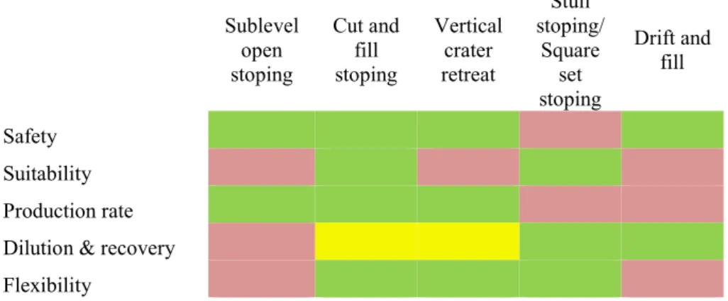
The comparison of mining methods was done in terms of safety, suitability, production rate, dilution & recovery and flexibility. The method was considered unsafe if the workers have to work in areas of unsupported rock. Suitability means if the method can be effectively applied to this kind of ore. Production rate is defined by how labour intensive the method is. Dilution refers to planned and unplanned dilution that will end up in the mill feed while recovery means how much of the ore cannot be mined or mucked, including possible pillars. Methods are given colors to measure their applicability: green for applicable, red for not applicable and yellow for neutral. For further elaboration see 2.3 Discussion on Mining Methods.
Sublevel open stoping Cut and fill stoping Vertical crater retreat Stull stoping/ Square set stoping Drift and fill Safety Suitability Production rate Dilution & recovery Flexibility
Table 2.2 Comparison of mining methods
Table 2.2 presents the comparison of the mining methods. From this table it can be concluded that Cut-and-fill stoping would be the most suitable mining method for Kittilä mine. From this point onwards, all the design is done based on this method.
15
3
Stope Design
Stope design is an important part in the mine planning since its influence on overall success is quite influential. The basic idea is to create as large stopes as possible to minimize the cost per ton. However, if the stopes are too large the problems with stability can cause excess dilution, ore losses and delays, thus retarding profitability.
3.1
Current Design Standards
The current design for stopes is based on three studies made about the dimensions of the stopes. These are the original underground geotechnical study by Piteau Associates (Rose, 2000), Kittilä underground mine stability analysis by WSP Gridpoint (Syrjänen, 2007) and the rock mechanics study of Kittilä mine deep expansion by KMS Hakala Oy (Hakala, 2009).
In the Piteau study it was concluded that stopes of 25m high and 30m wide should be possible. However, even in the report itself it was noted that the parameters used in this study do not have the sufficient accuracy to provide reliable information and that further investigations should be done. This study was based on stability graph method, which will be explained in more detail in part 3.4 Empirical Methods. (Rose, 2000)
The second study was performed by WSP Gridpoint in 2007. This study also relied on the stability graph method, with stress analysis made with Examine 3D program. The background information was obtained from geological block model, made by Gridpoint Finland Oy. This study was investigating stopes 15m long, 12m wide and the heights of 25m, 35m and 45m. The recommendation from this report was to use 25m high stopes below level 400. Above this level, 35m and even 45m high stopes may be possible. (Syrjänen, 2007)
The third study was made by KMS Hakala Oy in 2009 to ensure stope stability when proceeding deeper. Stability graph method was used, together with Examine 3D program for stress calculations. The input parameters were obtained from drillhole data. The stope dimensions used were 15m wide, 15m long and heights of 25m and 50m for transverse stopes and 7m wide, 25m high and lengths of 25m and 50m for longitudinal stopes. The recommendations were not to increase the stope dimensions. However, increasing dimensions might be possible in good rock, but further investigations are needed. (Hakala, 2009)
Based on these studies it was decided to use 25m sub-level height except for the top parts of Roura where 40m is the height. The transverse stopes are designed to be 15m in lentgh and maximum width of 35m. Longitudinal stopes have been tested with lengths up to 60m with varying success. The optimum length is not yet determined.
All of the studies implied that the rock mechanical data available was not sufficient to perform reliable calculations. Especially the lack of stress measurements was seen as a major setback.
16
3.2
Design Parameters
3.2.1 In-Situ Stress
The lack of stress measurements has a high influence on creditability of rock mechanical calculations. To overcome this problem, a study was made in 2013 in order to get better idea about the stress field. The study was performed by Pöyry SwedPower AB (Ask, 2013) and was done by hydraulic breaking method. The results can be seen in Table 3.1. Depth 375m 650m σv (MPa) 9,0-9,7 18 σh (MPa) 9,3-10,3 13,9 σH (MPa) 12,1-24,2 26,6 σH trend 79-83° 75°
Table 3.1 Results of stress measurements (Ask, 2013)
During the testing there were difficulties due to stability problems, high water pressure and high fracture frequency. This limited the amount of data, thus reducing the reliability of these results. The assumptions for calculations can be seen below, where kv is the ratio of vertical stress and major horizontal stress and kh is the ratio of horizontal stresses.
• Gradient for σv is 0,029MPa/m • Direction of σH is 75°
• Dip of horizontal stresses is 0º.
• kv value is 1,5 • kh ratio is 2
Vertical stress is directly proportional to the weight of the rock above so the gradient is derived from density of 2,9t/m3. The direction of the major horizontal stress, k
h ratio and the kv value are from the measurements in the depth of 650m as this was considered more reliable than the measurements in the depth of 375m.
3.2.2 Geotechnical Parameters
In order to calculate stope stabilities, certain parameters are required. Acquiring the information is an important part in the design, since wrong base values will lead to inaccurate results, rendering them unreliable if not useless. So far, very little mapping has been done at the mine so most of the needed rock mechanical data will be acquired from the drill cores and block model.
3.2.2.1 RQD
RQD is basically an indicator of fracture spacing and is currently the only available information about the rock mass condition that has sufficient coverage. It has strong influence on both Q’ and GSI, rock mass rating systems that will be used in the calculations later on.
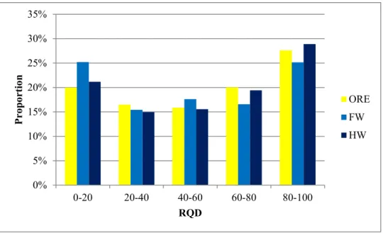
The RQD values for ore zone, FW and HW are derived from the block model or drill cores. Ore zone is defined by all the stopes that are on the current life of mine and FW and HW are 5m wide zones in both sides of these stopes. The distribution of these values can be seen in the Figure 3.1.
17
Figure 3.1 Distribution of RQD-values in ore zone, FW and HW, derived from drill cores
From the figure it can be seen that the distribution of RQDs is quite similar, FW being bit worse than HW and ore zone. At the Table 3.2 average RQD-values for different areas are presented, as well as portion of weak rock in these areas. Rock is defined weak when its RQD-value is less than 40.
Average RQD/Percentage of weak rock
Suuri Roura Rimpi
Top 56/25% 55/32% 51/30% Deep 69/8% 62/17% 80/1%
Table 3.2 RQD-values in different areas, derived from block model
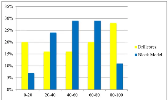
The average values are moderate in top parts and good in the deep parts. The amount of weak rock also indicates that the rock mass quality is better in the deep areas. These values are acquired from the block model, which may cause that they are biased towards the mean values, since smaller sections of good and poor rock are being evened out within the blocks. This can be seen in the Figure 3.2, where the RQD-values obtained from drill cores and block model are being compared. This figure indicates that the portions of weak rock shown in Table 3.2 are probably lower than in reality. The difference between average RQDs from drill cores and block model was insignificant.
0% 5% 10% 15% 20% 25% 30% 35% 0-20 20-40 40-60 60-80 80-100 Pr op or tion RQD ORE FW HW
18
Figure 3.2 Comparison of RQD-values distribution in the ore zone in top parts of Suuri and Roura All the values are derived from the drillcores. This may cause slight error, since the RQD logging is done from the drillcores used for exploration purposes rather than geotechnical cores. This kind of coring may cause some additional breaking, thus increasing the portion of low RQDs.
3.2.2.2 UCS
Series of laboratory tests were conducted in Aalto University to find UCS, E and v for the most common rock types of Kittilä mine. The ore zone, HW and FW consist mostly of mafic metaigneous rocks (MML, MVX and MDY), these make up about 80%. The last 20% consists of felsic metaigneous (FIN), metavolcanogenic sedimentary (AVS) and metasedimentary (CHT) rocks. In the weak rock graphitic zones (GFZ) are also present, occurring mostly in sections of about 20cm, but even zones of several meters exists. GFZ is clearly the weakest rock with UCS of only 14,1 MPa and E of 1,4 GPa. (Eloranta, 2012) (Agnico-Eagle, 2013)
For the modeling purpose, values for weak and moderate rock mass were estimated using data from the drillcores from top parts of Suuri and Roura. As a result, following values will be used:
• Moderate rock mass o UCS = 132 MPa o E = 69 GPa o v = 0,25
• Weak rock mass o UCS = 89 MPa o E = 61 GPa o v = 0,24
3.2.2.3 Joint Sets
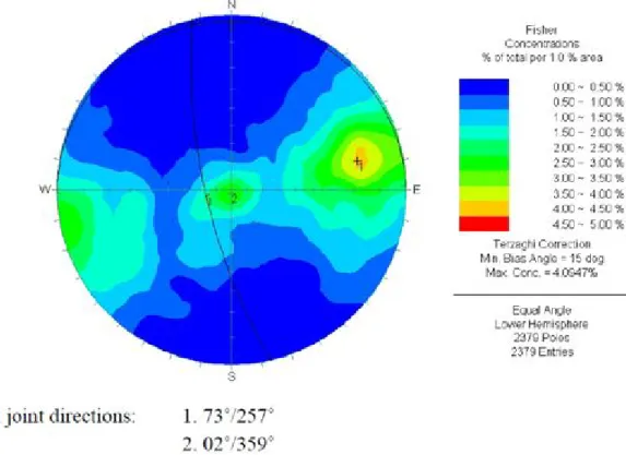
From logging of six geotechnical boreholes it was noted that in most cases there were two joint sets plus random. The categories three plus random and four or more joint sets consisted 31% of all the samples. Near the ore zones the rock mass seems to get more jointed, which would be logical since the ore is located in the shear zone. This data is
0% 5% 10% 15% 20% 25% 30% 35% 0-20 20-40 40-60 60-80 80-100 Drillcores Block Model
19
based on six boreholes, of which only four intersects the ore zone, therefore it is not very reliable. The joint orientations can be seen in two contour plots in Figure 3.3 produced by WSP (Syrjänen, 2007) and Figure 3.4 by Itasca consultants (Storvall & Lindfors, 2013). The plots show only low concentrations of joints but indicate that the joints with east or west dip direction are more common. Plot made by Syrjänen also shows increased density of vertical and almost vertical joints. Plot made by Itasca shows no concentration of vertical joints, which may be result of plotting of only one hole, which was also vertical. These concentrations seem logical, since they are parallel to the shear zone in which the ore body lies.
Figure 3.3Contour plot of joints with two main joint directions showing dip/dip direction (Syrjänen, 2007)
20
Figure 3.4 Contour plot of joints (Storvall & Lindfors, 2013)
3.3
Numerical Methods
Numerical modeling of the stopes is performed using program Examine 3D by rocscience. This program uses boundary element method to study three dimensional excavations. The main reason for building numerical models is the stress analysis. The goal is to provide information about induced stresses for the stability graph method and to determine the relaxation zones around the stopes.
3.3.1 Input values
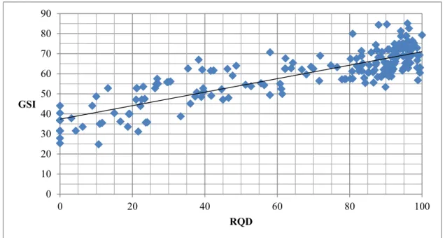
The calculations were made for two different rock types: weak and moderate. Failure criterion that is used is Hoek-Brown (Hoek, et al., 2002). This criterion utilizes intact rock strength parameters and scales them with GSI, petrografic constant mi and disturbance factor D. These factors are easier to obtain than friction angle and cohesion used in Mohr-Coulomb failure criterion, which is why Hoek-Brown is used. Strength parameters for intact rock were given in the section 3.2.2.2. GSI values are estimated from the RQD values. In Figure 3.5 are RQD and GSI values from six boreholes, where geotechnical logging has been made. From the graph a correlation between the two can be made and is expressed as follows:
𝐺𝑆𝐼= 0,33∗ 𝑅𝑄𝐷+ 37
The average RQD-value for weak rock is 14,2 and for moderate 49,8. Using the formula above these would render to GSI values of 42 and 53. The mi is determined to be 17, a value typical for similar rocks found in the Kittilä mine. Disturbance factor is set to 0,7 due to production blasting of the stopes.
21
Figure 3.5 Correlation between RQD and GSI, based on geotechnical logging of six boreholes The constants for calculating stresses were defined in section 3.2.1. As these derived constants are not very reliable, several different values for kv and kh are studied in order to investigate the effect of stress. The direction of major horizontal stress is perpendicular to the strike of the longitudinal stopes and parallel to transverse ones in all cases. Calculations will be performed to stopes at depth of 1000m, following values will be used:
Case 1 2 3
σv 30 MPa 30 MPa 30 MPa σH 44 MPa 60 MPa 60 MPa σh 22 MPa 22 MPa 30 Mpa
Table 3.3 Stress resultants for numerical models
3.3.2 Models
In the analysis total of 9 different profiles were used. These are divided between three different level heights: 30m, 25m and 20m and three different profile widths: 5m, 10m and 15m. All the profiles used can be seen in the Figure 3.6. All the profiles were further analyzed in three different lengths: 15m, 30m and 60m. The orientation of the stopes was mostly done so that the strike of the stope is perpendicular to the major principal stress, this means longitudinal stopes. For transverse stopes, 15m wide and 15m long with heights of 20m, 25m and 30m are used.
0 10 20 30 40 50 60 70 80 90 0 20 40 60 80 100 GSI RQD
22
Figure 3.6 Profiles used in analysis
3.3.3 Results and Evaluation
Rock quality had no visible effect on the stress distribution around stopes. This leaves four different variables: profile width, length of the stope, height and stress combination. Figure 3.7 and Figure 3.8 show comparison of different profile widths and different stope lengths. There are several things to be noticed in these figures. First, the side walls (HW and FW) become relaxed, meaning that σ3 is less than zero. Second, highest stresses are induced in the roof and become even greater when length is increased. Third, profile width has little effect on stresses on roof or side walls. Fourth, the stresses in the end walls are affected only by profile width, the narrowest profile inducing higher stresses than the rest.
23
Figure 3.7 Different profile widths, colored by σ1
Figure 3.8 Different stope lengths, colored by σ1
In Figure 3.9 the stresses of a transverse stope can be seen. The most notable difference is that the stress induced to the roof is much lower. Otherwise the induced stresses are quite similar: FW and HW become relaxed while stress in the walls parallel to σH has induced stress of same magnitude as in parallel stopes.
24
Figure 3.9 Stresses of 25m high transverse stope, colored by σ1
The relaxation zone was defined to be areas in the rock where σ3 < 0. Predicting these areas is important since they are very vulnerable to failures since there is no confining stress to keep joints compressed. In the Figure 3.10 example of these relaxation zones can be seen.
Figure 3.10 Relaxation zones around 25m high, 15m long and 10m wide stope
While analyzing the models, few features about the relaxation zones were noticed. It was noted that the shape and size of these zones is not dependent on the magnitude of stresses, but only their relation to each other. Furthermore, difference between major and minor stress seemed to be more influential than the difference of major and intermediate stress. In order to make reasonable comparison between different profiles,
25
heights and widths, term equivalent linear relaxation depth (ELRD) is being used (Wang, 2004). ELRD can be expressed as average relaxation depth and is calculated by following formula:
𝐸𝐿𝑅𝐷(𝑚) = 𝑉𝑜𝑙𝑢𝑚𝑒𝑆𝑡𝑜𝑝𝑒𝑜𝑓𝑟𝑒𝑙𝑎𝑥𝑒𝑑𝑙𝑒𝑛𝑔𝑡ℎ (𝑟𝑜𝑐𝑘𝑚) ×𝑓𝑟𝑜𝑚𝑆𝑡𝑜𝑝𝑒𝑐𝑒𝑟𝑡𝑎𝑖𝑛ℎ𝑒𝑖𝑔ℎ𝑡 (𝑠𝑖𝑑𝑒𝑚) (𝑚3) The volume of the relaxed rock mass is calculated by the program.
In terms of ELRD the most influential factor was the kv-value, then length of the stope, height of the stope and lastly the width of the profile. The width of the profile had surprisingly little effect since wider profiles have better geometry, in some cases the narrowest profile gave highest ELRD.
3.4
Empirical Methods
Empirical methods are quick and easy to use and their reliability gets better with time due to larger sample size. One of the most used and acknowledged method is the stability graph by Mathews (Mathews, et al., 1980) which was extended by Potvin (Potvin, 1988). This is the method that will be used in this thesis.
3.4.1 Stability Graph
Stability graph is used to examine if the wall or roof of the stope will be stable or not. This is done by comparing the hydraulic radius of the wall or roof with the stability number N’. The hydraulic radius can be calculated by following formula:
𝐻𝑦𝑑𝑟𝑎𝑢𝑙𝑖𝑐𝑟𝑎𝑑𝑖𝑢𝑠 =𝑃𝑒𝑟𝑖𝑚𝑒𝑡𝑒𝑟𝐴𝑟𝑒𝑎𝑜𝑓𝑜𝑓𝑠𝑢𝑟𝑓𝑎𝑐𝑒𝑠𝑢𝑟𝑓𝑎𝑐𝑒
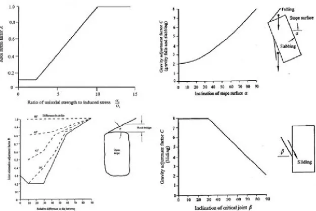
The stability number is derived from modified tunneling quality index Q’ by Barton (Barton, 1974), which is then multiplied by factors A (rock stress factor), B (joint orientation adjustment factor) and C (gravity adjustment factor). Criteria for these factors can be seen in Figure 3.11.
In the analysis two different Q’ will be used: 1,4 for the weak rock mass and 6,8 for the moderate rock mass. When defining the rock stress factor, the UCSs for these categories are 89 MPa and 132 MPa. In most cases this results in A factors 0,1 for the roof and the end walls except bit higher values for end walls at 500m level. As the side walls (HW and FW) are relaxed, they receive A factor value of 0,7 (Stewart & Trueman, 2004). The joint orientation factor is set 0,3 for all surfaces (joints parallel to surface). The gravity adjustment factor C is 8 for the end walls and 2 for the roof and side walls.
26
Figure 3.11 Supporting diagrams for stability graph (Clark & Pakalnis, 1997)
3.4.2 Results
Using the parameters defined in the previous chapter, the stability numbers for the surfaces can be calculated. Results can be seen in the Table 3.4. The variation in the end walls is due to difference in induced stresses in different in-situ stresses.
Moderate Weak Roof 0,4 0,1 End walls 1,6-5,3 0,3-0,6 Side walls 2,8 0,6
Table 3.4 N’ for stope surfaces for moderate and weak rock mass
From the stability graph maximum hydraulic radii for these N’ values can be obtained. The results are that all the roofs up to 10m wide are within the “stable with support” -area and all the end walls in the “stable” –-area. Hydraulic radius can be used to calculate the possible stope lengths. Maximum stope lengths with stable side walls are presented inTable 3.5 Maximum stable side wall lengths.
Stope Height
Maximum stope length
Moderate Weak
30m 20m 12,5m
25m 23m 14m
20m 30m 17m
27
Based on these results it is not suggested to increase the length of the stopes from the current 15m. It could be done in the moderate rock mass, but even though the quality gets better deeper, the weak rock still makes up about 13% of the stopes in deeper parts of Suuri and Roura.
The different in-situ stress combinations have no effect on stope stabilities on 1000m level in stability graph analysis, since even with the lowest estimations end walls and roof receive stress factor A of 0,1 and side walls always receive 0,7.
3.5
Discussion
The stability graph is like other empirical methods, it works best on the area where most of the cases studied are located. In stability graph most of stopes used for the study had larger dimensions than what was examined in this thesis and were located in rock with better quality than what is found in Kittilä mine. Numerical models do not depend on the scale of the excavations, but they take poorly into account the effect of joints, faults and graphitic zones.
28
4
Dilution Control
4.1
Definition of Dilution
Dilution refers to material below cutoff grade that gets blended with ore, thus reducing the grade of excavated material. Dilution in general is impossible to avoid in stoping due to geometries of the orebodies and it is therefore divided into planned and unplanned dilution. Planned dilution is the waste material that is necessary to extract the ore. The unplanned dilution is waste material that originates from outside the stope boundaries. This can be seen in the Figure 4.1.
Figure 4.1 Planned and unplanned dilution (Mitri, et al., 2010)
Dilution can also be defined in few different ways depending on what the information is used on. When estimating plant feed or monitoring production over longer periods of time, it makes most sense to compare the ratio of waste and ore. However, this may not be the best way to express dilution when evaluating the success of stoping. If comparing only the ratio of waste and ore, even terribly failed stope can have low dilution if collapsed material happens to be ore from adjacent stopes.
One way to quantify dilution is ELOS (Equivalent Linear Overbreak Sloughing), which indicates the volume of material from outside the stope boundaries from FW and HW divided by the area of particular wall, seen in Figure 4.2. This is a good way to examine success of stoping as it is not dependent on the volume of the stope, only the surface area of the walls. ELOS can be calculated using the following formula:
29
Figure 4.2 Definition of ELOS (Clark & Pakalnis, 1997)
In this thesis several figures for dilution will be used. The definition for terms to be used can be seen in the list below.
• Waste: material from outside the stope boundaries that is not considered as ore, includes backfilling material. Does not include planned dilution.
• Extra ore: material from outside the stope boundaries that has sufficient grade to be considered as ore.
• Ore loss: material from inside stope boundary that cannot be recovered.
• Dilution: percentage of waste in all excavated material.
• ELOS: All the material from outside stope boundaries from HW or FW, includes waste and extra ore.
4.2
Effect on Profitability
The dilution affects profitability in two ways. First is the direct cost from handling more material. Second is the loss in gold production since the capacity of the plant is fixed and with higher dilution less ore will be processed and thus fewer ounces produced. As the waste and ore are difficult to distinguish from each other visually, it is very likely that all the diluting material will go through the processing plant. The relation between dilution and profit can be seen in the Figure 4.3. This figure was calculated using current operating costs, grades, recoveries and gold price.
30
Figure 4.3 Graph showing relation of dilution and revenue
4.3
Current Situation
Currently the unplanned dilution in Kittilä mine is 19%. The average ELOS for HW and FW is 1,2m, this consists all the material outside stope boundaries. Of all the waste around three quarters originates from HW and FW resulting in 14% dilution. The remaining 5% is from the stope roofs, floors, shoulders and backfilling from neighboring stopes. Not all the material from HW and FW is waste, 13% of this is classified as ore. However, this makes up only 21% of all the extra ore. This means that reducing ELOS would have significant reduce in dilution.
From dilution graphs by Clark (Clark, 1998) and Wang (Wang, 2004) and the numerical models it was estimated that the ELOS for 25m high and 15m long stope should be 0,6m. If this ELOS could be achieved it would bring dilution down to 13%. This number was achieved by decreasing the HW and FW dilution while keeping the dilution from other sources constant. The ratio of extra ore to waste in FW and HW is also kept the same.
4.4
Reasons for Dilution
There are many different possible reasons for dilution and usually the dilution is result of these reasons acting together. This makes it difficult to examine the influence of single variable for dilution. Basically the reasons can be divided into three categories: Drill and blast issues, errors in planning and geotechnical issues.
4.4.1 Drill and Blast
Issues in drill and blasting consist of drilling accuracy and powder factor. Drilling accuracy is result from errors in location of collar, wrong inclination, hole deviation and incorrect hole length. The effect of drill and blast issues to dilution is difficult to predict since there is not enough data to compare drilling accuracy and ELOS. Also, the poor performance in drilling can lead the wide variety of results, including poor fragmentation, loss of blast holes, overbreak or underbreak and increase or decrease in spacing/burden. In Figure 4.4 Possible effects of poor drilling accuracy are shown, in blue are the planned blast holes and in red are the blast holes due to possible errors. As these errors can and will cumulate, the symmetry of the blast is no longer what is
-40,00 -20,00 0,00 20,00 40,00 60,00 80,00 100,00 120,00 0 10 20 30 40 50 Pr ofi t (% ) Dilution
31
planned and may lead to dilution or ore loss. The effect of powder factor was not investigated due to lack of information.
Figure 4.4 Possible effects of poor drilling accuracy
4.4.2 Planning
Dilution due to planning means that the stope boundaries are designed so that dilution is almost inevitable. If the stope would have been designed differently the outcome could still be the same in terms of volume excavated, but waste could have been included in internal dilution. There are few aspects where this makes a difference. First is that it distorts statistics by showing higher dilution than what should really be expected. Second and more important is that it might make some stopes unfeasible. If the stope boundaries are increased the grade gets lower and can fall under cutoff grade. This can lead to situation where badly planned stope may seem feasible but results in operating loss as it gets diluted. Decreasing the stope size can lead to ore loss, which is of course not desired.
Stope limits are currently designed differently for transverse and longitudinal stopes. In transverse stopes the width of the stope is defined by burden of the rings and length is set to 15m. This kind of design leads often to box-type stopes, which may not result in the most feasible stope economically, since the stope width is limited to intervals equal to burden. In longitudinal stopes the boundaries of stope come from the limits of ore. This design easily leads to stope limits that cannot be met due to geometry being too complex, leading to dilution or ore losses. Neither of the designs takes into account the geological formations near the boundaries such as joints, faults and shears.
It is difficult to estimate how much effect errors in planning has since distinguishing planning errors from poor performance in drill and blast is hard.
32
Geotechnical reasons include the influence of stresses and the condition of the surrounding rock mass. Failures are usually caused by interaction of these two factors, like relaxation of poor rock. Geotechnical issues goes hand in hand with planning, since with good planning these issues can be overcome, or at least made less severe.
In the numerical modeling it was noted that stope length and height have significant effect on the ELRD of the stope, which indicates more dilution for higher and longer stopes. In Figure 4.5 and Figure 4.6 the ELOS of the stopes are being compared with stope heights and widths. The ELOS in these figures are calculated by comparing the scanned cavities and designed stope limits, example of cavity scan can be seen in Figure 4.7 From the Figure 4.5 it can be noted that as the stope height increases so does ELOS. The ratio of ELOS for different heights is what is predicted in empirical and numerical methods, but the values are higher. Stope lengths are not being examined since vast majority of the stopes are 15m long and there is not enough stopes longer than this to make reasonable comparison. However, the stope width seems to have larger effect on ELOS than what was expected from the numerical models, this can be seen in Figure 4.6.
Figure 4.5 Stope height effect on ELOS, based on mined stopes 0,0 1,0 2,0 3,0 4,0 5,0 6,0 15 25 35 45 ELO S ( m )
33
Figure 4.6 Stope width effect on ELOS, based on mined stopes
To better understand the effects of geotechnical issues, failed HWs and FWs were investigated. The wall was considered as failed when ELOS was over 1m. The investigation was done by comparing stope limits and cavity scans to locate the failures. Example of cavity scan can be seen in Figure 4.7. The failures were later compared with RQDs from boreholes. The total number of failed walls was 60 out of 132 inspected walls. Of the failed walls 19 were HW and 41 FW. Typical locations for failures were related to overcuts, undercuts and backbreak; these can be seen in Figure 4.8.
Figure 4.7 Example of cavity scan of transverse stope limit in brown and cavity scan in yellow (Agnico-Eagle, 2013) 0,0 1,0 2,0 3,0 4,0 5,0 6,0 0,0 5,0 10,0 15,0 20,0 25,0 30,0 35,0 40,0 ELO S ( m )
34
Figure 4.8 Crosscut of stope looking north showing typical origins of dilution in transverse stope shown in red
The draw points are systematically cable bolted which should decrease the amount of dilution from FW undercut. However, there are cases where cable bolts have not been installed or installed but missing face plates. There is no data about whether certain undercut has been bolted or not, so no correlation between bolting and failures can be made. The HW undercut is shotcreted, overcuts are not reinforced. Influence of over- and undercuts could explain the ELOS difference between HW (0,9m average) and FW (1,4m average) since the HW cuts continue shorter distance into the waste and have smaller effect on stability.
Figure 4.9 Comparison of ELOS and RQD of mined stopes
In Figure 4.9 comparison of RQD and ELOS can be seen, there seems to be no clear correlation between the two. However, the RQD values are from block model and
0,0 1,0 2,0 3,0 4,0 5,0 6,0 7,0 0 20 40 60 80 100 ELO S ( m ) RQD
![SMTP Email Sistem [Compatibility Mode]](data:image/gif;base64,R0lGODlhAQABAIAAAP///wAAACH5BAEAAAAALAAAAAABAAEAAAICRAEAOw==)