Advanced Statistics Demystified Algebra Demystified
Anatomy Demystified Astronomy Demystified Biology Demystified
Business Statistics Demystified Calculus Demystified
Chemistry Demystified College Algebra Demystified Differential Equations Demystified Earth Science Demystified
Electronics Demystified Everyday Math Demystified Geometry Demystified
Math Word Problems Demystified Physics Demystified
Physiology Demystified Pre-Algebra Demystified Pre-Calculus Demystified Project Management Demystified Robotics Demystified
Demystified
STEVEN G. KRANTZ
McGRAW-HILL
written permission of the publisher.
0-07-147116-2
The material in this eBook also appears in the print version of this title: 0-07-144025-9.
All trademarks are trademarks of their respective owners. Rather than put a trademark symbol after every occurrence of a trademarked name, we use names in an editorial fashion only, and to the benefit of the trademark owner, with no intention of infringement of the trademark. Where such designations appear in this book, they have been printed with initial caps.
McGraw-Hill eBooks are available at special quantity discounts to use as premiums and sales promotions, or for use in corporate training programs. For more information, please contact George Hoare, Special Sales, at [email protected] or (212) 904-4069.
TERMS OF USE
This is a copyrighted work and The McGraw-Hill Companies, Inc. (“McGraw-Hill”) and its licensors reserve all rights in and to the work. Use of this work is subject to these terms. Except as permitted under the Copyright Act of 1976 and the right to store and retrieve one copy of the work, you may not decompile, disassemble, reverse engineer, reproduce, modify, create derivative works based upon, transmit, distribute, disseminate, sell, publish or sublicense the work or any part of it without McGraw-Hill’s prior consent. You may use the work for your own noncommercial and personal use; any other use of the work is strictly prohibited. Your right to use the work may be terminated if you fail to comply with these terms.
THE WORK IS PROVIDED “AS IS.” McGRAW-HILL AND ITS LICENSORS MAKE NO GUARANTEES OR WARRANTIES AS TO THE ACCURACY, ADEQUACY OR COMPLETENESS OF OR RESULTS TO BE OBTAINED FROM USING THE WORK, INCLUDING ANY INFORMATION THAT CAN BE ACCESSED THROUGH THE WORK VIA HYPERLINK OR OTHERWISE, AND EXPRESSLY DISCLAIM ANY WARRANTY, EXPRESS OR IMPLIED, INCLUDING BUT NOT LIMITED TO IMPLIED WARRANTIES OF MERCHANTABILITY OR FITNESS FOR A PARTICULAR PURPOSE. McGraw-Hill and its licensors do not warrant or guarantee that the functions contained in the work will meet your requirements or that its operation will be uninterrupted or error free. Neither McGraw-Hill nor its licensors shall be liable to you or anyone else for any inaccuracy, error or omission, regardless of cause, in the work or for any damages resulting therefrom. McGraw-Hill has no responsibility for the content of any information accessed through the work. Under no circumstances shall McGraw-Hill and/or its licensors be liable for any indirect, incidental, special, punitive, consequential or similar damages that result from the use of or inability to use the work, even if any of them has been advised of the possi-bility of such damages. This limitation of liapossi-bility shall apply to any claim or cause whatsoever whether such claim or cause arises in contract, tort or otherwise.
We hope you enjoy this
McGraw-Hill eBook! If
you’d like more information about this book,
its author, or related books and websites,
please
click here.
CONTENTS
Preface
ix
CHAPTER 1
What Is a Differential Equation?
1
1.1
Introductory Remarks
1
1.2
The Nature of Solutions
4
1.3
Separable Equations
7
1.4
First-Order Linear Equations
10
1.5
Exact Equations
13
1.6
Orthogonal Trajectories and Families
of Curves
19
1.7
Homogeneous Equations
22
1.8
Integrating Factors
26
1.9
Reduction of Order
30
1.10 The Hanging Chain and Pursuit Curves 36
1.11 Electrical Circuits
43
Exercises
46
CHAPTER 2
Second-Order Equations
48
2.1
Second-Order Linear Equations with
Constant Coefficients
48
2.2
The Method of Undetermined
Coefficients
54
2.3
The Method of Variation of Parameters 58
2.4
The Use of a Known Solution to
Find Another
62
2.5
Vibrations and Oscillations
65
2.6
Newton’s Law of Gravitation and
Kepler’s Laws
75
2.7
Higher-Order Linear Equations,
Coupled Harmonic Oscillators
85
Exercises
90
CHAPTER 3
Power Series Solutions and
Special Functions
92
3.1
Introduction and Review of
Power Series
92
3.2
Series Solutions of First-Order
Differential Equations
102
3.3
Second-Order Linear Equations:
Ordinary Points
106
Exercises
113
CHAPTER 4
Fourier Series: Basic Concepts
115
4.1
Fourier Coefficients
115
4.2
Some Remarks About Convergence
124
4.3
Even and Odd Functions: Cosine and
Sine Series
128
4.4
Fourier Series on Arbitrary Intervals
132
4.5
Orthogonal Functions
136
Exercises
139
CHAPTER 5
Partial Differential Equations and
Boundary Value Problems
141
5.1
Introduction and Historical Remarks 141
5.2
Eigenvalues, Eigenfunctions, and
the Vibrating String
144
5.3
The Heat Equation: Fourier’s
Point of View
151
5.4
The Dirichlet Problem for a Disc
156
5.5
Sturm–Liouville Problems
162
CHAPTER 6
Laplace Transforms
168
6.1
Introduction
168
6.2
Applications to Differential
Equations
171
6.3
Derivatives and Integrals of
Laplace Transforms
175
6.4
Convolutions
180
6.5
The Unit Step and Impulse
Functions
189
Exercises
196
CHAPTER 7
Numerical Methods
198
7.1
Introductory Remarks
199
7.2
The Method of Euler
200
7.3
The Error Term
203
7.4
An Improved Euler Method
207
7.5
The Runge–Kutta Method
210
Exercises
214
CHAPTER 8
Systems of First-Order Equations
216
8.1
Introductory Remarks
216
8.2
Linear Systems
219
8.3
Homogeneous Linear Systems with
Constant Coefficients
225
8.4
Nonlinear Systems: Volterra’s
Predator–Prey Equations
233
Exercises
238
Final Exam
241
Solutions to Exercises
271
Bibliography
317
If calculus is the heart of modern science, then differential equations are its guts. All physical laws, from the motion of a vibrating string to the orbits of the plan-ets to Einstein’s field equations, are expressed in terms of differential equations. Classically, ordinary differential equations described one-dimensional phenom-ena and partial differential equations described higher-dimensional phenomphenom-ena. But, with the modern advent of dynamical systems theory, ordinary differential equations are now playing a role in the scientific analysis of phenomena in all dimensions.
Virtually every sophomore science student will take a course in introductory ordinary differential equations. Such a course is often fleshed out with a brief look at the Laplace transform, Fourier series, and boundary value problems for the Laplacian. Thus the student gets to see a little advanced material, and some higher-dimensional ideas, as well.
As indicated in the first paragraph, differential equations is a lovely venue for mathematical modeling and the applications of mathematical thinking. Truly meaningful and profound ideas from physics, engineering, aeronautics, statics, mechanics, and other parts of physical science are beautifully illustrated with differential equations.
We propose to write a text on ordinary differential equations that will be mean-ingful, accessible, and engaging for a student with a basic grounding in calculus
(for example, the student who has studied Calculus Demystified by this author
will be more than ready for Differential Equations Demystified). There will be
many applications, many graphics, a plethora of worked examples, and hun-dreds of stimulating exercises. The student who completes this book will be
ix
ready to go on to advanced analytical work in applied mathematics, engineer-ing, and other fields of mathematical science. It will be a powerful and useful learning tool.
CHAPTER
What Is a
Differential
Equation?
1.1 Introductory Remarks
Adifferential equationis an equation relating some functionf to one or more ofits derivatives. An example is
d2f dx2 +2x
df dx +f
2(x)
=sinx. (1)
Observe that this particular equation involves a functionf together with its first
and second derivatives. The objective in solving an equation like(1)is tofind the
1
function f. Thus we already perceive a fundamental new paradigm: When we solve an algebraic equation, we seek a number or perhaps a collection of numbers;
but when we solve a differential equation we seek one or morefunctions.
Many of the laws of nature—in physics, in engineering, in chemistry, in biology, and in astronomy—find their most natural expression in the language of differential equations. Put in other words, differential equations are the language of nature. Applications of differential equations also abound in mathematics itself, especially in geometry and harmonic analysis and modeling. Differential equations occur in economics and systems science and other fields of mathematical science.
It is not difficult to perceive why differential equations arise so readily in the
sciences. Ify =f (x)is a given function, then the derivativedf/dxcan be
inter-preted as the rate of change off with respect tox. In any process of nature, the
variables involved are related to their rates of change by the basic scientific princi-ples that govern the process—that is, by the laws of nature. When this relationship is expressed in mathematical notation, the result is usually a differential equation. Certainly Newton’s Law of Universal Gravitation, Maxwell’s field equations, the motions of the planets, and the refraction of light are important physical examples which can be expressed using differential equations. Much of our understanding of nature comes from our ability to solve differential equations. The purpose of this book is to introduce you to some of these techniques.
The following example will illustrate some of these ideas. According to Newton’s
second law of motion, the accelerationa of a body of massmis proportional to
the total forceF acting on the body. The standard implementation of this
relation-ship is
F =m·a. (2)
Suppose in particular that we are analyzing a falling body of massm. Express
the height of the body from the surface of the Earth asy(t ) feet at time t. The
only force acting on the body is that due to gravity. Ifg is the acceleration due
to gravity (about−32 ft/sec2near the surface of the Earth) then the force exerted
on the body ism·g. And of course the acceleration isd2y/dt2. Thus Newton’s
law (2) becomes
m·g=m·d
2y
dt2 (3)
or
g= d
2y
dt2.
We may make the problem a little more interesting by supposing that air exerts
then the total force acting on the body ismg−k·(dy/dt ). Then the equation(3)
becomes
m·g−k·dy dt =m·
d2y
dt2. (4)
Equations(3)and(4)express the essential attributes of this physical system.
A few additional examples of differential equations are these:
(1−x2)d
2y
dx2 −2x
dy
dx +p(p+1)y =0; (5)
x2d
2y
dx2 +x
dy dx +(x
2
−p2)y =0; (6)
d2y
dx2 +xy=0; (7)
(1−x2)y′′−xy′+p2y =0; (8)
y′′−2xy′+2py =0; (9)
dy
dx =k·y. (10)
Equations (5)–(9) are called Legendre’s equation, Bessel’s equation, Airy’s equation, Chebyshev’s equation, and Hermite’s equation respectively. Each has a vast literature and a history reaching back hundreds of years. We shall touch on each of these equations later in the book. Equation (10) is the equation of exponential decay (or of biological growth).
Math Note: A great many of the laws of nature are expressed as second-order differential equations. This fact is closely linked to Newton’s second law,
which expresses force as mass time acceleration (and acceleration is a second
derivative). But some physical laws are given by higher-order equations. The Euler–Bernoulli beam equation is fourth-order.
Each of equations (5)–(9) is of second-order, meaning that the highest deriva-tive that appears is the second. Equation (10) is of first-order, meaning that the
highest derivative that appears is the first. Each equation is anordinary
differen-tial equation, meaning that it involves a function of a single variable and the
1.2 The Nature of Solutions
An ordinary differential equation of ordernis an equation involving an unknown
functionf together with its derivatives
df dx,
d2f dx2, . . . ,
dnf dxn.
We might, in a more formal manner, express such an equation as
F
x, y,df dx,
d2f dx2, . . . ,
dnf dxn
=0.
How do we verify that a given functionfis actually the solution of such an equation?
The answer to this question is best understood in the context of concrete examples.
e.g. EXAMPLE 1.1
Consider the differential equation
y′′−5y′+6y =0.
Without saying how the solutions are actuallyfound, we can at least check that
y1(x)=e2x andy2(x)=e3xare both solutions.
To verify this assertion, we note that
y1′′−5y1′ +6y1 =2·2·e2x −5·2·e2x+6·e2x
= [4−10+6] ·e2x
≡0
and
y2′′−5y2′ +6y2 =3·3·e3x −5·3·e3x+6·e3x
= [9−15+6] ·e3x
≡0.
This process, of verifying that afunctionis a solution of the given differential
equation, is most likely entirely new for you. You will want to practice and become accustomed to it. In the last example, you may check that any function of the form
y(x)=c1e2x +c2e3x (1)
Math Note: This last observation is an instance of the principle of superposition in physics. Mathematicians refer to the algebraic operation in equation (1) as “taking a linear combination of solutions” while physicists think of the process as superimposing forces.
An important obverse consideration is this: When you are going through the procedure to solve a differential equation, how do you know when you are finished? The answer is that the solution process is complete when all derivatives have
been eliminated from the equation. For then you will haveyexpressed in terms of
x(at least implicitly). Thus you will have found the sought-after function.
For a large class of equations that we shall study in detail in the present book, we will find a number of “independent” solutions equal to the order of the differential equation. Then we will be able to form a so-called “general solution” by combining them as in (1). Of course we shall provide all the details of this process in the development below.
You Try It: Verify that each of the functions y1(x) = ex y2(x) = e2x and
y3(x)=e−4x is a solution of the differential equation
d3y dx3 +
d2y dx2 −10
dy
dx +8y =0.
More generally, check thaty(x) = c1ex +c2e2x +c3e−4x (wherec1, c2, c3 are
arbitrary constants) is a “general solution” of the differential equation.
Sometimes the solution of a differential equation will be expressed as an
implicitly defined function. An example is the equation
dy
dx =
y2
1−xy, (2)
which has solution
xy =lny+c. (3)
Equation (3) represents a solution because all derivatives have been eliminated. Example 1.2 below contains the details of the verification that (3) is the solution of (2).
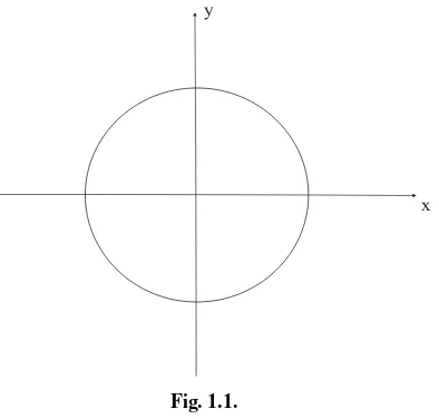
Math Note: It takes some practice to get used to the idea that an implicitly defined function is still a function. A classic and familiar example is the equation
y
x
Fig. 1.1.
This relation expresses y as a function of x at most points. Refer to Fig. 1.1.
In fact the equation (4) entails
y = +1−x2
whenyis positive and
y = −1−x2
when y is negative. It is only at the exceptional points (−1,0) and (−1,0),
where the tangent lines are vertical, that y cannot be expressed as a function
ofx.
Note here that the hallmark of what we call asolutionis that it has no derivatives
in it: it is a straightforward formula, relatingy (the dependent variable) tox (the
independent variable).
e.g. EXAMPLE 1.2
To verify that (3) is indeed a solution of (2), let us differentiate:
d
dx[xy] = d
dx[lny+c],
hence
1·y+x·dy
dx =
or
dy dx
1
y −x
=y.
In conclusion,
dy
dx =
y2
1−xy,
as desired.
One unifying feature of the two examples that we have now seen of verifying
solutions is this: When we solve an equation of ordern, we expectn“independent
solutions” (we shall have to say later just what this word “independent” means)
and we expectnundetermined constants. In the first example, the equation was
of order 2 and the undetermined constants werec1 andc2. In the second example,
the equation was of order 1 and the undetermined constant wasc.
You Try It: Verify that the equationxsiny = cosy gives an implicit solution to the differential equation
dy
dx [xcoty+1]= −1.
1.3 Separable Equations
In this section we shall encounter our first general class of equations with theproperty that
(i) We can immediately recognize members of this class of equations.
(ii) We have a simple and direct method for (in principle)1 solving such
equations.
This is the class ofseparable equations.
DEFINITION 1.1
An ordinary differential equation is separableif it is possible, by elementary
algebraic manipulation, to arrange the equation so that all the dependent
vari-ables (usually they variable) are on one side and all the independent variables
1We throw in this caveat because it can happen, and frequently does happen, that we can write down integrals
(usually thexvariable) are on the other side. The corresponding solution
tech-nique is calledseparation of variables.
Let us learn the method by way of some examples.
e.g. EXAMPLE 1.3
Solve the ordinary differential equation
y′ =2xy.
SOLUTION
In the method of separation of variables—which is a method for first-order
equations only—it is useful to write the derivative using Leibniz notation. Thus we have
dy
dx =2xy.
We rearrange this equation as
dy
y =2x dx.
[It should be noted here that we use the shorthanddyto stand for dy
dxdx.]
Now we can integrate both sides of the last displayed equation to obtain
dy
y =
2x dx.
We are fortunate in that both integrals are easily evaluated. We obtain
lny =x2+c.
[It is important here that we include the constant of integration. We combine the constant from the left-hand integral and the constant from the right-hand integral
into a single constantc.] Thus
y =ex2+c.
We may abbreviateecbyDand rewrite this last equation as
Notice two important features of our final representation for the solution:
(i) We have re-expressed the constantecas the positive constantD.
(ii) Our solution contains one free constant, as we may have anticipated since
the differential equation is of order 1.
We invite you to verify that the solution in equation (1) actually satisfies the original differential equation.
e.g.
EXAMPLE 1.4
Solve the differential equation
xy′ =(1−2x2)tany.
SOLUTION
We first write the equation in Leibniz notation. Thus
x·dy
dx =(1−2x
2)tany.
Separating variables, we find that
coty dy =
1
x −2x
dx.
Applying the integral to both sides gives
coty dy = 1
x −2x
dx
or
ln siny =lnx−x2+C.
Again note that we were careful to include a constant of integration. We may express our solution as
siny =elnx−x2+C
or
siny =D·x·e−x2.
The result may be written as
y=sin−1D·x·e−x2.
Math Note: It should be stressed that not all ordinary differential equations are separable. As an instance, the equation
x2y+y2x =sin(xy)
cannotbe separated so that all thex’s are on one side of the equation and all the
y’s on the other side.
☞
You Try It: Use the method of separation of variables to solve the differential equationx3y′=y.
1.4 First-Order Linear Equations
Another class of differential equations that is easily recognized and readily solved (at least in principle) is that of first-order linear equations.
DEFINITION 1.2
An equation is said to befirst-order linearif it has the form
y′+a(x)y=b(x). (1)
The “first-order” aspect is obvious: only first derivatives appear in the equa-tion. The “linear” aspect depends on the fact that the left-hand side involves a differential operator that acts linearly on the space of differentiable functions.
Roughly speaking, a differential equation is linear ifyand its derivatives are not
multiplied together, not raised to powers, and do not occur as the arguments of functions. This is an advanced idea that we shall explicate in detail later. For now, you should simply accept that an equation of the form (1) is first-order linear, and that we will soon have a recipe for solving it.
As usual, we explicate the method by proceeding directly to the examples.
e.g. EXAMPLE 1.5
Consider the differential equation
y′+2xy=x.
SOLUTION
This equation is plainly not separable (try it and convince yourself that this is so). Instead we endeavor to multiply both sides of the equation by some function that will make each side readily integrable. It turns out that there is a trick that
always works: You multiply both sides bye a(x) dx.
Like many tricks, this one may seem unmotivated. But let us try it out and see how it works in practice. Now
a(x) dx =
2x dx=x2.
[At this point wecouldinclude a constant of integration, but it is not necessary.]
Thuse a(x) dx =ex2. Multiplying both sides of our equation by this factor gives
ex2·y′+ex2·2xy=ex2·x
or
ex2·y
′
=x·ex2.
It is the last step that is a bit tricky. For a first-order linear equation, it is
guaranteedthat if we multiply through bye a(x) dx then the left-hand side of
the equation will end up being the derivative of[e a(x) dx·y]. Now of course
we integrate both sides of the equation:
ex2·y ′
dx=
x·ex2dx.
We can perform both the integrations: on the left-hand side we simply apply the fundamental theorem of calculus; on the right-hand side we do the integration. The result is
ex2·y = 1
2 ·e
x2
+C
or
y = 1
2 +Ce
−x2.
Math Note: Of course not all ordinary differential equations are first order linear. The equation
[y′]2−y =sinx
is indeed first order—because the highest derivative that appears is the first
derivative. But it is nonlinear because the function y′ is multiplied by itself.
The equation
y′′·y−y′=ex
is second order and is also nonlinear—becausey′′is multiplied timesy.
Summary of the method of first-order
linear equations
To solve a first-order linear equation
y′+a(x)y=b(x),
multiply both sides of the equation by the “integrating factor”e a(x) dx and then
integrate.
e.g. EXAMPLE 1.6
Solve the differential equation
x2y′+xy=x2·sinx.
SOLUTION
First observe that this equation is not in the standard form (equation (1)) for
first-order linear. We render it so by multiplying through by a factor of 1/x2.
Thus the equation becomes
y′+ 1
xy =sinx.
Nowa(x) = 1/x, a(x) dx =ln|x|, ande a(x) dx = |x|. We multiply the differential equation through by this factor. In fact, in order to simplify the
calculus, we shall restrict attention tox >0. Thus we may eliminate the absolute
value signs. Thus
Now, as is guaranteed by the theory, we may rewrite this equation as
x·y′ =x·sinx.
Applying the integral to both sides gives
x·y′dx=
x·sinx dx.
As usual, we may use the fundamental theorem of calculus on the left, and we may apply integration by parts on the right. The result is
x·y = −x·cosx+sinx+C.
We finally find that our solution is
y= −cosx+sinx
x +
C x.
You should plug this answer into the differential equation and check that it works.
You Try It: Use the method of first-order linear equations to find the complete solution of the differential equation
y′+ 1 xy =e
x.
1.5 Exact Equations
A great many first-order equations may be written in the formM(x, y) dx+N (x, y) dy=0. (1)
This particular format is quite suggestive, for it brings to mind a family of curves.
Namely, if it happens that there is a functionf (x, y)so that
∂f
∂x =M and
∂f
∂y =N, (2)
then we can rewrite the differential equation as
∂f ∂x dx+
∂f
Of course the only way that such an equation can hold is if
∂f
∂x ≡0 and
∂f ∂y ≡0.
And this entails that the functionf be identically constant. In other words,
f (x, y)≡c.
This last equation describes a family of curves: for each fixed value ofc, the
equation expressesyimplicitly as a function ofx, and hence gives a curve. In later
parts of this book we shall learn much from thinking of the set of solutions of a differential equation as a smoothly varying family of curves in the plane.
The method of solution just outlined is called the method of exact equations.
It depends critically on being able to tell when an equation of the form(1)can be
written in the form(3). This in turn begs the question of when(2)will hold.
Fortunately, we learned in calculus a complete answer to this question. Let us review the key points. First note that, if it is the case that
∂f
∂x =M and
∂f
∂y =N, (4)
then we see (by differentiation) that
∂2f
∂y∂x =
∂M
∂y and
∂2f
∂x∂y =
∂N ∂x.
Since mixed partials of a smooth function may be taken in any order, we find that anecessary conditionfor the condition(4)to hold is that
∂M
∂y =
∂N
∂x. (5)
We call (5) theexactness condition. This provides us with a useful test for when
the method of exact equations will apply.
It turns out that condition(5) is also sufficient—at least on a domain with no
holes. We refer you to any good calculus book (see, for instance, [STE]) for the details of this assertion. We will use our worked examples to illustrate the point.
e.g. EXAMPLE 1.7
Use the method of exact equations to solve
x
2 ·coty·
dy
SOLUTION
First, we rearrange the equation as
2xsiny dx+x2cosy dy=0.
Observe that the role ofM(x, y)is played by 2xsinyand the role ofN (x, y)
is played byx2cosy. Next we see that
∂M
∂y =2xcosy = ∂N
∂x.
Thus our necessary condition for the method of exact equations to work is satisfied. We shall soon see that it is also sufficient.
We seek a functionf such that∂f/∂x = M(x, y)= 2xsiny and∂f/∂y =
N (x, y) = x2cosy. Let us begin by concentrating on the first of these conditions:
∂f
∂x =2xsiny,
hence
∂f
∂x dx=
2xsiny dx.
The left-hand side of this equation may be evaluated with the fundamental
theorem of calculus. Treatingxandyas independent variables (which is part of
this method), we can also compute the integral on the right. The result is
f (x, y)=x2siny+φ (y). (6)
Now there is an important point that must be stressed. You should by now have expected a constant of integration to show up. But in fact our “constant
of integration” is φ (y). This is because our integral was with respect to x,
and therefore our constant of integration should be the most general possible
expressionthat does not depend onx. That, of course, would be a function ofy.
Now we differentiate both sides of(6)with respect toyto obtain
N (x, y)= ∂f ∂y =x
2cosy
+φ′(y).
But of course we already know thatN (x, y)=x2cosy. The upshot is that
φ′(y)=0
or
φ (y)=d,
Plugging this information into equation(6)now yields that
f (x, y) =x2siny+d.
We stress that this is not the solution of the differential equation. Before
you proceed, please review the outline of the method of exact equations that preceded this example. Our job now is to set
f (x, y)=c.
So
x2·siny =c, (7)
wherec=c−d.
Equation (7) is in fact the solution of our differential equation, expressed
implicitly. If we wish, we can solve foryin terms ofxto obtain
y=sin−1 c
x2.
And you may check that this is the solution of the given differential equation.
e.g. EXAMPLE 1.8
Use the method of exact equations to solve the differential equation
y2dx−x2dy =0.
SOLUTION
We first test the exactness condition:
∂M
∂y =2y = −2x= ∂N
∂x.
The exactness condition fails. As a result, this ordinary differential equation cannot be solved by the method of exact equations.
Notice that we arenotsaying here that the given differential equation cannot
Math Note: It is an interesting fact that the concept of exactness is closely linked to the geometry of the domain of the functions being studied. An important example is
M(x, y)= −y
x2
+y2, N (x, y)=
x x2
+y2.
We take the domain ofMandN to beU = {(x,y):1< x2+y2 <2}in order to
avoid the singularity at the origin. Of course this domain has a hole.
Then you may check that ∂M/∂y = ∂N/∂x on U. But it can be shown that
there is no functionf (x,y)such that∂f/∂x =Mand∂f/∂y =N. Again, the hole
in the domain is the enemy.
Without advanced techniques at our disposal, it is best when using the method of exact equations to work only on domains that have no holes.
Math Note: It is a fact that, even when a differential equation fails the “exact equations test,” it is always possible to multiply the equation through by an
“integrating factor” so that itwill pass the exact equations test. As an example,
the differential equation
2xysinx dx+x2sinx dy =0
isnot exact. But multiply through by the integrating factor 1/sinx and the new
equation
2xy dx+x2dy =0
isexact.
Unfortunately, it can be quite difficult to discover explicitly what that integrating factor might be. We will learn more about the method of integrating factors in Section 1.8.
e.g.
EXAMPLE 1.9
Use the method of exact equations to solve
eydx+(xey +2y) dy =0.
SOLUTION
First we check for exactness:
∂M
∂y =
∂ ∂y[e
y
] =ey = ∂ ∂x[xe
y
+2y] = ∂M ∂x .
Now we can proceed to solve forf:
∂f
∂x =M =e
y,
hence
f (x, y)=x·ey +φ (y).
But then
∂
∂yf (x, y)= ∂ ∂y
x·ey +φ (y)=x·ey+φ′(y).
And this last expression must equalN (x, y)=xey+2y. It follows that
φ′(y)=2y
or
φ (y)=y2+d.
Altogether, then, we conclude that
f (x, y)=x·ey +y2+d.
We must not forget the final step. The solution of the differential equation is
f (x, y)=c
or
x·ey+y2+d =c
or
x·ey +y2 =c.
This time we must content ourselves with the solution expressed implicitly,
since it is not feasible to solve fory in terms ofx.
☞
You Try It: Use the method of exact equations to solve the differential equation1.6 Orthogonal Trajectories and
Families of Curves
We have already noted that it is useful to think of the collection of solutions of afirst-order differential equations as a family of curves. Refer, for instance, to the last example of the preceding section. We solved the differential equation
eydx+(xey+2y) dy=0
and found the solution set
x·ey+y2 =c. (1)
For each value ofc, the equation describes a curve in the plane.
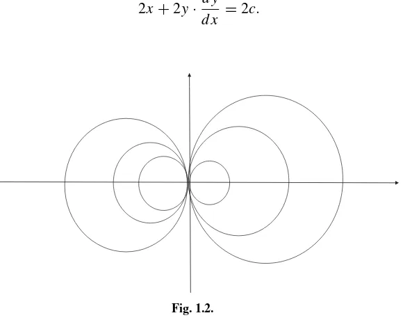
Conversely, if we are given a family of curves in the plane then we can pro-duce a differential equation from which the curves come. Consider the example of the family
x2+y2 =2cx. (2)
You can readily see that this is the family of all circles tangent to they-axis at the
origin (Fig. 1.2).
We may differentiate the equation with respect tox, thinking ofy as a function
ofx, to obtain
2x+2y·dy
dx =2c.
Now the original equation(2)tells us that
x+y
2
x =2c,
and we may equate the two expressions for the quantity 2c (the point being to
eliminate the constantc). The result is
2x+2y·dy
dx =x+ y2
x
or
dy
dx =
y2−x2
2xy . (3)
In summary, we see that we can pass back and forth between a differential equation and its family of solution curves.
There is considerable interest, given a family F of curves, to find the
corre-sponding familyGof curves that are orthogonal (or perpendicular) to those ofF.
For instance, ifF represents the flow curves of an electric current, thenGwill be
the equipotential curves for the flow. If we bear in mind that orthogonality of curves means orthogonality of their tangents, and that orthogonality of the tangent lines means simply that their slopes are negative reciprocals, then it becomes clear what we must do.
e.g. EXAMPLE 1.10
Find the orthogonal trajectories to the family of curves
x2+y2 =c.
SOLUTION
First observe that we can differentiate the given equation to obtain
2x+2y·dy
dx =0.
The constantchas disappeared, and we can take this to be the differential
equa-tion for the given family of curves (which in fact are all the circles centered at the origin—see Fig. 1.3).
We rewrite the differential equation as
dy
dx = −
Fig. 1.3.
Now taking negative reciprocals, as indicated in the discussion right before this example, we obtain the new differential equation
dy
dx =
y x.
We may easily separate variables to obtain
1
ydy =
1
x dx.
Applying the integral to both sides yields
1
y dy=
1
x dx
or
ln|y| =ln|x| +C.
With some algebra, this simplifies to
|y| =D|x|
or
y = ±Dx.
Fig. 1.4.
Math Note: It is not the case that an “arbitrary” family of curves will have
well-defined orthogonal trajectories. Consider, for example, the curves y = |x| +c
and think about why the orthogonal trajectories for these curves might lead to confusion.
☞
You Try It: Find the orthogonal trajectories to the curvesy =x2+c.1.7 Homogeneous Equations
You should be cautioned that the word “homogeneous” has two meanings in this subject (as mathematics is developed simultaneously by many people all over the world, and they do not always stop to cooperate on their choices of terminology).
One usage, which we shall see and use frequently later in the book, is that an
ordinary differential equation is homogeneous when the right-hand side is zero;
that is, there is no forcing term.
The other usage will be relevant to the present section. It bears on the “balance” of weight among the different variables. It turns out that a differential equation
in which thex andy variables have a balanced presence is amenable to a useful
First of all, a functiong(x, y) of two variables is said to behomogeneous of degreeα, forαa real number, if
g(t x, ty)=tαg(x, y) for allt >0.
As examples, consider:
• Letg(x, y)=x2+xy. Theng(t x, ty)=t2·g(x, y), sogis homogeneous of degree 2.
• Letg(x, y) = sin[x/y]. Theng(t x, ty) = g(x, y) = t0·g(x, y), sog is homogeneous of degree 0.
• Letg(x, y)=x2+y2. Theng(t x, ty)=t·g(x, y), sogis homogeneous
of degree 1.
In case a differential equation has the form
M(x, y) dx+N (x, y) dy=0
andM, Nhave thesame degree of homogeneity, then it is possible to perform the
change of variablez = y/x and make the equation separable (see Section 1.3).
Of course we then have a well-understood method for solving the equation. The next examples will illustrate the method.
e.g.
EXAMPLE 1.11
Use the method of homogeneous equations to solve the equation
(x+y) dx−(x−y) dy =0.
SOLUTION
First notice that the equation isnot exact, so we must use some other method to
find a solution. Now observe thatM(x, y) = x+y andN (x, y) = −(x −y)
and each is homogeneous of degree 1. We thus rewrite the equation in the form
dy
dx =
x+y x−y.
Dividing numerator and denominator byx, we finally have
dy
dx =
1+y
x
1−y
x
. (1)
The point of these manipulations is that the right-hand side is now plainly homogeneous of degree 0. We introduce the change of variable
z= y
hence
y =zx
and
dy
dx =z+x· dz
dx. (3)
Putting (2) and (3) into (1) gives
z+xdz
dx =
1+z
1−z.
Of course this may be rewritten as
xdz
dx =
1+z2
1−z
or
1−z
1+z2 dz=
dx x .
We apply the integral, and rewrite the left-hand side, to obtain
dz
1+z2 −
z dz
1+z2 =
dx
x .
The integrals are easily evaluated, and we find that
tan−1z−1
2ln(1+z
2)
=lnx+C.
Now we return to our original notation by settingz=y/x. The result is
tan−1y
x −ln
x2+y2 =C.
Thus we have expressedyimplicitly as a function ofx, and thereby solved the
differential equation.
Math Note: Of course it should be clearly understood that most functions are
nothomogeneous. The functions
• f (x, y)=x+y2
• f (x, y)=xsiny
• f (x, y)=exy
• f (x, y)=log(x2y)
e.g.
EXAMPLE 1.12
Solve the differential equation
xy′ =2x+3y.
SOLUTION
It is plain that the equation is first-order linear, and we encourage the reader to solve the equation by that method for practice and comparison purposes. Instead, developing the ideas of the present section, we will use the method of homogeneous equations.
If we rewrite the equation as
−(2x+3y) dx+x dy=0,
then we see that each ofM = −(2x +3y) and N = x is homogeneous of
degree 1. Thus we have as
dy
dx =
2x+3y
x .
The right-hand side is homogeneous of degree 0, as we expect.
We setz=y/xanddy/dx =z+x[dz/dx]. The result is
z+x· dz
dx =2+3 y
x =2+3z.
The equation separates, as we anticipate, into
dz
2+2z =
dx x .
This is easily integrated to yield
1
2ln(1+z)=lnx+C
or
z=Dx2−1.
Resubstitutingz=y/x gives
y
x =Dx
2
−1,
hence
y =Dx3−x.
☞
You Try It: Use the method of homogeneous equations to solve the differential equation(y2−x2) dx+xy dy=0.
1.8 Integrating Factors
We used a special type of integrating factor in Section 1.4 on first-order linear equations. At that time, we suggested that integrating factors may be applied in some generality to the solution of first-order differential equations. The trick is in
findingthe integrating factor.
In this section we shall discuss this matter in some detail, and indicate the uses and the limitations of the method of integrating factors.
First let us illustrate the concept of integrating factor by way of a concrete example.
e.g. EXAMPLE 1.13
The differential equation
y dx+(x2y−x) dy =0 (1)
is plainlynot exact, just because∂M/∂y = 1 while ∂N/∂x = 2xy−1, and
these are unequal. However, if we multiply the equation(1)through by a factor
of 1/x2, then we obtain the equivalent equation
y x2 dx+
y−1
x
=0,
and this equationis exact(as you may easily verify by calculating∂M/∂yand
∂N/∂x). And of course we have a direct method (see Section 1.5) for solving such an exact equation.
We call the function 1/x2in this last example anintegrating factor. It is obviously
a matter of some interest to be able to find an integrating factor for any given first-order equation. So, given a differential equation
M(x, y) dx+N (x, y) dy=0,
we wish to find a functionµ(x, y)such that
is exact. This entails
∂(µ·M)
∂y =
∂(µ·N )
∂x .
Writing this condition out, we find that
µ∂M
∂y +M
∂µ
∂y =µ
∂N
∂x +N
∂µ ∂x.
This last equation may be rewritten as
1
µ
N∂µ
∂x −M
∂µ ∂y
= ∂M∂y −∂N∂x.
Now we use the method of wishful thinking: we suppose not only that an
inte-grating factorµexists, but in fact that one exists that only depends on the variable
x(and not at all ony). Then the last equation reduces to
1
µ dµ
dx =
∂M/∂y−∂N/∂x
N .
Notice that the left-hand side of this new equation is a function ofx only. Hence
so is the right-hand side. Call the right-hand sideg(x). Notice thatgis something
that we can always compute. Thus
1
µ dµ
dx =g(x),
hence
d(lnµ)
dx =g(x)
or
lnµ=
g(x) dx.
We conclude that, in case there is an integrating factor µ that depends on x
only, then
µ(x)=e g(x) dx,
where
g(x)= ∂M
∂y −
∂N ∂x
can always be computed directly from the original differential equation.
e.g. EXAMPLE 1.14
Solve the differential equation
(xy−1) dx+(x2−xy) dy =0.
SOLUTION
You may plainly check that this equation is not exact. It is also not separable.
So we shall seek an integrating factor that depends only onx. Now
g(x)= ∂M/∂y−∂N/∂x
N =
[x] − [2x−y]
x2−xy = −
1
x.
Thisg depends only on x, signaling that the methodology we just developed
will actually work. We set
µ(x)=e g(x) dx =e −1/x dx = 1 x.
This is our integrating factor. We multiply the original differential equation
through by 1/xto obtain
y− 1
x
dx+(x−y) dy =0.
You may check thatthisequation is certainly exact. We omit the details of solving
this exact equation, since that methodology was covered in Section 1.5.
Of course the roles ofyandxmay be reversed in our reasoning for finding an
integrating factor. In case the integrating factorµdepends only ony(and not at all
onx) then we set
h(y)= −∂M/∂y−∂N/∂x
M
and define
µ(y)=e h(y) dy.
e.g. EXAMPLE 1.15
Solve the differential equation
SOLUTION
First observe that the equation is not exact as it stands. Second,
∂M/∂y−∂N/∂x
N =
−1
2x−yey
doesnotdepend only onx. So instead we look at
−∂M/∂yM−∂N/∂x = −−y1,
and this expression depends only ony. So it will be ourh(y). We set
µ(y)=e h(y) dy =e 1/y dy=y.
Multiplying the differential equation through byµ(y)=y, we obtain the new
equation
y2dx+(2xy−y2ey) dy=0.
You may easily check that this new equation is exact, and then solve it by the method of Section 1.5.
You Try It: Use the method of integrating factors to transform the differential equation
2y x2 dx+
1
x dy=0
to an exact equation. Then solve it.
Math Note: We conclude this section by noting that the differential equation
xy3dx+yx2dy =0
has the properties that
• It is not exact;
• ∂M/∂y−∂N/∂x
N does not depend onx only;
• −∂M/∂y−∂N/∂x
M does not depend onyonly.
1.9 Reduction of Order
Later in the book, we shall learn that virtuallyanyordinary differential equation can
be transformed to a first-ordersystemof equations. This is, in effect, just a notational
trick, but it emphasizes the centrality of first-order equations and systems. In the present section, we shall learn how to reduce certain higher-order equations to first-order equations—ones which we can frequently solve.
In each differential equation in this section,x will be the independent variable
and y the dependent variables. So a typical second-order equation will involve
x, y, y′, y′′. The key to the success of each of the methods that we shall introduce in this section is that one variable must be missing from the equation.
1.9.1 DEPENDENT VARIABLE MISSING
In case the variable y is missing from our differential equation, we make the
substitutiony′=p. This entailsy′′=p′. Thus the differential equation is reduced
to first-order.
e.g. EXAMPLE 1.16
Solve the differential equation
xy′′−y′ =3x2
using reduction of order.
SOLUTION
We sety′=pandy′′=p′, so that the equation becomes
xp′−p=3x2.
Observe that this new equation is first-order linear in the new dependent
variablep. We write it in standard form as
p′− 1
xp=3x.
We may solve this equation by using the integrating factorµ(x)=e −1/x dx =
1/x. Thus
1
xp
′− 1
so
1
xp ′
=3
or
1
xp ′
dx=
3dx.
Performing the integrations, we conclude that
1
xp =3x+C,
hence
p(x)=3x2+Cx.
Now we recall thatp =y′, so we make that substitution. The result is
y′=3x2+Cx,
hence
y =x3+ C
2x
2
+D=x3+Ex2+D.
We invite you to confirm that this is the complete and general solution to the original differential equation.
e.g.
EXAMPLE 1.17
Find the solution of the differential equation
[y′]2=x2y′′.
SOLUTION
We note thaty is missing, so we make the substitutionp = y′,p′ =y′′. Thus
the equation becomes
p2=x2p′.
This equation is amenable to separation of variables. The result is
dx x2 =
which integrates to
−1
x = −
1
p +E
or
p= 1
E
1− 1
1+Ex
for some unknown constantE. We re-substitutep =y′ and integrate to obtain
finally that
y(x)= x
E −
1
E2 ln(1+Ex)+D
is the general solution of the original differential equation.
Math Note: As usual, notice that the solution of any of our second-order differ-ential equations gives rise to two undetermined constants. Usually these will be specified by two initial conditions.
☞
You Try It: Use the method of reduction of order to solve the differential equationy′′−y′ =x.
1.9.2 INDEPENDENT VARIABLE MISSING
In case the variable x is missing from our differential equation, we make the
substitution y′ = p. This time the corresponding substitution for y′′ will be
a bit different. To wit,
y′′= dp
dx =
dp dy
dy
dx =
dp dy ·p.
This change of variable will reduce our differential equation to first-order. In the
reduced equation, we treatpas the dependent variable (or function) and y as the
e.g.
EXAMPLE 1.18
Solve the differential equation
y′′+k2y =0
[where it is understood thatkis a real constant].
SOLUTION
We notice that the independent variable is missing. So we make the substitution
y′ =p, y′′=p·dp dy.
The equation then becomes
p·dp dy +k
2y
=0.
In this new equation we can separate variables:
p dp = −k2y dy,
hence
p2
2 = −k
2y2
2 +C,
p= ±
D−k2y2 = ±k
E−y2.
Now we re-substitutep =dy/dx to obtain
dy dx = ±k
E−y2.
We can separate variables to obtain
dy
E−y2 = ±k dx,
hence
sin−1 √y
E = ±kx+F
or
y
√
thus
y =√Esin(±kx+F ).
Now we apply the sum formula for sine to rewrite the last expression as
y=√EcosFsin(±kx)+√EsinFcos(±kx).
A moment’s thought reveals that we may consolidate the constants and finally write our general solution of the differential equation as
y=Asin(kx)+Bcos(kx).
We shall learn in the next chapter a different, and perhaps more expeditious, method of attacking examples of the last type. It should be noted quite plainly in the last example, and also in some of the earlier examples of the section, that the method of reduction of order basically transforms the problem of solving one second-order
equation to a new problem of solvingtwofirst-order equations. Examine each of
the examples we have presented and see whether you can say what the two new equations are.
In the next example, we will solve a differential equation subject to aninitial
condition. This will be an important idea throughout the book. Solving a differential
equation gives rise to a familyof functions. Specifying the initial condition is a
natural way to specialize down to a particular solution. In applications, these initial conditions will make good physical sense.
e.g. EXAMPLE 1.19
Use the method of reduction of order to solve the differential equation
y′′=y′·ey
with initial conditionsy(0)=0 andy′(0)=1.
SOLUTION
We make the substitution
y′ =p, y′′=p·dp dy.
So the equation becomes
p·dp
dy =p·e
y.
We of course may separate variables, so the equation becomes
This is easily integrated to give
p=ey+C.
Now we re-substitutep =y′to find that
y′ =ey +C
or
dy dx =e
y
+C.
Because of the initial conditionsy(0)=0 and[dy/dx](0)=1, we may conclude
right away thatC =0. Thus our equation is
dy ey =dx
or
−e−y =x+D.
Of course we can rewrite the equation finally as
y = −ln(−x+E).
Sincey(0)=0, we conclude that
y(x)= −ln(−x+1)
is the solution of our initial value problem.
You Try It: Use the method of reduction of order to solve the differential equation
y′′−y′y =0.
You Try It: Use the method of reduction of order to solve the initial value problem
1.10 The Hanging Chain and
Pursuit Curves
1.10.1 THE HANGING CHAIN
Imagine a flexible steel chain, attached firmly at equal height at both ends, hanging under its own weight (see Fig. 1.5). What shape will it describe as it hangs?
This is a classical problem of mechanical engineering, and its analytical solution involves calculus, elementary physics, and differential equations. We describe it here.
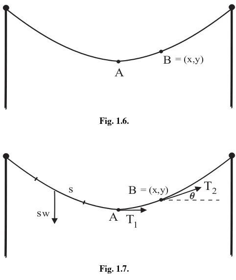
We analyze a portion of the chain between pointsAandB, as shown in Fig. 1.6,
whereAis the lowest point of the chain andB =(x, y)is a variable point. We let
• T1be the horizontal tension atA;
• T2be the component of tensiontangentto the chain atB;
• wbe the weight of the chain per unit of length.
HereT1, T2, ware numbers. Figure 1.7 exhibits these quantities.
Notice that ifs is the length of the chain between two given points, thensw is
the downward force of gravity on this portion of the chain; this is indicated in the
figure. We use the symbolθ to denote the angle that the tangent to the chain atB
makes with the horizontal.
By Newton’s first law we may equate horizontal components of force to obtain
T1=T2cosθ. (1)
Likewise, we equate vertical components of force to obtain
ws=T2sinθ. (2)
A
B = (x,y)
Fig. 1.6.
A
B= (x,y)
w
T
12
T
s s
Fig. 1.7.
Dividing the right side of(2)by the right side of(1)and the left side of(2)by the
left side of(1)and equating gives
ws T1 =
tanθ.
Think of the hanging chain as the graph of a function:yis a function ofx.Theny′
atBequals tanθ, so we may rewrite the last equation as
y′ = ws T1
.
We can simplify this equation by a change of notation: setq =y′.Then we have
q(x)= w T1
s(x). (3)
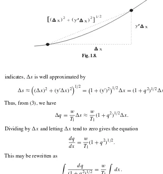
Ifx is an increment ofx, thenq = q(x+x)−q(x)is the
x
y x
( x )2 + ( y x )2
[
[
[
1/2Fig. 1.8.
indicates,sis well approximated by
s ≈(x)2+(y′x)21/2=1+(y′)21/2x =(1+q2)1/2x.
Thus, from(3), we have
q = w
T1
s ≈ w
T1
(1+q2)1/2x.
Dividing byx and lettingxtend to zero gives the equation
dq
dx =
w T1
(1+q2)1/2. (4)
This may be rewritten as
dq
(1+q2)1/2 =
w T1
dx.
It is trivial to perform the integration on the right side of the equation, and a little
extra effort enables us to integrate the left side (use the substitutionu=tanψ, or
else use inverse hyperbolic trigonometric functions). Thus we obtain
sinh−1q = w
T1
x+C.
We know that the chain has a horizontal tangent when x = 0 (this corresponds
to the pointA—Fig. 1.7). Thusq(0) = y′(0) = 0.Substituting this into the last
equation givesC=0.Thus our solution is
sinh−1q(x)= w
T1
or
q(x)=sinh
w T1
x
or
dy
dx =sinh
w T1
x
.
Finally, we integrate this last equation to obtain
y(x)= T1 w cosh
w
T1
x
+D,
whereDis a constant of integration. The constantDcan be determined from the
heighth0of the pointAfrom thex-axis:
h0=y(0)=
T1
w cosh(0)+D,
hence
D=h0−
T1
w.
Our hanging chain is completely described by the equation
y(x)= T1 w cosh
w
T1
x
+h0−
T1
w.
This curve is called acatenary, from the Latin word for chain (catena). Catenaries
arise in a number of other physical problems, including thebrachistochroneand
tautochronewhich are discussed in this book. The St. Louis arch is in the shape of a catenary.
1.10.2 PURSUIT CURVES
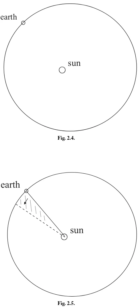
A submarine speeds across the ocean bottom in a particular path, and a destroyer at a remote location decides to engage in pursuit. What path does the destroyer follow? Problems of this type are of interest in a variety of applications. We examine a few examples. The first one is purely mathematical, and devoid of “real world” trappings.
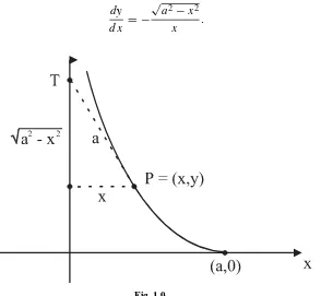
e.g. EXAMPLE 1.20
A pointP is dragged along thex–yplane by a stringP T of fixed lengtha. IfT
begins at the origin and moves along the positivey-axis, and ifP starts at the
point(a,0), then what is the path ofP?
SOLUTION
The curve described byP is called, in the classical literature, atractrix(from
the Latin tractum, meaning “drag”). Figure 1.9 exhibits the salient features
of the problem.
Observe that we can calculate the slope of the pursuit curve at the pointP in
two ways: (i) as the derivative ofywith respect tox, and (ii) as the ratio of sides
of the relevant triangle. This leads to the equation
dy
dx = −
√
a2−x2
x .
This is a separable, first-order differential equation. We write
dy = −
√
a2−x2
x dx.
Performing the integrations (the right-hand side requires the trigonometric
substitutionx=sinψ), we find that
y=aln
a+√a2−x2
x
−a2−x2
is the equation of the tractrix.2
e.g.
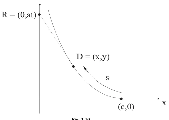
EXAMPLE 1.21
A rabbit begins at the origin and runs up they-axis with speedafeet per second.
At the same time, a dog runs at speedb from the point(c,0)in pursuit of the
rabbit. What is the path of the dog?
SOLUTION
At timet, measured from the instant both the rabbit and the dog start, the rabbit
will be at the pointR=(0, at )and the dog atD=(x, y). We wish to solve for
yas a function ofx. Refer to Fig. 1.10.
The premise of a pursuit analysis is that the line throughDandRis tangent to
the path—that is, the dog will always run straight at the rabbit. This immediately gives the differential equation
dy
dx =
y−at
x .
This equation is a bit unusual for us, sincexandyare both unknown functions
oft. First, we rewrite the equation as
xy′−y = −at.
[Here the′ on y stands for differentiation inx.] We differentiate this equation
with respect tox, which gives
xy′′= −adt dx.
2This curve is of considerable interest in other parts of mathematics. If it is rotated about they-axis, then the result
D = (x,y)
R = (0,at)
s
(c,0)
x
Fig. 1.10.
Sincesis arc length along the path of the dog, it follows thatds/dt =b. Hence
dt
dx =
dt ds ·
ds
dx = −
1
b ·
1+(y′)2;
here the minus sign appears becausesdecreases whenxincreases (see Fig. 1.10).
Combining the last two displayed equations gives
sy′′= a b
1+(y′)2.
For convenience, we set k = a/b, y′ = p, and y′′ = dp/dx (the
lat-ter two substitutions being one of our standard reduction of order techniques). Thus we have
dp
1+p2 =k
dx x .
Now we may integrate, using the conditionp=0 whenx =c. The result is
ln
p+
1+p2
=lnx
c k
.
When we solve forp, we find that
dy
dx =p=
1 2
x
c k
−c
x
k
In order to continue the analysis, we need to know something about the
relative sizes ofa andb. Suppose, for example, thata < b (sok < 1),
mean-ing that the dog will certainly catch the rabbit. Then we can integrate the last equation to obtain
y(x)= 1
2
c k+1
x c
k+1
− c
(1−k) c
x k−1
+D.
Sincey =0 whenx =c, we find thatD =ck. Of course the dog catches the
rabbit whenx = 0. Since both exponents onx are positive, we can setx = 0
and solve fory to obtainy = ck as the point at which the dog and the rabbit
meet.
We invite you to consider what happens whena=band hencek=1.
Math Note: The idea of and analysis of pursuit curves is of great interest to the navy. Battle strategies are devised using these ideas.
1.11 Electrical Circuits
We have alluded elsewhere in the book to the fact that our analyses of vibratingsprings and other mechanical phenomena are analogous to the situation for electrical circuits. Now we shall examine this matter in some detail.
We consider the flow of electricity in the simple electrical circuit exhibited in Fig. 1.11. The elements that we wish to note are these:
A. A source of electromotive force (emf )E—perhaps a battery or generator—
which drives electric charge and produces a currentI. Depending on the
nature of the source,Emay be a constant or a function of time.
B. A resistor of resistanceR, which opposes the current by producing a drop
in emf of magnitude
ER =RI.
This equation is calledOhm’s Law.
C. An inductor of inductanceL, which opposes any change in the current by
producing a drop in emf of magnitude
EL=L·
dI dt.
D. A capacitor (or condenser) of capacitanceC, which stores the chargeQ. The
E
R
I
L
Q
C
Fig. 1.11.
and the drop in emf arising in this way is
EC=
1
C ·Q.
Furthermore, since the current is the rate of flow of charge, and hence the rate at which charge builds up on the capacitor, we have
I = dQ
dt .
Those unfamiliar with the theory of electricity may find it helpful to draw an
analogy here between the currentI and the rate of flow of water in a pipe. The
electromotive forceEplays the role of a pump producing pressure (voltage) that
causes the water to flow. The resistanceR is analogous to friction in the pipe—
which opposes the flow by producing a drop in the pressure. The inductanceLis
a sort of inertia that opposes any change in flow by producing a drop in pressure if the fl