Urban Passenger Travel Demand Indonesia

C H A P T E R S I X T E E N

Urban Passenger

Travel Demand

André de Palma, Robin Lindsey,

and Nathalie Picard

16.1

I

NTRODUCTION

The idea of tolling roads to reduce traffic congestion was suggested back in 1920. For several decades, road pricing was largely dismissed as impractical and pub-licly unacceptable, and early attempts to introduce tolls on urban roads foundered because of poor marketing strategies and political opposition. But a number of road-pricing projects are now in operation or planned around the world, and in the 1990s the US federal government introduced a Value Pricing program to fund innovative road and parking pricing schemes.

This essay reviews two econometric studies of road pricing in the United States. One, by Lam and Small (2001), concerns a toll-lanes project on State Route 91 in Orange County, California, which was the first Value Pricing project to be imple-mented. Lam and Small use data obtained from users of the freeway to estimate individual choice models of whether to drive on the toll lanes and related travel decisions. The second study, by Bhat and Castelar (2002), investigates the effects of hypothetical congestion-pricing initiatives in the San Francisco Bay Area. Their study illustrates how traveler responses to policies that have yet to be implemented can be estimated.

successful. One policy, which was emphasized in the United Kingdom until the 1980s, was to forecast traffic demand and then to add enough road capacity to accommodate it. This “predict and provide” approach was undermined by the tendency – known as induced or latent demand – for new roads or lanes to fill up with traffic generated by new trips or diverted from other routes or times of day. And by encouraging auto travel, “predict and provide” exacerbated auto-related externalities such as emissions and noise. Another policy, which was popular in the USA during the 1960s and 1970s, was to spend heavily on mass transit sys-tems. The systems were generally very expensive, and some attracted far fewer riders than proponents claimed they would. Moreover, some of the riders were drawn away from buses rather than from their cars, so that reductions in auto traffic were even less than ridership statistics would have suggested.

The sobering experiences from building roads and transit systems highlight the importance of developing a sound conceptual understanding of urban pas-senger travel demand, and the need for methods to predict modal choice and other personal travel decisions with acceptable accuracy. Careful analysis is also required when planning road-pricing systems that involve large and potentially sunk costs in technology and infrastructure. And because of longstanding opposi-tion to road pricing, it is important to estimate not only its aggregate benefits and costs, but also distributional impacts on potentially disadvantaged groups such as poor families and city-center businesses and residents.

Although the number of established road-pricing projects is still limited, there have been several surprises. For example, when Singapore introduced an area-licensing scheme in 1975, the volume of automobile traffic entering the center during the morning charge period fell by much more than had been forecast, whereas evening traffic fell surprisingly little. Likewise, London’s congestion charging scheme, introduced in February 2003, has reduced traffic in the center more than expected while yielding correspondingly lower toll revenues.

The State Route 91 toll-lanes project, featured in the study by Lam and Small (2001) study, also did not develop as envisaged. SR91 was launched in 1995 as a Build–Operate–Transfer (BOT) project, with ownership reverting to the State of California in 2030. The private firm was granted a “noncompete” clause that banned capacity improvements to the freeway. But rapid population growth in the SR91 corridor led to mounting congestion on the toll-free lanes, and in January 2003 the freeway was taken over by a public authority.

Location

Residence Workplace

Vehicle ownership

Number of vehicles Vehicle types Insurance coverage

Number of trips by trip purpose

Destinations

Travel mode

Departure time

Route

Activity-Based Approach

Components of classical

transport model Coverage of road pricing studies Parking location

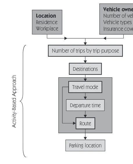
Figure 16.1 Dimensions of urban travel demand.

16.2

T

RAVEL AND

T

RAVEL

-R

ELATED

C

HOICES

Travel demand is determined by a number of interdependent decisions. Fig-ure 16.1 presents a list of travel or travel-related choices in approximate order from long run to short run. At the top are location and vehicle ownership decisions, and at the bottom is choice of parking location – which is often made on the spur of the moment while cruising for a free parking spot. The three choices to be considered in the two road-pricing studies, travel mode, departure time, and route, are typically intermediate in their time frame. The scheme in Figure 16.1 is not set in stone. Other decisions can be added, such as whether to purchase a transit pass, whether to chain trips, driving speed, and so on. And the time frame for decisions varies by type of trip and person. For example, the parking location decision of a commuter with employer-provided free parking is effectively deter-mined when the job is taken.

with today’s computing power it is infeasible to model every choice combination even for one person – let alone everyone in an urban area.

It would simplify matters greatly if travel decisions could be modeled as if they were made sequentially, rather than simultaneously. However, for a sequential approach to be valid the choices must be linked consistently in both “forward” and “backward” directions; that is, from top to bottom and from bottom to top in Figure 16.1. Consistency in the forward direction matters because choices made at one level impose constraints on lower levels. For example, a man who decides not to own a car cannot take a trip by driving alone unless he borrows or rents (or steals) one. And a woman who opts for the bus is constrained in her choice of departure time and route by the timetables and routes of bus lines in service. Consistency in the backward direction also matters because choices made at one level should affect the utility of choices made at earlier levels. Choice of route, for example, may affect travel time and therefore the attractiveness of driving rather than taking another mode.

There are several modeling approaches for studying travel demand that differ with respect to their inclusiveness of choice dimensions and their forward and backward consistency. Urban transportation planners have traditionally used the so-called classical (four-step) model, which incorporates the four choice boxes with heavy borders in Figure 16.1. The classical model has been applied with some success to analyze major infrastructure investments. But it is not well suited for evaluating policies such as road pricing that are designed to modify travel behavior in a substantial and/or comprehensive way. For one, the classical model excludes the other choice boxes in Figure 16.1. More fundamentally, the classical model lacks backward consistency because it does not incorporate complete or adequate feedback between the choice levels.

The Activity-Based Approach (ABA) provides another methodology for travel-demand analysis. The ABA seeks to derive travel behavior from the underlying demand to engage in work, shopping, recreation, and other activities. It incorpor-ates feedback between choice dimensions and, as indicated on the left-hand side of Figure 16.1, it encompasses the full range of short- and medium-run travel choices. However, despite rapid progress in recent years, a general ABA theory has yet to be developed, and applications continue to face difficulties with lim-ited data availability.

Discrete-choice models offer a third approach for studying travel demand. They have been applied in numerous travel-demand studies, including the two studies reviewed here. And forward consistency and backward consistency are intrinsic to the structure of discrete-choice models, as the review in the following section points out.

16.3

D

ISCRETE

-C

HOICE

M

ODELS OF

T

RAVEL

D

EMAND

16.3.1

The model specification

predict what choices an individual will make from a discrete set of alternatives such as combinations of destination, travel mode, departure time, and so on. Because of differences in their preferences, individuals who are faced with the same set of alternatives may make different choices. Each individual is assumed to know his or her utility from each alternative, and to select the one with the highest utility. But the analyst/econometrician does not know the individual’s utilities with certainty because of four potential sources of randomness:

• Unobserved attributes of the alternatives; for example, cleanliness of buses or the attractiveness of a shopping center.

• Unobserved socioeconomic or psychological factors; for example, family-related trip-scheduling constraints.

• Errors in measurement of alternative attributes (e.g., travel time) or socio-economic characteristics (e.g., income).

• The use of instrumental or proxy variables in lieu of the attributes of direct interest; for example, family size as a proxy for availability of a car to commute.

To reflect these uncertainties, and to insure that the theory is consistent with the econometrics, utility is modeled as a random variable. Formally, the utility from alternative i is written as follows:

Ui = Vi + εi. (16.1)

Term Vi in equation (16.1) is the deterministic part of the utility. It is a function of observable variables and taste parameters, and is referred to as measured utility

or systematic utility. Term εi is a random term that measures the influence of

unobservable individual-specific factors on utility. The model in equation (16.1) is referred to as a Linear Random Utility Model (LRUM), because εi enters the utility additively. The simplest case with a binary choice will be considered first, followed by the multinomial case with three or more alternatives.

16.3.2

The binary choice model

Suppose that there are two alternatives, 0 and 1. The probability that an indi-vidual selects alternative 1 is equal to the probability that U1 is larger than U0:

P1 = Pr(V1 + ε1 >V0 + ε0) = Pr(ε0 − ε1 < V1 − V0) =

Pr ε ε ,

µ µ

0 − 1 _< 1 − 0 ⎛

⎝⎜

⎞ ⎠⎟

V V

(16.2)

where µ (µ > 0) is a scale parameter with a value chosen so that (ε0 − ε1)/µ has a standard (normalized) probability distribution. If F(⋅) is the cumulative

The choice probabilities depend a priori on the probability distribution as-sumed for ε0 and ε1. The two most common choices are the Gumbel (also called double exponential) distribution and the normal distribution, which lead to the logit and probit models, respectively. While the two distributions have very similar shapes, only the logit model yields closed-form expressions for choice probabilities. Since logit models are featured in the two road-pricing studies, only the Gumbel distribution is considered henceforth.

The Gumbel distribution has a cumulative distribution function F(ε) = exp[−e−ε]. If ε0 and ε1 are identically and independently distributed (i.i.d.) Gumbel variables, then their difference, ε0 − ε1, has a logistic distribution and the probability of choosing alternative 1 in equation (16.2) is given by the binary logit formula:

0.5 if ∆V = 0. If µ is small, the model is nearly deterministic, and the choice

probabilities are close to zero or one when ∆V differs much from zero. But if µis large, P1 remains close to 0.5 even for large absolute values of ∆V. This means that the model is limited in its ability to forecast travelers’ choices. When there are many travelers in a sample who have the same values of ∆V, then P1 can be interpreted as the proportion of these travelers who choose alternative 1.

16.3.3

The multinomial model

In a multinomial model the number of alternatives in the universal choice set, A, exceeds two. The probability that alternative i ∈ A is chosen, Pi, is given by the

If the error terms for all alternatives are i.i.d. Gumbel distributed, the multinomial

logit (MNL) model results, and the choice probabilities are given by a generalized

For evaluating the welfare impact of a change in the travel environment such as a new toll, a measure of consumer’s or traveler’s surplus is required. A measure of surplus is also needed to extend the MNL model to the nested logit model considered below. Traveler’s surplus is defined to be the expected value of the maximum utility and, similar to conventional consumer’s surplus, it corresponds to the area under the demand curve. For the MNL model, traveler’s surplus is given (up to an additive constant) by the expression

CS E Uj V

j A

j j A

max= ⎛ ln exp .

⎝⎜

⎞ ⎠⎟ =

⎛ ⎝⎜

⎞ ⎠⎟

∈

∑

∈

µ

µ (16.6)

This term is variously called the logsum, inclusive value, or accessibility. Surplus is an increasing function of the systematic utility of each alternative, with a derivat-ive ∂CS/∂Vi = Pi, i ∈ A equal to the corresponding choice probability. Note that in a degenerate choice situation where 0 is the only alternative, equation (16.6) reduces to CS = V0.

T

HE

I

NDEPENDENCE OF

I

RRELEVANT

A

LTERNATIVES

(IIA)

PROPERTY The

closed-form expression for the MNL choice probabilities in equation (16.5) helps to reduce computation time for econometric estimation. But the MNL model has a property known as Independence of Irrelevant Alternatives (IIA) that is unrealistic in certain choice contexts. The IIA property can be stated in two equivalent ways (Ben-Akiva & Bierlaire 1999, p. 11): (i) “The ratio of the probabilities of any two alternatives is independent of the choice set,” or (ii) “The ratio of the choice probabilities of any two alternatives is unaffected by the systematic utilities of any other alternatives.”

To illustrate IIA, assume that a trip can be made either by auto or bus. If the two modes are equally attractive in terms of systematic utility, then V0 = V1 ≡ V, and by equation (16.3) each mode is chosen with probability 1/2. Suppose that the bus company now paints half of its buses red, and leaves the other half blue. Unless travelers care about color, red buses and blue buses will provide the same utility. But if the two types are treated as separate modes, there are now three alternatives and by equation (16.5) each will be chosen with probability 1/3. According to the MNL model, merely repainting the buses has increased bus ridership from 1/2 to 2/3. Furthermore, the ratio of the choice probabilities for auto and blue buses is unchanged (at unity) by introduction of the new red buses. And according to equation (16.6), surplus increases from V + µln(2) to

V + µ ln(3), which erroneously suggests that painting buses with different colors

is beneficial to travelers.

These implications of the MNL model are clearly unrealistic. One would expect patronage of the red buses to come (almost) exclusively at the expense of blue buses, so that the aggregate bus share of trips remains about 1/2, while the ratio of auto to blue bus travel rises to about 2.

Public transport alternative 1

Public transport alternative 1 Public transport

alternative 2

Public transport alternative 2 Auto

Public transport

(a) (b)

Auto

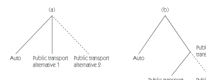
Figure 16.2 Decision trees for the (a) multinomial and (b) nested choice models.

single multinomial choice level, as shown in panel (a) of Figure 16.2, the choice can be decomposed into two nested stages, as shown in panel (b). In the first or outer stage, the traveler chooses between auto and public transport. If public transport is selected in the first stage, then a choice between public transport alternatives is made in the second or inner stage. If the two alternatives are essentially identical, as they are for red buses and blue buses, then the traveler effectively faces a binary choice between auto and homogeneous public trans-port, and the nested choice model collapses to the multinomial model with two alternatives. And if the two public transport modes are as dissimilar from each other as they are dissimilar from the auto, then the nested model again simplifies to the multinomial model, but now with three alternatives rather than two.

In most circumstances, public transport alternatives will be differentiated, but they will not be as distinct as public transport is from auto. If alternative 1 is bus, and alternative 2 is introduced as a new light rail system, rail can be expected to draw proportionally more travelers from buses so that the modal share of buses will fall by a larger percentage than the share for auto. This is consistent with the experience of US urban light rail systems, as mentioned in the Introduction. It should be noted that the IIA property does not hold in the aggregate if indi-viduals have different systematic utilities, because their choice probabilities differ. However, the IIA property is still restrictive, and this motivates consideration of the nested logit model.

T

HE NESTED LOGIT MODEL The nested logit model is obtained by nesting the

choices of a MNL model as just described. Let the universal choice set A be partitioned into M subsets or nests, Am, where Um=1,…,MAm = A. The individual first selects one of the nests, and then chooses an alternative from it. An example with

specific to the nest (ηm). For an alternative i in nest m, utility can be written as a variant of equation (16.1):

Ui = Vi + ηm + εi, i ∈ Am. (16.7) Error terms (εi) for alternatives within nest m are assumed to be i.i.d. Gumbel dis-tributed with scale parameter µm (which may depend on m). The conditional choice of alternative i ∈ Am is therefore described by a MNL model (see equation (16.5) ):

According to equation (16.6), the (random) surplus from choosing the best alternative from subset Am is µm ln ∑j∈Amexp[ (Vj + ηm)/µm] = CSm + ηm with CSm = µm ln ∑j∈Amexp(Vj/µm). At the outer choice level, the nest-specific error terms (ηm) are assumed to be i.i.d. Gumbel distributed with a common scale parameter µ. The probability of choosing subset Am is therefore as follows:

Finally, the unconditional probability of choosing alternative i ∈ Am is

Pi = Pm•Pi|Am. (16.10)

It can be shown that the correlation coefficient for the utilities of two alternatives,

i and j, within nest m is Corr(Ui,Uj) = 1 − µm

2_/µ2_{. Since the correlation coefficient is} assumed to be nonnegative, and by definition cannot exceed unity, it follows that µm/µ∈ [0,1]. If the estimated value of µm/µ lies outside this interval, it is evidence that the nested logit model is mis-specified. In the limiting case where µm = µ, m = 1, . . . , M, the nested logit model reduces to the MNL model.

T

HE MIXED LOGIT MODEL In the LRUM specification of equation (16.1) it is

The unconditional choice probabilities are obtained by integrating over the distri-bution of γ, and equation (16.5) is replaced by the mixed logit probability:

Pi =

冮

Γ

Pi(γ)g(γ)dγ, i ∈ A. (16.11)

The mixed logit model is very flexible in the sense that any random utility model can be approximated by it. The main drawback of the model relative to the logit model is that because more parameters are included, a larger sample size is required to obtain accurate parameter estimates.

16.3.4

Summary

Discrete-choice models have several merits for studying travel demand (Small & Winston 1999). They are firmly grounded in individual utility-maximizing behavior. The models are flexible in terms of inclusion of explanatory variables, functional form, and the degree of individual heterogeneity that is considered. Because individual rather than average values are used, better use can be made of information, and when large samples or panels of individuals are available the number of independent observations is also large. Discrete-choice models allow precise estimation of demand functions, and consequently also the benefits from transport improvements. And the models can be run “off the shelf,” using a number of user-friendly software packages.

A final advantage is that discrete-choice models provide an integrated and consistent treatment of choice situations with multiple dimensions. To see this, reconsider panel (b) of Figure 16.2 and note that the choices at the lower level, labeled public transport alternatives 1 and 2, could correspond to different departure times or different routes as per the general schema in Figure 16.1. The (prospective) utilities derived from choices made at each branch of the lower level are accounted for through the inclusive values. And the probability of each combined choice is specified by an expression of the form given in equa-tion (16.10). Choices that in practice may be made simultaneously by individuals are thus treated as if they were sequential – thereby circumventing the difficulty of dealing with large numbers of choice combinations.

16.4

S

TUDIES OF

B

EHAVIORAL

R

ESPONSES TO

R

OAD

P

RICING

the USA. Lam and Small employ data from an existing toll road, whereas Bhat and Castelar consider a hypothetical application of congestion pricing. Both studies examine behavioral responses to tolls, although the settings are quite different. Lam and Small’s analysis is described in some detail to demonstrate the import-ance of model specification and the ways in which travel-demand preference parameters can be estimated.

16.4.1

Time-of day congestion pricing

in Orange County, California

As noted in the Introduction, State Route 91 (SR91) was the first Value Pricing project. In 1995, two toll lanes were added to the median separating the five general-purpose free lanes that run in each direction. Tolls vary by time of day in each direction, and vehicles with three or more occupants (HOV3+) are charged half the published toll during certain congested hours and nothing the rest of the time. To study drivers’ propensity to use the toll lanes, Lam and Small (2001) obtained data for about 400 individuals from a 1998 mail survey and a one-week trip diary. Travel times on the toll lanes and free lanes were calculated with loop-detector data. These data were used to estimate discrete-choice models of travel mode,departure time, and route.Route choice is a choice between the toll lanes and the free lanes, which Lam and Small refer to as a choice of lane. Travel mode, departure time, and lane choices can be estimated individually or jointly. Joint estimation is preferable because of potential endogeneity bias from individual choice estimation if related choices are treated as fixed. (An example of endogeneity bias is given below.) But following Lam and Small, it is instructive to consider both estimation procedures in order to examine the robustness of the estimates. Attention is focused here on their model of choice of lane, and their model of joint choice of departure time and lane.

C

HOICE OF LANE ALONE In the lane-choice model, both travel mode and

departure time are treated as fixed, and travel time and cost are assumed to be exogenous. Drivers therefore face a binary choice between the free lanes (i = 0)

and the toll lanes (i = 1). A binary logit model is used for estimation. The main

explanatory variables are expected travel time (t), variability of travel time (r), and travel cost (c). Since individuals typically dislike each of these attributes, the estimated coefficients on each are expected to be negative. The measured values of t, r, and c vary by time of day. The loop-detector data show that free-flow conditions prevail on the toll lanes almost all the time. Travel time on the free lanes has a larger expected value and a larger variability.

Since the values of the choice attributes, and possibly also the behavioral parameters, differ across individuals, individuals will now be distinguished by an index n. The utility of choice i for individual n, given generically by equation (16.1), is written

where xn is a vector of individual socioeconomic characteristics such as age and income. The explanatory variables, tin, rin, and cin, i = 0,1, are evaluated at the time when individual n travels. Expected travel time, tin, is measured by the median travel time on lane i, and travel time variability, rin, by the difference between the 90th and the 50th percentiles of the travel time. (These two measures provided a better fit than did the mean and standard deviation.)

The third explanatory variable, cin, is the toll cost on lane i. Whereas tin and rin are the same for all individuals who use lane i in the same 30-minute time period, cin depends on n through vehicle occupancy in two ways: first, because the toll cost is assumed to be shared evenly between occupants; and, second, because vehicles with three or more occupants pay either half the published toll or nothing. The simplest version of equation (16.12) to be estimated is linear in the attributes:

Uin = γin0 + γnttin + γnrrin + γnccin + εin, i = 0,1. (16.13) Because the free lanes and toll lanes are on the same highway, the attributes tin,

rin, and cin are assumed to be valued equally, so that the corresponding coefficients γnt, γnr and γnc do not depend on i. (In other choice situations, the coefficients could differ; for example, the disutility of travel time may be less on scenic routes.) However, the coefficients are allowed to vary by individual. For purpose of normalization, the constant term for the free lanes, γ0n0, is set to 0, and the scale parameter of the MNL is set to unity (µ = 1). The difference between the system-atic utilities of the toll lanes and free lanes, ∆V = V1n − V0n in equation (16.3), is therefore

∆V = γ1n0 + γnt(t1n − t0n) + γnr(r1n − r0n) + γncc1n. (16.14) The relative disutility from travel time is referred to in the transportation litera-ture as the Value of Time (VOT). Formally, the VOT is defined to be the marginal rate of substitution between travel time and money. From equation (16.13), this is given by

By analogy with the VOT, the Value of Reliability (VOR) is defined to be the marginal rate of substitution between travel time variability and money:

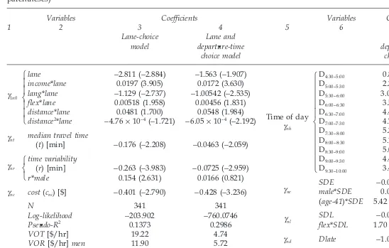
Column 3 of Table 16.1 presents the estimation results for the best-fitting variant of the lane-choice model. The dependent variable is the choice of lane. All vari-ables are measured in minutes and dollars except for income, which is measured in thousands of dollars. In the lower half of Table 16.1, N denotes the sample size. The log-likelihood statistic in the next row is the maximum value of the likelihood function achieved in the maximum likelihood estimation procedure; it can be used to compare similar models in terms of goodness-of-fit. (Note that the models corresponding to columns 3 and 4 are not similar, since the second one includes additional variables that appear in column 6.) Finally, the Pseudo-R2 statistic is given by 1 −ᏸ_/ᏸ0_{, where ᏸ is the log-likelihood of the model, and ᏸ}0 is the log-likelihood of a restricted model that includes only constant terms. Since ᏸ0 _{≤ ᏸ ≤ 0, the Pseudo-R}2 _{lies in the interval [0,1].}

Estimates for the three main explanatory variables are reported in the middle rows of Table 16.1. The standard errors of the estimates can be obtained from the point estimates and the asymptotic t-statistics (in parentheses). For example, the standard error for the lane dummy, γ1n0, is −2.811/−2.884 = 0.9747. The coeffi-cients γnt and γnc are assumed to be independent of individual-specific character-istics. Both have the expected negative sign. Expressed in terms of equation (16.14), the probability of choosing the toll lanes is a decreasing function of the difference between the toll and free lanes in expected travel time and also a decreasing function of the toll. Using equation (16.15), the point estimate of VOT is as follows:

(The factor of 1.37 is added to correct for missing loop-detector data; see Lam and Small (2001, p. 234).)

To allow for differences between the sexes in the cost of travel-time variability, an interaction term is included between r and a dummy variable male, set equal to 1 for males and 0 for females. The coefficient on this variable is positive, which indicates that men are less sensitive to travel-time variability. Indeed, the estimated coefficient for men of −0.263 + 0.154 = −0.109 is less than half in magnitude the estimated value of −0.263 for women. The point estimates of VOR for men and women are derived in the same way as for VOT. Given the assumption of equal VOT, the risk aversion estimates (0.62 and 1.49) are correspondingly much higher for women. This finding – which is supported by other recent research – may be due to the tighter time constraints that women face as they juggle work demands with a lion’s share of family responsibilities.

274

Lane-choice Lane and Lane and

model departure-time departure-time

choice model choice model

γ1n0

lane −2.811 (−2.884) −1.563 (−1.907)

income*lane 0.0197 (3.905) 0.0172 (3.630)

lang*lane −1.129 (−2.737) −1.00542 (−2.535)

flex*lane 0.00518 (1.958) 0.00456 (1.831)

distance*lane 0.0481 (1.700) 0.0548 (1.984)

distance2_{*lane −4.76 × 10}−4 _{(−1.721) −6.05 × 10}−4 _(−2.192)

γnt median travel time

(t) [min] −0.176 (−2.208) −0.0463 (−2.059)

γnr

time variability

(r) [min] −0.263 (−3.983) −0.0725 (−2.959)

r*male 0.154 (2.631) 0.0166 (0.821)

γnc cost (cni) [$] −0.401 (−2.790) −0.428 (−3.236)

Source: Lam and Small (2001), tables 5 (Model 1g) and 8 (Model 2d)

⎧

male*SDE 0.0126 (2.633) (age-41)*SDE 5.42 × 10−4 _(2.345)

γnl SDL

−0.0465 (−3.988)

flex*SDL 1.70 × 10−4 _(1.965)

γnd Dlate −1.0784 (−2.341)

interval). A possible explanation for the counter-intuitive positive effect of flexibil-ity is that people with flexible hours may have more opportunflexibil-ity than do workers with rigid hours to advance their careers by spending time at the office and/or being punctual when they have appointments. Finally, the variable distance, which refers to total trip distance in miles, is interacted quadratically with the lane dummy. The estimates indicate that up to a distance of about 50 miles (which covers about three-quarters of the sample), people who make longer trips favor the toll lanes, possibly because they face tighter daily time constraints than do people with short trips and therefore value more highly savings in time.

C

HOICEOFLANEANDDEPARTURETIME Departure time is treated as given in

the lane-choice model. This is a dubious specification because departure time affects all three of the explanatory variables: expected travel time, variability in travel time, and toll. Because there may be unobserved factors that influence both departure time choice and lane choice, the explanatory variables and the error terms in equation (16.13) may be correlated, which invalidates the binary logit model.

To correct for this type of endogeneity bias, lane choice and time-of-day choice must be modeled as a joint decision. Time-of-day choice was modeled as a choice between 12 half-hour arrival-time intervals from 4:00 to 10:00. Trip-timing prefer-ences were included by adding four terms to the systematic utility function:

• Constants for each arrival time interval.

• SDE: Schedule Delay Early, equal to Max[0,T], where T is the difference between official work time and the lower limit of the half-hour time interval. • SDL: Schedule Delay Late, equal to Max[0,−T].

• Dlate: A dummy variable equal to 1if T < 0, and 0 otherwise.

Variable SDE measures the extent to which individuals arrive at work earlier than desired. SDL is defined analogously for late arrival. Dlate is a discrete vari-able that captures any fixed costs of arriving late, such as disapproval from the employer. With the inclusion of these variables, the estimating equation becomes, in place of equation (16.13),

Uihn = γin0 + γnttihn + γnrrihn + γnccihn + γnhDh + γneSDEihn

+ γnlSDLihn + γndDlateihn + εihn, (16.18)

where γnh is the coefficient for arrival time interval h, Dh is a dummy variable for work arrival during this interval, and index h indicates that variables now also depend on the time interval.

other roads as well, except for a 5-mile segment that was assumed to be con-gestion free.

With two decisions, lane and time of day, it is natural to consider a nested logit model for estimation. Since it is not obvious whether lane choice or time-of-day choice belongs at the upper branch of the decision tree, both specifications were tested. However, both produced estimates of the scale parameter ratio, µm/µ, outside the admissible [0,1] interval. Therefore, a MNL model was used instead.

The MNL estimates for variables that also appear in the lane-choice model are presented in column 4 of Table 16.1. Estimates for the lane constant and inter-action terms do not differ greatly from those of the lane-choice model, and the coefficient on cost, γnc, is also similar. However, the coefficients on expected travel time and variability, γnt and γnr, are much smaller. One possible reason is that the assumption about travel times outside SR91 is inaccurate. But an alternative specification in which outside travel times were ignored also yielded relatively low estimates for these parameters. This suggests that the differences in results are driven by severe endogeneity bias in the lane-choice model from treating departure time choice as given. Such a bias could be tested formally using a Hausman specification test. The large differences between the coefficient estimates in the two models would undoubtedly lead to rejection of the null hypothesis that departure times are exogenous. (Lam and Small also estimated MNL and nested logit models for joint lane and mode choice decisions. The estimates for VOT and VOR were broadly similar to those for the lane-choice model, which indicates that any endogeneity bias from disregarding mode choice is less severe.) The estimates for VOT and VOR will be biased upward if there are unobserved factors that incline people to choose the toll lanes at peak times, because median travel time and variability are higher during the peak. For example, an indi-vidual with a job that starts at a popular time and requires punctuality will prefer to travel at the height of the rush hour and to use the toll lanes to reduce the chance of delay. If so, the unobserved factor, type of job, induces a positive correlation between departure time at the peak and use of the toll lanes. In any case, the relatively low estimated coefficients in the joint model for expected travel time and variability translate to low values for VOT and VOR as reported at the bottom of column 4. The risk aversion coefficient remains larger for women than for men, although this difference is no longer statistically significant.

Column 7 of Table 16.1 reports estimates for variables related to departure-time choice. The reference alternative for departure-time of day is the earliest departure-time interval, 4:00–4:30. Time-of-day coefficients, γnh, for the remaining 11 time intervals exhibit a hump-shaped pattern, with a maximum at 7:30–8:00. Predictably enough, this implies an aversion to traveling either very early or very late in the morning. All three schedule-delay cost coefficients are negative as expected. The positive interaction term coefficients for SDE indicate that males and older workers are less averse to arriving early – perhaps because they have fewer family obligations. Using the coefficient estimates, it is possible to compute various marginal rates of substitution. For example, to avoid arriving late an individual would be willing to pay a price of γnd/γnc= (−1.0784)/(−0.428) = $2.52. In order to avoid

arriving a minute earlier, a 31-year-old female would be willing to incur an extra travel time of [−0.0285 + (31 − 41) × (5.42 × 10−4_{)]/(−0.0463) = 0.73 minutes. These} estimates are representative of those obtained from various trip-timing studies over the past 20 years.

16.4.2

Congestion pricing in the San Francisco Bay Area

For their study of SR91, Lam and Small (2001) were able to use Revealed Preference

(RP) data; that is, data on travel choices that people actually made. But sufficient RP data are sometimes lacking. This was the case for Bhat and Castelar’s (2002) study of congestion pricing in the San Francisco Bay Area. Several congestion-pricing schemes have been proposed for the Bay Area over the past 30 years, but none have been implemented. And although the Golden Gate and several other bridges are tolled, the tolls are constant throughout the day. RP data on responses to time-of-day toll differentials were therefore not available.

To overcome this deficiency, Bhat and Castelar drew on a survey of people who reported crossing one of the Bay Bridges at least once a week during the morning peak. Those surveyed were asked to make choices from a set of hypo-thetical alternatives, discussed below. Their responses comprise what is called

Stated Preference (SP) data. Bhat and Castelar combined this SP data with RP data

from the 1996 San Francisco Bay Area Travel Study.

To accommodate unobserved heterogeneity in individual preferences, Bhat and Castelar adopt a mixed MNL model (see equation (16.11)). This model also allows them to test for behavior known as state dependence. State dependence occurs in a combined RP/SP context when a respondent’s revealed choice influ-ences his or her stated choices. Habit persistence or risk aversion will tend to create positive state dependence, whereas variety-seeking or frustration with the alternative currently chosen will induce negative state dependence. Both the sign and the intensity of the state-dependence effect can vary across individuals, and the mixed MNL model can accommodate this type of heterogeneity.

The SP data used in Bhat and Castelar’s study were generated for each survey respondent by taking his or her reported trip as a reference, and developing SP scenarios that involve alternative combinations of mode and time of day. The modes include driving alone, carpooling, and two forms of public transportation. Peak and off-peak periods were also defined for the drive-alone auto mode, giving a total of five alternatives. Two congestion-pricing scenarios were con-structed by assuming a $2 or $4 increase in the cost of the “drive alone – peak” alternative (an increase of 44 percent or 87 percent in mean travel cost). Discussion is limited here to the $4 scenario and to the two most diverse model specifica-tions considered: an MNL model that uses cross-sectional data, and a general model that uses panel data and includes both unobserved heterogeneity and state-dependence effects. The results are reported in Table 16.2.

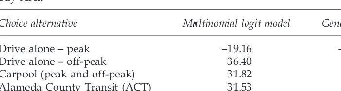
Table 16.2 Simulated percentage changes in alternative choice shares in response to a $4 increase in the “drive alone – peak” travel cost, San Francisco Bay Area

Choice alternative Multinomial logit model General model

Drive alone – peak −19.16 −18.44

Drive alone – off-peak 36.40 26.39

Carpool (peak and off-peak) 31.82 39.98

Alameda County Transit (ACT) 31.53 36.91

Bay Area Rapid Transit (BART) 28.65 28.66

Source: Bhat and Castelar (2002), table 6

property, the MNL model predicts similar percentage increases in shares of the other alternatives. (The increases are not identical because the sample of indi-viduals is heterogeneous and, as noted in Section 16.3, aggregate MNL choice shares do not obey IIA.) The general model predicts a substantially smaller per-centage increase in driving alone off-peak, and a substantially larger perper-centage increase in carpooling. In terms of congestion relief, the MNL therefore slightly overpredicts the benefits that would accrue from reduced peak driving by solo drivers, but underpredicts the potential increase in congestion from more carpooling during the peak.

Bhat and Castelar also report estimates of VOT, which they assume to be homogeneous in the population. When the RP data are used, their MNL model yields an estimate of about $20 per hour. But when the SP data are used either alone or in combination with the RP data, the estimated VOT falls to about $11 per hour. Though not as drastic as the differences in estimated VOT in Table 16.1, the discrepancy is still appreciable. In part, it may be due to lack of adequate variation of monetary costs and travel times in the RP data. One advantage of using SP data is that the degree of variation can be controlled through the design of the hypothetical alternatives. The discrepancy is also consistent with a well-documented tendency of SP survey respondents to overstate their propensity to change behavior. This would mean that changes in travel time induced by the $4 charge would be inflated, with corresponding reductions in the implied VOT.

16.5

C

ONCLUSION

is evident in Lam and Small’s study of SR91 from the fact that their combined lane and departure-time choice model yields very different estimates of VOT and VOR than does their lane-choice model.

A second lesson is that model specification can influence results materially. For instance, Bhat and Castelar’s general model predicts different responses to a toll than does their more restrictive multinomial logit model, which suffers from the Independence of Irrelevant Alternatives property. It is also important to include the appropriate explanatory variables in the regression equations. For example, several road-pricing studies have found that motorists dislike travel time under congested conditions much more than under free-flow conditions, and it is there-fore crucial to distinguish the two variables when predicting travel behavior.

A third lesson is that people differ widely in their travel behavior. Some are wedded to their cars and have rigid daily schedules, while others are more adaptable and will shift mode, travel time, or route in response to tolls. Opportun-ities to save travel time are the main attraction of using toll roads, and estimates of the value that people place on time savings and enhanced reliability vary with income, sex, trip purpose, and other socioeconomic characteristics. Not surpris-ingly, high-income individuals are more inclined to use toll lanes, and this might suggest that road pricing favors the rich. However, studies of SR91 and other toll-lanes projects show that usage is actually quite varied. Few people take the toll lanes consistently, and even lower-income people use them occasionally when they are especially pressed for time.

The benefits and welfare-distributional effects from road pricing naturally depend on the design of the scheme and the setting. There is a big difference between the toll-lanes projects that have been introduced in the USA and the much larger area-based systems in place or planned for Europe. One should not expect the findings derived from a facility such as SR91 – which has toll-free lanes running in parallel with the toll lanes – to be transferable to a much larger and more complex scheme such as in London, where payment is difficult to avoid.

In the long run, the impacts of road pricing will extend beyond the relatively short-term choice dimensions considered in the two studies reviewed here to encompass other dimensions of behavior shown in Figure 16.1, such as resid-ential and workplace locations and vehicle ownership. Both the practice of road pricing and an understanding of its impacts are developing rapidly, and many of the details in this essay will soon be obsolete. Nevertheless, it is hoped that readers, with the advantage of hindsight, can still benefit from the relat-ively early perspective on road pricing and urban passenger travel demand offered here.

Acknowledgments

Bibliography

Travel demand

Bates, J. 2000: History of demand modeling. In D. A. Hensher and K. J. Button (eds.),

Handbook of Transport Modelling, vol. 1. Oxford: Elsevier Science, 11–33.

Small, K. A. and Winston, C. 1999: The demand for transportation: models and applica-tions. In J. A. Gómez-Ibáñez, W. B. Tye, and C. Winston (eds.), Essays in Transportation Economics and Policy: A Handbook in Honor of John R. Meyer. Washington, DC: Brookings Institution Press, 11–55.

Discrete-choice models

Ben-Akiva, M. and Bierlaire, M. 1999: Discrete choice methods and their applications to short term travel decisions. In R. W. Hall (ed.), Handbook of Transportation Science. Boston: Kluwer, 5–33.

Studies of road pricing

Bhat, C. R. and Castelar, S. 2002: A unified mixed logit framework for modelling revealed and stated preferences: formulation and application to congestion pricing in the San Francisco Bay area. Transportation Research B, 36B, 593–616.

Brownstone, D., Ghosh, A., Golob, T. F., Kazimi, C., and Van Amelsfort, D. 2003: Drivers’ willingness-to pay to reduce travel time: evidence from the San Diego I-15 congestion pricing project. Transportation Research A, 37A, 373–87.

Burris, M. W. and Pendyala, R. M. 2002: Discrete choice models of traveler participation in differential time of day pricing programs. Transport Policy, 9, 241–51.

Erhardt, G. D., Koppelman, F. S., Freedman, J., Davidson, W. A., and Mullins, A. 2003: Modeling the choice to use toll and high-occupancy vehicle facilities. Transportation Research Record 1854, 135–43.