Multiple Linear Regression Using Rank-Based Test of Asymptotic Free Distribution

(1)

Distribution

Kuntoro†

†Department of Biostatistics and Population Study, Airlangga University School of Public Health, Surabaya 60115, Indonesia

(e-mail: kuntoro1@indo.net.id)

Abstract

An experimental design is a classical approach for proving causal relationship. Some-time a study in the field of public health including maternal child health study is difficult to control experimental conditions properly beside an ethical reason for doing an exper-iment. A multiple regression approach that involves a dependent variable and a number of independent variables in its model could be an alternative solution for proving causal relationship in a non experimental study.

In maternal child health study that involves variables in ordinal scales such knowledge, attitude and practice, an ordinary regression model is not the best choice for analyzing those variables. A rank-based test of asymptotic free distribution is the better alternative solution than that one. The Jaeckel - Hettmansperger- McKean, HM is used to demon-strate the effect of knowledge about safe water and attitude upon drinking unboiled water on practice of drinking unboiled water. The data obtained from sample of mothers having under five yrears children in 14 districts in East Java Province, Indonesia.

The results show that Hodges - Lehmann estimate of tau is 0.5329. The Jaeckal distribution measure is 0.00002721. The HM statistic for testing the null hypothesis, Beta1 = Beta2 = 0 is 0.000102. Under null hypothesis, HM statistic has a sampling distribution that approximates to Chi Square distribution. Since the result is less than critical point of 5.99 (degree of freedom = 2 and level of significance of 0.05), the alternative hypothesis fails to be rejected. That means there are no effect of konwledge and attitude on practice. It is concluded that the procedure is quite simple compared to ordinary regression procedure, no assumption is made. It is easy to use. It is recommended to use HM statistic in analyizing data obtainded from public health study as well as social study.

Keywords: non experimental study ordinal scale HM statistic

1 Introduction

(2)

independent variable and Y variable as dependent variable. A regression model as a statistical tool looks like an experimental model as a research methodology tool in which they connect between the independent variable and the dependent variable (Joreskorg and Sorgom, 1988).

Today many researchers from the areas of social sciences and economics as well as the behavioral sciences implement the regression model to demonstrate causal relationship in the nonexperimental conditions. They use the quantitative approach for collecting the data. Most data have an ordinal scale such as motivation, attitude, knowledge, practice, performance. Hence, one of the classical assumptions of ordinary regression model related to the scale of the data is violated.

Researchers who are not statisticians argue that a statistical method is just a tool for support their findings no matter it violates or it does not violates the assumptions. They considers that a statistical tool is not an objective of the research process. A statistician should explain to them that the results of the research are valuable optimally when they are analyzed by mean of an appropriate statistical method. Over years statisticians have developed statistical methods that are expected to support the researchers in analyzing their data properly. This paper discusses the application of regression model when the data do not have an interval or a ratio scale. The first section discusses basic concept of nonparametric multiple linear regression. The second one implements that statistical method in the data collected from health research.

2 Basic Concept

The basic concept to be discussed includes the data to be used, the asumption of the multiple regression model, the hypothesis to be formulated, the procedure for computing the statistic, and in the case where ties exist.

2.1 Data

Suppose, x′ ₌ _⌊x

1x2 . . . xp⌋ is a row vector of p independent variables, and x′1 =

(x11, x21, . . . , xp1), . . . , x′n = (x1n, x2n, . . . , xpn) are n fixed values of this vector. ¿From each vector x′_1, _x′_{2, . . . ,} _x′

n the value of the single response random dependent variable Y is observed. Hence, a set of observationsY1, Y2, . . . , Yn is obtained, in which

Yi is the value of the dependent variable whenx′=x′i.

2.2 Assumptions

First of all, the following equation represents the multiple regression model:

Yi=ξ+β1x1i+β2x2i+. . .+βpxpi+ǫi=ξ+x ′

iβ (1)

where i = 1, 2, . . . , n; x′

1 = (x11, x21, . . . , xp1), . . . , x′n = (x1n, x2n, . . . , xpn) are known constant vectors; is the unknown intercept parameter, and β′ _{= [}_β

1β2 . . . βp] is

a row vector of unknown parameters that is usually referred to as the set of regression coefficients. To make simple understanding, equation 1 can be written in matrix notation.

Suppose

Moreover, equation 1 can be expressed in matrix notation as follows.

(3)

Secondly, the error random variables ǫ1, ǫ2, . . . , ǫn are a random sample from a continuous distribution which is symmetric about its Median 0. It has cumulative dis-tribution function F(·) and has probability density function f(·) that satisfies the mild condition thatR+∞

−∞ f

2₍_t₎_{dt <}_∞_.

2.3 Hypothesis

In this regression model, it is emphasized to test the null hypothesis that a specific subset βq of the regression parametersβ are equal to zero. Without loss of generality (because the ordering of (x1, β1),(x2, β2), . . . ,(xp, βp) pairs in the equation 1 is arbitrary), this subsetβq is taken to be the first q components ofβ, that is,β′

q = [β1β2 . . . βq] is taken. Hence, the hypothesis to be tested is

H0:

The statement mentioned above tells that the null hypothesis accepts that the inde-pendent variables x1, x2, . . . , xq do not have the significant roles in determining the value of the dependent variable Y. (In many setting, the interest is to assess the effect of all the independent variables simultaneously, which is appropriate to taking q = p in the null hypothesis (4).

2.4 Procedure

In order to compute theJaeckel - Hettmansperger - McKean, test statistic HM, it is processed in several steps clearly.

The first step is to obtain an unrestricted estimator for the vector of regression param-eters . SupposeRi(β) is the rank ofYi−x′iβamongY1−x′1β, Y2−x′2β, . . . , Yn−x′nβ as a function ofβ, for = 1, 2, . . . , n. The unrestricted estimator forβis appropriate to a special case of a class of estimator proposed by Jaeckel (1972). Hence, the estimator of the value of β, say, ˆβ minimizes the measure of dispersion:

DJ(Y −Xβ) = (12)

In general, the estimator ˆβdoes not have an expression of closed-form and methods of iterative computer is generally needed to obtain numerical solution. It can be accomplished by using command of ”RREG” in MINITAB program to obtain that value.

The second step is to involve repeating the steps in order to obtain ˆβ. Except that minimization of the measure of dispersion Jaeckel DJ(Y −Xβ) is obtained under the

condition that the null hypothesis is true, say, βq = 0, with βp₋q unspecified. Suppose ˆ

β0 represents the value of β which minimizes DJ(Y −Xβ) in equation (5) under the

null constraint that βq = 0. Once again, ˆβ0 will not be available in an expression of

closed-form. It will be used command of ”RREG” in MINITAB program to obtain its value.

SupposeDJ(Y −Xβˆ) andDJ(Y −Xβˆ0) respectively represent the overall minimum

and the minimum under the null constraint that βq = 0of the measure of dispersion of JaeckelDJ(Y −Xβ). Furthermore, it is set that:

D∗

J=DJ(Y −Xβˆ0)−DJ(Y −Xβˆ) (6)

whereD∗

Jis the reduction in dispersion of Jaeckel from fitting the full model as opposed to the reduced model which is appropriate to the null hypothesis (4) constraint thatβq = 0.

The third step is to compute a consistent estimator of the parameter:

τ= [12]−1

(4)

By combining the results of the three steps, theJaeckel - Hettmansperger - McK-ean test statistic HMis expressed by equation as follows:

HM = 2D ∗ J ˆ

τ (8)

If the null hypothesis (4) is true, and n tends to be infinite, HM statistic has an asymptotic chi square distribution (χ2_{) with q degree of freedom which is appropriate to}

the q constraints placed onβ under the null hypothesis. To test the null hypothesis,

H0:

£ β′

q= 0; β′p₋q= (βq+1βq+2; . . . βp) and ξ not specif ied

¤

against the alternative hypothesis,

H0:

£ β′

q= 0; β′p−q6= (βq+1βq+2; . . . βp) and ξ not specif ied

¤

by selecting the level of significance ofα,

Reject the null hypothesis if HM ≥χ2

q,α Accept the null hypothesis if HM < χ2

q,α

(9)

where χ2

q,α is the upperαpercentile point of chi square distribution with the q degree of freedom. The value ofχ2

q,α can be obtained from the statistical table which is available in the text-books of statististics.

Hettmansperger and McKean (1977) and McKean and Sheather (1991) remind that in application using small to moderate sample size, the chi square distribution is often too light-tailed. They suggest to replace the percentile of chi square χ2

q,α by:

qFq,n−p−1;α

where Fq,n−p−1;α is the upperαpercentile of theFdistribution with q numerator degree of freedom and n - p - 1 denominator degree of freedom.

TIES : when the ties exist amongY1−x′1β, Y2−x′2β, . . . , Yn−x′nβ, use the rank average to break the ties in computing the minimum ofDJ(Y −Xβ). Similarly when the

ties exist among Y1−x′1β0, Y2−x′2β0, . . . , Yn−x′nβ0, use the rank average to break

(5)

3 Material And Method

3.1 Material

(6)

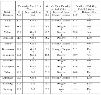
The following table shows the highest percentage of level of knowledge, attitude, and practice and their scores.

Table 1. The Highest Percentage of Level of Knowledge, Attitude, and Practice

Knowledge About Safe Water

Attitude Upon Drinking Unboiled Water

Practice of Drinking Unboiled Water

District % Level and Score % Level and Score % Kategori/Skor

Ponorogo 79.9 Bad 69.4 Strongly Disagree 64.9 Never

1 5 3

Blitar 80.0 Good 50.0 Strongly Disagree 64.5 Never

2 5 3

Kediri 81.3 Bad 46.1 Disagree 53.5 Never

1 4 3

Malang 65.6 Good 42.5 Disagree 59.0 Never

2 4 3

Lumajang 61.7 Good 48.2 Disagree 54.8 Ever

2 4 2

Jember 74.0 Good 53.4 Strongly Disagree 52.5 Never

2 5 3

Bondowoso 69.1 Good 49.7 Strongly Disagree 51.7 Ever

2 5 2

Probolinggo 65.3 Good 73.7 Disagree 50.7 Never

2 4 3

Mojokerto 74.1 Good 55.7 Disagree 58.6 Never

2 4 3

Bojonegoro 0.2 Good 48.6 Disagree 63.6 Never

2 4 3

Tuban 52.0 Bad 51.0 Disagree 63.3 Ever

1 4 2

Lamongan 64.0 Good 49.6 Strongly Disagree 58.8 Ever

2 5 2

Sampang 50.9 Bad 45.7 Disagree 49.1 Ever

1 4 2

Sumenep 68.6 Bad 37.9 Agree 42.4 Ever

(7)

3.2 Method

By applying Secondary Data Analysis Method (Nachmias, 1987) The scores of three variables are analyzed by mean of MINITAB program in order to compute HM statistic.

First of all : Enter the scores of variables of knowledge (knowl), attitude(attit), and practice (pract) to the spreadsheet of MINITAB as follows.

Row Knowl Attit Pract

Create matrices of M1, M2, and M3 that state the null hypothesis 1, the null hypothesis 2, and the null hypothesis 3 respectively.

The null hypothesis 1: H01[β1=β2= 0; ξ unspecif ied] MTB > COPY C4-C5 M1 MTB > PRINT M1 MTB > COPY C6-C7 M2 MTB > PRINT M2 MTB > COPY C8-C9 M3 MTB > PRINT M3

(8)

Matrix M3

0 1

MTB >

Then M3 =£

0 1 ¤

Third:

Operate the command of Rank Regression (RREG) to obtain the value that can be used to compute measure of dispersion Jaeckel,HM statistic and to obtain the equation of rank regression.

To test the null hypothesis 1:

MTB > RREG ’Pract’ 2 ’Attit’ ’Knowl’; SUBC> HYPOTHESIS M1.

4 Result And Discussion

4.1 To test the null hypothesis :

β

₁

=

_β

2

= 0

The statement of the null hypothesis is the independent variable of knowledge about safe water and the independent variable of attitude upon drinking unboiled water do not affect the dependent variable of practice of drinking unboiled water.

This is the ”print out ” of MINITAB :

The regression equation is

Pract = 2.50 + 0.000 Attit + 0.000 Knowl

Coefficient Coefficient Predictor Rank Least-sq Rank Least-sq Constant 2.4999 1.8038 0.9790 0.8132 Attit 0.0000 0.1044 0.2421 0.2011 Knowl 0.0000 0.1994 0.3904 0.3242

Hodges-Lehmann estimate of tau = 0.5329 Least-squares S = %2

ANOVA for hypothesis matrix M1

Dispersion

Reduced model Full model DF F Denom DF Approx F

Rank 5.54256258 5.54258979 2 0.3208 11 -0.00

Least-sq 3.42857143 3.12341772 2 0.2839 11 0.54

Unusual observations

Observation Attit Pract Pseudo Fit SE Fit Residual 14 2.00 2.000 2.261 2.500 0.522 -0.500 X

X denotes an observation whose X value gives it large influence.

Moreover, compute measure of dispersion Jaeckel as follows.

D∗

J =DJ(Y −Xβˆ0)−DJ(Y −Xβˆ) = 5,54258979−5,54256258 = 0,00002721 q=degreesof f reedom= 2, ˆτ= 0,5329

HM = 2D∗

J/τˆ= 2∗0,00002721/0,5329 = 0,000102

Furthermore, the result is compared to the critical point in Chi Square table. When we choose level of significance of α= 0,05 with 2 degree of freedom, the critical point is 5,99. Since HM statistic <5,99 then the null hypothesis that statesβ1=β2= 0 is to be

(9)

4.2 To test the null hypothesis :

β

₁

= 0

The statement of the null hypothesis is the independent variable of knowledge about safe water does not affect practice of drinking unboiled water.

This is the "print out " of MINITAB :

Pract = 2.50 + 0.000 Knowl + 0.000 Attit

Coefficient Coefficient Predictor Rank Least-sq Rank Least-sq Constant 2.4999 1.8038 0.9790 0.8132 Knowl 0.0000 0.1994 0.3904 0.3242 Attit 0.0000 0.1044 0.2421 0.2011

Dispersion

Rank 5.54256347 5.54258979 1 0.3208 11 -0.00

Least-sq 3.23076923 3.12341772 1 0.2839 11 0.38

Observation Knowl Pract Pseudo Fit SE Fit Residual 14 1.00 2.000 2.261 2.500 0.522 -0.500 X

MTB >

4.3 To test the null hypothesis :

β

₂

= 0

The statement of the null hypothesis is the independent variable of attitude upon drinking unboiled water does not affect practice of drinking unboiled water.

This is the ”print out ” of MINITAB :

The regression equation is

PRAKT = 2.50 + 0.000 Knowl + 0.000 Attit

Coefficient Coefficient Predictor Rank Least-sq Rank Least-sq Constant 2.4999 1.8038 0.9790 0.8132 Knowl 0.0000 0.1994 0.3904 0.3242 Attit 0.0000 0.1044 0.2421 0.2011

Dispersion

Rank 5.54256311 5.54258979 1 0.3208 11 -0.00

Least-sq 3.20000000 3.12341772 1 0.2839 11 0.27

Observation Knowl Pract Pseudo Fit SE Fit Residual 14 1.00 2.000 2.261 2.500 0.522 -0.500 X

MTB >

(10)

about safe water does not affect the dependent variable of practice of drinking unboiled water, and also the independent variable of attitude upon drinking unboiled water does not affect the dependent variable of practice of drinking unboiled water.

Like parametric multiple regression model, rank regression model also requires the assumption that there is no collinearity among independent variables. MINITAB will drop the independent variable which is highly correlated with other independent variable and there is no hypothesis to be tested. Before doing RR command in MINITAB, collinearity among independent variables can be detected by computing correlation coefficient for ordinal scale such as Spearman rank correlation coefficient.

5 Conclusion And Recommendation

It is concluded that knowledge about safe water and attitude upon drinking unboiled water simultaneously do not affect practice of drinking unboiled water. Each independent variable does not affect practice of drinking water.

The procedure is quite simple compared to ordinary regression procedure. The as-sumption made is no collinearity among independent variables. It is easy to use. It is recommended to use HM statistic in analyzing the data having ordinal scale obtained from public health study as well as social study.

References

[1] Campbell, D.T., and Stanley, J.C. (1966).Experimental and Quasi-Experimental Designs for Research.Rand McNally College Publishing Company. Chicago.

[2] Fowler, Jr., F.J. (1984). Survey Research Methods. Sage Publications.Beverly Hills.

[3] Hollander, M., and Wolfe, D.A. (1999).Nonparametric Statistical Methods.John Wiley & Sons, Inc.New York.

[4] J¨oreskog, K.G., and S¨orgbom, D. (1988).LISREL 7 A Guide to the Program and Applications 2nd Edit. SPSS, Inc.Chicago.

[5] Kuntoro, Sulisyorini, L., Mahmudah, Soenarnatalina, Puspitasari, N., Indawati, R., Qomaruddin, M.B. and Wibowo, A. (2001). Baseline Survey About Knowl-edge, Practice of Hygiene and Sanitation in East Java. Cooperation Between Airlangga University and Regional Development Planning Board of East Java Province. Surabaya.

[6] Nachmias, D, and C.Nachmias. 1987.Research Methods in the Social Sciences.