02.01.1
Chapter 02.01
Primer on Differentiation
After reading this chapter, you should be able to:
1. understand the basics of differentiation,
2. relate the slopes of the secant line and tangent line to the derivative of a function, 3. find derivatives of polynomial, trigonometric and transcendental functions, 4. use rules of differentiation to differentiate functions,
5. find maxima and minima of a function, and
6. apply concepts of differentiation to real world problems.
In this primer, we will review the concepts of differentiation you learned in calculus. Mostly those concepts are reviewed that are applicable in learning about numerical methods. These include the concepts of the secant line to learn about numerical differentiation of functions, the slope of a tangent line as a background to solving nonlinear equations using the Newton-Raphson method, finding maxima and minima of functions as a means of
optimization, the use of the Taylor series to approximate functions, etc.
Introduction
The derivative of a function represents the rate of change of a variable with respect to another variable. For example, the velocity of a body is defined as the rate of change of the location of the body with respect to time. The location is the dependent variable while time is the independent variable. Now if we measure the rate of change of velocity with respect to time, we get the acceleration of the body. In this case, the velocity is the dependent variable while time is the independent variable.
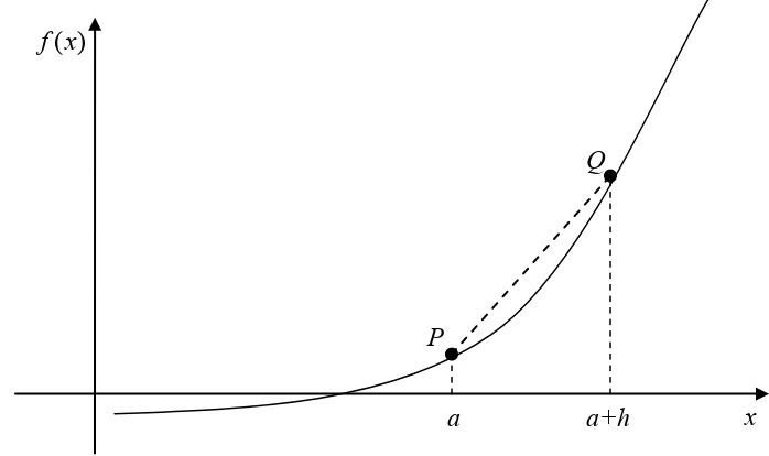
Let P and Q be two points on the curve as shown in Figure 1. The secant line is the straight line drawn through P and Q.
The slope of the secant line (Figure 2) is then given as
a h a
a f h a f mPQ
− +
− + =
) (
) ( ) (
secant ,
x P
Q
a a+h
) (x f
Figure 2 Calculation of the secant line. Q
P f(x)
x secant line
tangent line
h a f h a
f( + )− ( )
=
As Q moves closer and closer to P, the limiting portion is called the tangent line. The slope of the tangent line mPQ,tangent then is the limiting value of mPQ,secant as h→0.
h a f h a f m
h PQ
) ( ) ( lim
0 tangent ,
− + =
→
Example 1
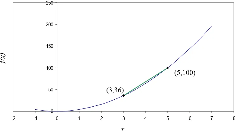
Find the slope of the secant line of the curve y =4x2 between points (3,36) and (5,100).
0 50 100 150 200 250
-2 -1 0 1 2 3 4 5 6 7 8
x
f(
x)
(5,100)
(3,36)
Figure 3 Calculation of the secant line for the function 2
4x y= . Solution
The slope of the secant line between (3,36) and (5,100) is
3 5
) 3 ( ) 5 (
− −
= f f
m
3 5
36 100
− − =
=32
Example 2
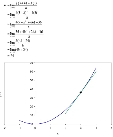
Find the slope of the tangent line of the curve y =4x2 at point (3,36). Solution
h
The slope of the tangent line is
h
Derivative of a Function
Recall from calculus, the derivative of a function f(x) at x=a is defined as
Solution
h
Solution
from knowing that
0
Second Definition of Derivatives
There is another form of the definition of the derivative of a function. The derivative of the function f(x) at x=a is defined as
a
of the definition of a derivative. Solution
Finding equations of a tangent line
One of the numerical methods used to solve a nonlinear equation is called the Newton-Raphson method. This method is based on the knowledge of finding the tangent line to a curve at a point. Let us look at an example to illustrate finding the equation of the tangent line to a curve.
Example 6
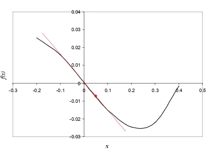
Find the equation of the line tangent to the function
4 3 0.165 3.993 10
)
(x =x − x+ × −
f at x=0.05.
Solution
The line tangent is a straight line of the form c
mx y = +
The tangent line passes through the point (0.05,−0.0077257), so
c c m
+ −
= −
+ =
−
) 05 . 0 ( 1575 . 0 0077257 .
0
) 05 . 0 ( 0077257 .
0
0001493 .
0
=
c
-0.03 -0.02 -0.01 0 0.01 0.02 0.03 0.04
-0.3 -0.2 -0.1 0 0.1 0.2 0.3 0.4 0.5
x
f(
x)
Figure 6 Graph of function f(x) and the tangent line at x = 0.05.
Hence,
c mx y = +
=−0.1575x+0.0001493
is the equation of the tangent line.
Other Notations of Derivatives
Derivates can be denoted in several ways. For the first derivative, the notations are
dx dy and y x f dx
d x
f′( ), ( ), ′,
For the second derivative, the notations are
2 2
2 2
, ), ( ), (
dx y d and y x f dx
d x
f ′′ ′′
n n n n
n n
dx y d y x f dx
d x
f( )( ), ( ), ( ),
Theorems of Differentiation
Several theorems of differentiation are given to show how one can find the derivative of different functions.
Theorem 1
The derivative of a constant is zero. If f(x)=k, where k is a constant, f′(x)=0.
Example 7
Find the derivative of f(x)=6. Solution
6 ) (x = f
0 )
( =
′ x f
Theorem 2
The derivative of f(x)= xn, where n≠0 is f′(x)=nxn−1. Example 8
Find the derivative of f(x)=x6. Solution
6
)
(x x
f =
1 6
6 )
( = −
′ x x
f
=6x5
Example 9
Find the derivative of f(x)=x−6. Solution
6
) (x =x− f
1 6
6 )
( =− −−
′ x x
f
=−6x−7 67
x
− =
Theorem 3
Example 10
Find the derivative of f(x)=10x6. Solution
6
10 )
(x x
f =
) 10 ( )
( x6
dx d x f′ =
10 x6
dx d
=
=10(6x5)
=60x5
Theorem 4
The derivative of f(x)=u(x)±v(x) is f′(x)=u′(x)±v′(x).
Example 11
Find the derivative of f(x)=3x3 +8. Solution
8 3 )
(x = x3 + f
) 8 3 ( )
( = 3 +
′ x
dx d x f
) 8 ( ) 3 ( 3
dx d x dx
d
+ =
0 ) (
3 3 +
= x
dx d
3(3 )
2
x
=
=9x2
Theorem 5 The derivative of
) ( ) ( )
(x u x v x
f =
is
) ( ) ( ) ( ) ( )
( u x
dx d x v x v dx
d x u x
f′ = + . (Product Rule)
Example 12
Solution
Using the product rule as given by Theorem 5 where,
)
Using the formula for the product rule
) The derivative of
2
Example 13
Find the derivative of
)
Solution
Use the quotient rule of Theorem 6, if
=9x2
Using the formula for the quotient rule,
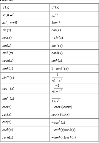
2 Table of Derivatives
) (x
coth 1−coth2(x)
) (
1
x csc−
1 | |
2
2 −
−
x x
x
) (
1 x
sec−
1 | |
2
2 −
x x
x
) (
1
x
cot− 2
1 1 x
+ −
x
a ln(a)ax
) (x ln
x
1
) (x loga
) ( 1 a xln
x
e ex
Chain Rule of Differentiation
Sometimes functions that need to be differentiated do not fall in the form of simple functions or the forms described previously. Such functions can be differentiated using the chain rule if they are of the form f(g(x)). The chain rule states
) ( )) ( ( )) ( (
(f g x f g x g x dx
d ′ ′
=
For example, to find f′(x) of f(x)=(3x2 −2x)4, one could use the chain rule. )
2 3 ( )
(x x2 x
g = −
g′(x)=6x−2
3
)) ( ( 4 )) (
(g x g x
f′ =
((3x2 −2x)4)=4(3x2 −2x)3(6x−2)
dx d
Implicit Differentiation
Sometimes, the function to be differentiated is not given explicitly as an expression of the independent variable. In such cases, how do we find the derivatives? We will discuss this via examples.
Example 14
Find dx dy
Solution
Example 15
If x2 −xy+y2 =5, find the value of y′. Solution
5
Higher order derivatives
So far, we have limited our discussion to calculating first derivative, f′(x) of a function
) (x
f . What if we are asked to calculate higher order derivatives of f(x).
is the velocity of the body, followed by the derivative of velocity with respect to time being the acceleration. Hence, the second derivative of the location function gives the acceleration function of the body.
Example 16
Given f(x)=3x3−2x−7, find the second derivative, f ′′(x) and the third derivative, f ′′′(x). Solution
Given
Example 17
If x2 −xy+ y2 =5, find the value of y′′. Solution
From Example 15 we obtain
After substitution of y′,
x y
x y
x y x
y x y
y
−
− − − − − −
= ′′
2
2 2 2 2 2
2 2
2
3 2 2
) 2 (
) (
6
x y
x xy y
− + − −
=
Finding maximum and minimum of a function
The knowledge of first derivative and second derivative of a function is used to find the minimum and maximum of a function. First, let us define what the maximum and minimum of a function are. Let f(x) be a function in domain D, then
) (a
f is the maximum of the function if f(a)≥ f(x) for all values of x in the domain D.
) (a
f is the minimum of the function if f(a)≤ f(x) for all values of x in the domain D. The minimum and maximum of a function are also the critical values of a function. An extreme value can occur in the interval [c,d] at
end points x=c,x=d.
a point in [c,d] where f′(x)=0.
a point in [c,d] where f′(x) does not exist.
These critical points can be the local maximas and minimas of the function (See Figure 8).
Example 18
Find the minimum and maximum value of f(x)=x2 −2x−5 in the interval [0,5].
maximum
minimum
x Figure 7 Graph illustrating the concepts of maximum and minimum.
Domain = [c,d]
Solution
5 2 )
(x =x2 − x−
f
2 2 )
( = −
′ x x
f
0 )
( =
′ x
f at x=1.
) (x
f′ exists everywhere in [0,5].
So the critical points are x=0, x=1, x=5. 5
) 0 ( 2 ) 0 ( ) 0
( = 2 − −
f =−5
5 ) 1 ( 2 ) 1 ( ) 1
( = 2 − −
f =−6
5 ) 5 ( 2 ) 5 ( ) 5
( = 2 − −
f =10
Hence, the minimum value of f(x) occurs at x=1, and the maximum value occurs at x=5. f(x)
●
●
●
●
● ●
●
x
Figure 8The plot shows critical points of f(x)in [c,d] .
Absolute Minimum
Local Minimum Local Minimum
Local Maximum (f´′(x) does not exist) Absolute Maximum
Local Maximum
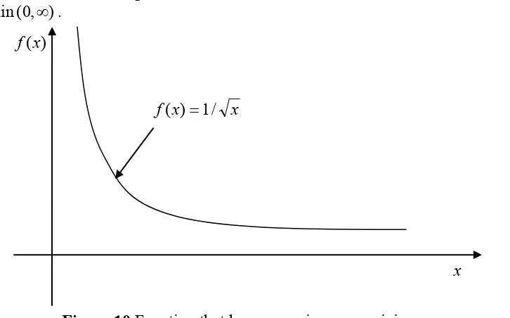
Figure 10 shows an example of a function that has no minimum or maximum value in the domain(0,∞).
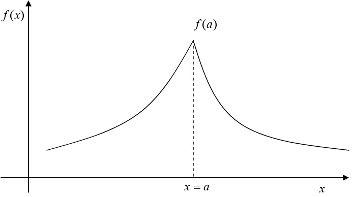
Figure 11 shows the maximum of the function occurring at a singular point. The function
) (x
f has a sharp corner at x=a.
x x
x f( )=1/ )
(x f
Figure 10 Function that has no maximum or minimum. -8
-6 -4 -2 0 2 4 6 8 10 12
0 1 2 3 4 5 6
x
f(
x)
minimum maximum
Example 19
Find the maximum and minimum of f(x)=2x in the interval [0,5]. Solution
x x f( )=2
2 )
( =
′ x f
0 )
( ≠
′ x
f on [0,5].
So the critical points are x=0 and x=5. x
x f( )=2
10 ) 5 ( 2 ) 5 (
0 ) 0 ( 2 ) 0 (
= =
= =
f f
So the minimum value of f(x)=2x is at x=0, and the maximum value is at x=5.
The point(s) where the second derivative of a function becomes zero is a way to know whether the critical point found in the first derivative test is a local minimum or maximum. Let f(x) be a function in the interval (c,d) and f(a)=0.
) (a
f is a local maximum of the function if f ′′(a)<0.
) (a
f is a local minimum of the function if f ′′(a)>0.
If f ′′(a)=0, then the second derivative does not offer any insight into the local maxima or minima.
Example 20
Remember Example 18 where we found f'(x)=0at x=1 for f(x)=x2 −2x−5 in the interval [0,5]. Is x=1 a local maxima or minima of the function?
) (x f
x
) (a f
a x=
Solution
5 2 )
(x =x2 − x− f
2 2 )
( = −
′ x x f
0 )
( =
′ x
f at x=1
0 2 ) 1 (
2 ) (
> = ′′
= ′′
f x f
So the f(1) is the local minimum of the function.
Applications of Derivatives
Below are some examples to show real-life applications of differentiation.
Example 21
A rain gutter cross-section is shown below.
What angle of θ would make the cross-sectional area of ABCD maximum? Note that common sense or intuition may lead us to believe that θ =π/4 would maximize the cross-sectional area of ABCD. Question your intuition.
Solution
CE AD BC
Area= ( + )× 2
1
) (θ
sin CD CE =
=3sin(θ)
BC =3
) ( )
cos(θ ABcos θ CD
BC
AD= + +
) ( 3 ) ( 3
3 cosθ cosθ
AD= + +
) ( 6 3 cos θ AD= +
)) ( 3 ))( ( 6 3 3 ( 2
1 θ θ
sin cos
Area= + + A
θ
3
B C
D E
θ
3
3
=9sin(θ)+9sin(θ)cos(θ)
Example 22
A classic example of the application of differentiation is to find the dimensions of a circular cylinder for a specific volume but which uses the least amount of material. Do this classic problem for a volume of 9m3.
Solution
2 2
9 9
r h
h r
π π
= =
This gives the surface area just in terms of r as
+ =
2
2 9
2 2
r r r
A
π π π
1 2
2
18 2
18 2
−
+ =
+ =
r r
r r
π π
To find the minimum, take the first derivative of A with respect to r as
2
) 1 ( 18
4 + − −
= r r
dr
dA π
4 182
r r−
= π
Solving for
0
=
dr dA
,
0 18 4
0 18 4
3 2
= −
= −
r r r
π π
π
4 18
3 =
r
Figure 13 Cylinder drawing for Example 20. r
h
3
m 9
=
m 12725 . 1
4
18 3
1
= =
π
r
Since
2
9
r h
π = ,
2
) 12725 . 1 (
9
π =
h
=2.25450m
But does this value of r correspond to a minimum?
3 2
2
) 2 ( 18
4 − − −
= r
dr A
d π
5025 . 44
12725 . 1
36 4
36 4
3
= + =
+ =
π π
r
This value 2 0
2 >
dr A d
for r =1.12725m. As per the second derivative test, r=1.12725m
corresponds to a minimum.
DIFFERENTIATION
Topic Primer on Differentiation
Summary These are textbook notes of a primer on differentiation
Major General Engineering
Authors Autar Kaw, Luke Snyder
Date July 17, 2008