PROGRAMMING
ILAN ADLER, NARENDRA KARMARKAR, MAURICIO G.C. RESENDE, AND GERALDO VEIGA
ABSTRACT. This paper describes the implementation of power series dual affine scaling variants of Karmarkar’s algorithm for linear programming. Based on a continuous version of Karmarkar’s algorithm, two variants resulting from first and second order approxima-tions of the continuous trajectory are implemented and tested. Linear programs are ex-pressed in an inequality form, which allows for the inexact computation of the algorithm’s direction of improvement, resulting in a significant computational advantage. Implementa-tion issues particular to this family of algorithms, such as treatment of dense columns, are discussed. The code is tested on several standard linear programming problems and com-pares favorably with the simplex code MINOS 4.0.
1. INTRODUCTION
We describe in this paper a family of interior point power series affine scaling algo-rithms based on the linear programming algorithm presented by Karmarkar (1984). Two algorithms from this family, corresponding to first and second order power series approxi-mations, were implemented in FORTRAN over the period November 1985 to March 1986. Both are tested on several publicly available linear programming test problems (Gay 1985). We also test one of the algorithms on randomly generated multi-commodity network flow problems (Ali & Kennington 1977) and on timber harvest scheduling problems (Johnson 1986).
Several authors (see, e.g., Aronson, Barr, Helgason, Kennington, Loh & Zaki (1985), Lustig (1985), Tomlin (1987) and Tone (1986)) have compared implementations of inte-rior point algorithms with simplex method codes, but have been unable to obtain compet-itive solution times. An implementation of a projected Newton’s barrier method reported by Gill, Murray, Saunders, Tomlin & Wright (1986) presents the first extensive computa-tional evidence indicating that an interior point algorithm can be comparable in speed with the simplex method.
In our computational experiments, solution times for the interior point implementations are, in most cases, less than those required by MINOS 4.0 (Murtagh & Saunders 1977). Furthermore, we are typically able to achieve 8 digit accuracy in the optimal objective func-tion value without experiencing the numerical difficulties reported in previous implemen-tations.
MINOS is a FORTRAN code intended primarily for the solution of constrained non-linear programming problems, but includes an advanced implementation of the simplex
Date: 14 March 1989 (Revised May 25 1995).
Key words and phrases. Linear programming, Karmarkar’s algorithm, Interior point methods.
This article originally appeared in Mathematical Programming 44 (1989), 297–335. An errata correcting the description of the power series algorithm was published in Mathematical Programming 50 (1991), 415. The ver-sion presented here incorporates these corrections to the body of the article. In addition, we updated references to some articles published in final form after the publication of this paper. We request that authors refer to this article by its original bibliographical reference.
method. An updated version, MINOS 5.0 (Murtagh & Saunders 1983), features a scal-ing option and an improved set of routines for computscal-ing and updatscal-ing sparse LU factors. This latest version of MINOS was not available at the University of California, Berkeley, where the computational tests described in this paper were carried out. We believe that for the purposes of this study, MINOS 4.0 constitutes a reasonable benchmark simplex imple-mentation. Furthermore, as evidenced by the results reported in Gill et al. (1986) we do not expect MINOS 5.0 to perform significantly faster for the test problems considered here.
The plan of the paper is as follows. In Section 2, we describe our Algorithm I, a ba-sic interior point method, commonly referred to as the affine scaling algorithm. When Al-gorithm I takes infinitesimal steps at each iteration, the resulting continuous trajectory is described by a system of differential equations. In Section 3, we discuss the family of al-gorithms constructed by truncating the Taylor expansion representing the solution of this system of differential equation. A first order approximation to the Taylor expansion results in Algorithm I. We also implement Algorithm II, which is obtained by truncating the Taylor expansion to a second order polynomial. We show in Section 4 how an initial interior so-lution can be obtained and in Section 5 how the algorithms can be applied to general linear programming problems. In Section 6, we describe the stopping criterion used in the compu-tational experiments. Section 7 discusses some implementation issues, including symbolic and numerical factorizations, using an approximate scaling matrix, reducing fill-in during Gaussian elimination and using the conjugate gradient algorithm with preconditioning to solve problems with dense columns. In Section 8, we report the computational results of running the algorithms on three sets of test problems. The first set is a family of publicly available linear programs from a variety of sources. The others are, respectiv ely, randomly generated multi-commodity network flow problems and timber harvest scheduling prob-lems. We compare these results to those of the simplex code MINOS 4.0 and for the case of the multi-commodity network flow problems to MCNF85 a specialized simplex based code for multi-commodity network flow (Kennington 1979). Conclusions are presented and future research is outlined in Section 9.
2. DESCRIPTION OFALGORITHM Consider the linear programming problem:
P: maximize cTx (2.1)
subject to: Ax≤b (2.2)
where c and x are n-vectors, b an m-vector and A is a full rank m×n matrix, where m≥n and c6=0. In assumptions relaxed later, we require P to have an interior feasible solution x0.
Rather than expressing P in the standard equality form, we prefer the inequality formu-lation (2.1) and (2.2). As discussed later in this section, there are some computational ad-vantages in the selection of search directions under this formulation. In Section 5, we show how to apply this approach to linear programs in standard form.
classified as dual affine scaling algorithms. However, these algorithms are equivalent to their primal counterparts applied to problems in inequality form.
Starting at x0, the algorithm generates a sequence of feasible interior points{x1,x2, . . . ,xk, . . .}
with monotonically increasing objective values, i.e.,
b−Axk>0 (2.3)
cTxk+1>cTxk,
(2.4)
terminating when a stopping criterion to be discussed later is satisfied. Introducing slack variables to the formulation of P, we have:
P: maximize cTx (2.5)
subject to: Ax+v=b (2.6)
v≥0,
(2.7)
where v is the m-vector of slack variables.
Affine variants of Karmarkar’s algorithm consist of a scaling operation applied to P, fol-lowed by a search procedure that determines the next iterate. At each iteration k, with vk and xkas the current iterates, a linear transformation is applied to the solution space,
ˆ
v=D−v1v,
(2.8)
where
Dv=diag(vk1, . . . ,vkm).
(2.9)
The slack variables are scaled so that xk is equidistant to all hyperplanes generating the closed half-spaces whose intersection forms the transformed feasible polyhedral set,
{x∈ℜn|Dv−1Ax≤D−v1b}.
(2.10)
Rewriting equations (2.1) and (2.2) in terms of the scaled slack variables, we have ˆ
P: maximize cTx (2.11)
subject to Ax+Dvvˆ=b
(2.12)
v≥0 (2.13)
The set of feasible solutions for P is denoted by
X={x∈ℜn|Ax≤b}
(2.14)
and the set of feasible scaled slacks in ˆP is
ˆ
V={vˆ∈ℜm| ∃x∈X,Ax+Dvvˆ=b}.
(2.15)
As observed in Gonzaga (1991), under the full-rank assumption for A, there is a one to one relationship between X and ˆV , with
ˆ
v(x) =D−v1(b−Ax)
(2.16)
and
x(vˆ) = (ATD−v2A)−1ATD−v1(D−v1b−ˆv).
(2.17)
There is also a corresponding one to one relationship linking feasible directions hxin X and
hˆvin ˆV, with
hˆv=−D−v1Ahx
and
hx=−(ATD−v2A)−1ATD−v1hˆv.
(2.19)
Observe from (2.18) that a feasible direction in ˆV lies on the range space of D−v1A. As in other presentations of affine variants of Karmarkar’s algorithm, the search direc-tion selected at each iteradirec-tion is the projected objective funcdirec-tion gradient with respect to the scaled variables. Since only the slack variables are changed by the affine transformation, using (2.11) and (2.17), we can compute the gradient of the objective function with respect to ˆv,
∇ˆvc(x(vˆ)) = (∇ˆvx(vˆ))T∇xc(x) =−D−v1A(ATD−v2A)−1c.
(2.20)
The gradient with respect to the scaled slacks lies on the range space of D−v1A, making a
projection unnecessary. Consequently, the search direction in ˆv is
hˆv=−D−v1A(ATD−v2A)−1c,
(2.21)
and from (2.19) the corresponding feasible direction in X can be computed,
hx= (ATD−v2A)−1c.
(2.22)
Applying the inverse affine transformation to hvˆ, we obtain the corresponding feasible direction for the unscaled slacks,
hv=−A(ATDv−2A)−1c.
(2.23)
Under the assumption that c6=0, unboundedness is detected if hv≥0. Otherwise, the next
iterate is computed by taking the maximum feasible step in the direction hv, and retracting
back to an interior point according to a safety factorγ, 0<γ<1, i.e.,
xk+1=xk+αhx,
(2.24)
where
α=γ×min{−vki/(hv)i|(hv)i<0,i=1, . . . ,m}.
(2.25)
The above formulation allows for inexact projections without loss of feasibility. Even if hxis not computed exactly in (2.22), a pair of feasible search direction can still be obtained
by computing
hv=−Ahx.
(2.26)
Given an interior feasible solution x0, a stopping criterion and a safety factorγ, Pseudo-code 2.1 describes Algorithm I as outlined in this section. As in subsequent instances in this paper, algorithms are expressed in an Algol-like algorithmic notation described by Tarjan (1983).
3. A FAMILY OFINTERIOR-POINTALGORITHMS USINGPOWERSERIESAPPROXIMATIONS
Consider the continuous trajectory generated by Algorithm I when infinitesimal steps are taken at each iteration (Bayer & Lagarias 1989). Let us denote the path of interior feasible solutions for P by(x¯(τ),v¯(τ)), where the real parameterτis the continuous counterpart to the iteration counter. For any value ofτ, the corresponding search directions hx(¯ τ)and hv(¯ τ) can be computed by expressions (2.22) and (2.23). Alternatively, the search directions can be described by an equivalent system of linear equations,
1. procedure Algorithm I (A, b, c, x0, stopping criterion,γ) 2. k :=0;
3. do stopping criterion not satisfied→
4. vk:=b−Axk;
5. Dv:=diag(vk1, . . . ,vkm);
6. hx:= (ATD−v2A)−1c;
7. hv:=−Ahx;
8. if hv≥0→return fi;
9. α:=γ×min{−vki/(hv)i|(hv)i<0,i=1, . . . ,m}; 10. xk+1:=xk+αhx;
11. k :=k+1; 12. od
13. end Algorithm I
Pseudo-code 2.1: Algorithm I
Ahx¯(τ)+hv¯(τ)=0. (3.2)
By taking infinitesimal steps, the resulting continuous trajectory is such that
d ¯x
dτ(τ) =hx¯(τ) and d ¯v
dτ(τ) =hv¯(τ). (3.3)
Given the system of linear equations (3.1) and (3.2), we replace the search directions by the corresponding derivatives with respect to the trajectory parameter, resulti ng in the system of nonlinear, first order differential equations
−ATD−v¯(2τ)d ¯v dτ(τ) =c (3.4)
Ad ¯x dτ(τ) +
d ¯v
dτ(τ) =0, (3.5)
with the boundary conditions
¯
x(0) =x0 and v¯(0) =v0,
(3.6)
where the initial solution(x0,v0)is given and satisfies Ax0+v0=b, v0>0.
By following the trajectory satisfying (3.4)–(3.6) we can, theoretically, obtain the opti-mal solution to P (Adler & Monteiro 1991). In practice, we build an iterative procedure where, after replacing the current iterate for the initial solution in the boundary condition, an approximate solution to (3.4)–(3.6) is computed, using a truncated Taylor power series expansion. The next iterate is determined through a search on the approximate trajectory.
As discussed later in this section, the search procedure requires a suitable reparametri-zation of the continuous trajectory,
τ=ρ(t),
(3.7)
whereρ(t)is a monotonically increasing, infinitely differentiable real function such that
x(t) =x¯(ρ(t)) and v(t) =v¯(ρ(t)).
(3.8)
Reparametrizing (3.4)–(3.6), we have
−ATD−v(2t)dv dt(t) =
Adx
Since we cannot compute an exact solution to (3.9)–(3.11), we use approximate solu-tions to the system of differential equasolu-tions as the backbone of a family of iterative al-gorithms. At each iteration k, the algorithm restarts the trajectory with an initial solution
(x(0),v(0)) = (xk−1,vk−1). A new iterate is generated by moving on the approximate tra-jectory without violating nonnegativity of the slack variables. The approximate solutions can be computed by means of a truncated Taylor expansion of order r (Karmarkar, Lagarias, Slutsman & Wang 1989), such that for t>0,
x(t)≈x˜(t) =x(0) +
Applying Leibniz’s differentiation theorem to the product F(t)G(t), we have
i
From (3.16), the derivatives of F(t)can be computed recursively by
diF
Taking derivatives of both sides of (3.9), and rewriting the left hand side of the equation in terms of F(t), we have
In an implementable reformulation of (3.19) and (3.20), we eliminate the binomial terms
Solving (3.19) and (3.20), we have
zxi =ρi(ATDv−(20)A)−
The approximate trajectory based on a power series of order r is rewritten as
˜
At iteration k, the next iterate is computed as
xk+1=x˜(α) and vk+1=v˜(α),
By selecting a suitable reparametrizationρ(t), the line search on ˜v(t)that computesα in (3.28) can be limited to the interval 0≤t ≤1. Since ˜x(t)and ˜v(t)depend solely on derivatives ofρ(t)evaluated at t =0, the desired reparametrization is fully characterized by constantsρ1, . . . ,ρr. Values forρiare computed by selecting a row index l, and forcing
From (3.24) and (3.25), we have
z1x=ρ1h1x and z1v=ρ1h1v.
Once again, under the assumptions that A is full rank and c6=0, unboundedness is de-tected if hv≥0. Otherwise, we determine the row index l by performing a ratio test between
v(0)and search direction h1v, i.e.,
l=argmin 1≤i≤m
{−v(0)/(h1v)i|(h1v)i<0}.
(3.34)
This operation corresponds to searching along the first order approximation of trajectory v(t). From the conditions imposed on the reparametrization by (3.30), the truncated Taylor expansion in (3.26) is such that
˜
vl(1) =v(0) +ρ1h1v,
(3.35)
and from (3.29) and (3.33), we compute
ρ1=−vl(0)/(h1v)l.
(3.36)
Iteratively, for i=2, . . . ,r, we computeρi, zixand ziv. Based on (3.24) and (3.25),
zix=ρih1x+hix and ziv=−Azix.
(3.37)
where
hix= (ATD−v(20)A)
−1 ATD−v(10)
i−1
∑
j=1
Fi−jzvj and hiv=−Ahix.
(3.38)
To satisfy (3.30), we have
ρi=−(hiv)l/(h1v)l.
(3.39)
Pseudo-code 3.1 formalizes the algorithm based on a truncated power series of order r. The computational experiments reported in Section 8 include Algorithm II, which is the second order version of this algorithm. In a practical implementation, the additional com-putational effort, when compared to Algorithm I, is dominated by the solution of systems of symmetric linear equations to compute hixfor i=2, . . . ,r. As in Algorithm I, if ˜x(t)is
not obtained exactly, a pair of feasible trajectories can still immediately available. By com-puting
ziv=−Azix for i=1, . . . ,r,
(3.40)
we guarantee that(x˜(t),v˜(t))is a feasible for 0≤t≤α, where 0≤α≤1 is the maximum feasible step.
4. INITIALSOLUTION
Algorithm I and the truncated power series algorithms require that an initial interior so-lution x0be provided. Since such solution does not necessarily exist for a generic linear program, and a starting solution close to the faces of the feasible polyhedral set can imply in very slow convergence (Megiddo & Shub 1989), we propose a Phase I/Phase II scheme, where we first solve an artificial problem with a single artificial variable having a large cost coefficient assigned to it.
Firstly, we compute a tentative solution for P,
x0= (kbk2/kAck2)c. (4.1)
For the computational experiments reported in Section 8, we compute the initial value for the artificial variable as
x0a=−2×min{(b−Ax0)i|i=1, . . . ,m}.
1. procedure PowerSeries(A, b, c, x0, stopping criterion,γ, r) 2. k :=0;
3. do stopping criterion not satisfied→
4. x(0):=xk; 5. v(0):=b−Ax(0);
6. Dv(0):=diag(v1(0), . . . ,vm(0)); 7. h1x:= (ATDv(0)−2A)−1c; h1
v:=−Ah1x;
8. if h1
v≥0 return fi;
9. l :=argmin1≤i≤m{−v(0)/(h1v)i|(h1v)i<0};
10. ρ1:=−vl(0)/(h1v)l;
11. z1x:=ρ1h1x; z1v:=ρ1h1v;
12. F1:=Dv(0)−2z1
v;
13. for i=2, . . . ,r→
14. hix:= (ATDv(0)−2A)−1ATDv(0)−1∑i−j=11Fi−jz
j v;
15. hi
v:=−Ahix;
16. ρi:=−(hiv)l/(h1v)l;
17. zix:=ρih1x+hix; ziv:=−Azix;
18. Fi:=Dv(0)−2ziv−Dv(0)−1∑ j=1
i−1Fi−jz
j v;
19. rof;
20. x˜(t):=x(0) +∑r
i=1tizix; ˜v(t):=v(0) +∑ri=1tiziv;
21. α:=γ×sup{t|0≤t≤1,v˜i(t)≥0,i=1, . . . ,m}; 22. xk+1:=x˜(α);
23. k :=k+1; 24. od
25. end PowerSeries
Pseudo-code 3.1: Power Series Algorithm
Although it did not occur in any of the test problems reported in this paper, the com-putation in (4.2) can be such that x0a≈0. Consequently, for application to generic linear
programs, we recommend an alternative computation of the initial value of the artificial variable,
x0a=2× kb−Ax0k2. (4.3)
The n+1-vector(x0,x0a)is an interior solution of the Phase I linear programming
prob-lem
Pa: maximize cTx−Mxa
(4.4)
subject to: Ax−exa≤b
(4.5)
where
e= (1,1, . . . ,1)T.
(4.6)
The large artificial cost coefficient is computed as a function of the problem data,
M=µ×cTx0/x0a,
(4.7)
whereµis a large constant.
Initially, the algorithm is applied to Pawith a modified stopping criterion. In this Phase I
exists, finds a solution that satisfies the stopping criterion for problem P. Withεf defined as
the feasibility tolerance, the modified stopping criterion for Phase I is formulated as follows: (i) If xka<0 at iteration k, then xkis an interior feasible solution for problem P.
(ii) If the algorithm satisfies the regular stopping criterion and xk
a>εf, P is declared
in-feasible.
(iii) If the algorithm satisfies the regular stopping criterion and xka<εf, either
unbounded-ness is detected or an optimal solution is found. In this case, P has no interior feasible solution.
If Phase I terminates according to condition (i), the algorithm is applied to problem P starting with the last iterate of Phase I and using the regular stopping criterion.
5. APPLICATION TO THEGENERALLINEARPROGRAMMINGPROBLEM It is not common practice to formulate a linear programming problem as in (2.1) and (2.2). Instead, a standard form is usually preferred,
LPP: minimize bTy (5.1)
subject to: ATy=c (5.2)
y≥0 (5.3)
where A is an m×n matrix, c an n-vector and b and y m-vectors. The dual linear program-ming problem of (5.1)–(5.3), however, has the desired form:
LPD: maximize cTx (5.4)
subject to: Ax≤b (5.5)
where x is an n-vector. Note that LPD is identical to P, as defined in (2.1) and (2.2). At iteration k, with current solutions xkand vk, a tentative dual solution is defined as
yk=D−v2A(ATD−v2A)−1c, (5.6)
where
Dv=diag(vk1, . . . ,vkm).
(5.7)
This computation of the tentative dual solution, similar to the one suggested by Todd & Burrell (1986), can be performed by scaling the first order search direction in each iteration of the algorithm. From (2.23), for iteration k,
yk=D−v2hv.
(5.8)
The tentative dual solution minimizes the deviation from complementary slackness with respect to the current iterate xk, relaxing the nonnegativity constraints (5.3) (Chandru & Kochar 1985). Formally, consider the problem
minimize
m
∑
j=1
(vkjyj)2
(5.9)
subject to: ATy=c.
(5.10)
a sequence of feasible primal solutions converging to an optimal solution, the corresponding sequence of tentative dual estimates also converges to the optimal dual solution.
6. STOPPINGCRITERION
In the computational experiments reported in this study, both Algorithms I and II are terminated whenever the relative improvement to the objective function is small, i.e.,
|cTxk−cTxk−1|/max{1,|cTxk−1|}<ε,
(6.1)
whereεis a given small positive tolerance.
The tentative dual solution yk, computed in (5.6), can be used to build an alternative stop-ping criterion. If ykand vksatisfy
ATyk=c,
(6.2)
yk≥0,
(6.3)
ykjvkj=0,j=1,2, . . . ,m,
(6.4)
then, by duality theory of linear programming, ykis optimal for LPP and xkis optimal for
LPD. Since (6.2) is automatically satisfied, a stopping criterion, replacing (6.1), is such that
the algorithm terminates whenever
ykj≥ −ε1kykk2, j=1,2, . . . ,m, (6.5)
and
|ykjvkj| ≤ε2kykk2kvkk2, j=1,2, . . . ,m, (6.6)
for given small positive tolerancesε1 andε2. The relations in (6.5) and (6.6) serve as a verification that xkand ykare indeed approximate optimal solutions for LPD and LPP, re-spectively.
Unboundedness of LPD is, theoretically, detected by the algorithm whenever hv≥0, i.e.,
the ratio tests in (2.25) and (3.34), involving the first order search direction fail. In practice, an additional test is required, LPD is declared unbounded whenever the objective function value exceeds a supplied bound.
7. IMPLEMENTATIONISSUES
In this section, we briefly discuss some important characteristics of this implementation. A detailed description of the data structures, programming techniques and used in the im-plementation of Algorithms I and II is the subject of Adler, Karmarkar, Resende & Veiga (1989).
7.1. Computing Search Directions. As in other variants of Karmarkar’s algorithm, the main computational requirement of the algorithms described in this paper consists of the solution of a sequence of sparse symmetric positive definite systems of linear equations de-termining the search directions for each iteration. In Algorithm I, for each iteration k, a linear trajectory is determined by the feasible direction computed in
Bkhx=c,
(7.1.1)
with
Bk=ATD−v2A,
where
Dv=diag(vk1, . . . ,vkm).
(7.1.3)
Under the full-rank assumption for A, the system of linear equations in (7.1.1) is sym-metric and positive definite. Such systems of linear equations are usually solved by means of the LU factorization,
Bk=LU,
(7.1.4)
where L is an m×m unit lower triangular matrix (a matrix that has exclusively ones in its main diagonal), and U is an m×m upper-triangular matrix. In the case of positive definite matrices, this LU factorization always exists and is unique. Furthermore, if the system is also symmetric, the factor L can be trivially obtained from U with
L=D−U1UT,
(7.1.5)
where DU is a diagonal matrix with elements drawn from the diagonal of U. Rewriting
(7.1.1), we have
(LU)hx=c.
(7.1.6)
Direction hxin (7.1.6) can be determined by solving two triangular systems of linear
equa-tions, performing a forward substitution
Lz=c,
(7.1.7)
followed by a back substitution
Uhx=z.
(7.1.8)
In each iteration of the higher order algorithms described in Section 3, the additional di-rections in (3.38) also involve the solution of linear systems identical to (7.1.1), except for different right-hand sides. Solving these additional systems of linear equations involve only the back and forward substitution operations, using the same LU factors. Furthermore, dur-ing the execution of the algorithm only Dvchanges in (7.1.2), while A remain unaltered.
Therefore, the nonzero structure of ATD−2
v A is static throughout the entire solution
proce-dure. An efficient implementation of the Gaussian elimination procedure can take advan-tage of this property by performing, in the beginning of the algorithm, a single symbolic factorization step, i.e., operations that depend solely on the nonzero structure of the system matrix. For example, at this stage of the algorithm, we determine the nonzero structure of LU factors and build a list of the numerical operations performed during the Gaussian elim-ination procedure. At each iteration k of the algorithm, the actual numerical values of Bkare
computed and incorporated in the symbolic information. Next, the numerical factorization is executed, by traversing the list of operations, yielding the LU factors.
7.2. Using an Approximate Scaling Matrix. Based on the theoretical approach suggested by Karmarkar (1984), a significant reduction in the computational effort can be achieved by using an approximate scaling matrix when computing the numerical values for matrix Bk
at each iteration. The matrix for the system of linear equations in (7.1.1) is replaced by
˜
Bk=ATD˜−k2A,
(7.2.1)
where ˜Dkis an approximate scaling matrix, computed by selectively updating the scaling
is computed as follows:
˜ Dk(i,i) =
( ˜
Dk−1(i,i) if|Dv(i,i)−D˜k−1(i,i)|/D˜k−1(i,i)<δ Dv(i,i) if|Dv(i,i)−D˜k−1(i,i)|/D˜k−1(i,i)≥δ (7.2.2)
for a givenδ>0. After computing the current approximate scaling matrix according to 7.2.2, we define
∆=D˜−2
k −D˜
−2
k−1. (7.2.3)
Then, we have the update expression ˜
Bk=B˜k−1+AT∆A. (7.2.4)
This enables us to update the linear system matrix by rescaling only a reduced set of columns of AT.
7.3. Ordering for Sparsity. When a sparse matrix is factored, fill-in usually occurs. The triangular factors contain nonzero elements in positions where Bk has zeros. Fill-in
de-grades the performance of the sparse Gaussian elimination used to compute the LU factor-ization, also affecting the back and forward substitution operations. It is possible to reduce fill-in by performing a permutation of columns and rows in Bk.
If P is a permutation matrix, then 7.1.1 and
(PBkPT)Phx=Pc
(7.3.1)
are equivalent systems. Furthermore, there exists a permutation matrix ¯P such that the fill-in generated fill-in the triangular factors is mfill-inimized. Unfortunately, ffill-indfill-ing this permutation matrix is an NP-complete problem (Yannakakis 1981). However, the minimum degree and minimum local fill-in ordering heuristics (Rose 1972) have been shown to perform well in practice (Duff, Erisman & Reid 1986). We use either the minimum degree heuristic as im-plemented in subroutine MD of the Yale Sparse Matrix Package (Eisenstat, Gurshy, Schultz & Sherman 1982), or the minimum local fill-in implementation in deCarvalho (1987).
7.4. Treating Dense Columns in the Coefficient Matrix. In the presence of a few dense columns in AT, ATD−2
v A will be impracticably dense, regardless of the permutation matrix.
Consequently, we face prohibitively high computational effort and storage requirements during Gaussian elimination. To remedy this situation, we make use of a hybrid scheme in which we first perform an incomplete factorization of ATD−2
v A. Next, we use the
in-complete Cholesky factors as preconditioners for a conjugate gradient method to solve the system of linear equations defined in 7.1.1.
Let(N,N¯)be a partition of the column indices of AT, such that the columns of AT
Nhave
density smaller than a given parameterλ. At iteration k, the incomplete Cholesky factors ˜Lkand ˜LTk are such that
ATND−v2AN=˜Lk˜LTk .
(7.4.1)
Using the conjugate gradient algorithm, we solve the system of linear equations
Qu=f,
(7.4.2)
where
Q=˜L−1
k (A TD−2
v A)(˜LTk)−1,
(7.4.3)
and
f =˜L−k1c.
The search direction hxis computed by performing a back substitution operation, solving
u=˜LT khx.
(7.4.5)
Given a termination toleranceεcg >0, the conjugate gradient algorithm is outlined in
Pseudo-code 7.4.1.
1. procedure ConjugateGradient(Q, f ,εcg)
2. u0:=f ; 3. r0:=Qu0−f ; 4. p0:=−r0; 5. i :=0; 6. dokrik2
2≥εcg→
7. qi:=Qpi;
8. αi:=krik22/pTiqi;
9. ui+1:=ui+αipi;
10. ri+1:=Qui+1−f ; 11. βi:=kri+1k22/krik22; 12. pi+1:=−ri+1+βipi;
13. i :=i+1; 14. od
15. end ConjugateGradient
Pseudo-code 7.4.1: Conjugate Gradient Algorithm
8. TESTPROBLEMS
In this section, we report the computational results of running our implementations of Al-gorithms I and II on a set of linear programming test problems (Gay 1985) available through NETLIB (Dongarra & Grosse 1987). NETLIB is a system designed to provide efficient distribution of public domain software to the scientific community through computer net-works, e.g. Arpanet, UNIX UUCP network, CSNET Telenet and BITNET. We also report the results of running Algorithm I on linear programs generated by two models. The first set is composed of randomly generated multi-commodity network flow problems gener-ated with MNETGN (Ali & Kennington 1977). The other is a collection of timber har-vest scheduling problems generated by FORPLAN (Johnson 1986), a linear programming based system used for long-range planning by the US Forest Service.
8.1. The NETLIB Test Problems. This collection of linear programs consists of prob-lems contributed by a variety of sources. It includes linear programming test probprob-lems from the Systems Optimization Laboratory at Stanford University, staircase linear programs gen-erated by Ho & Loute (1981), and many real world problems. We considered in our tests all of the available problems that do not have a BOUNDS section in their MPS representation, since the current version of our code cannot handle bounded variables implicitly.
TABLE8.1.1. NETLIB test problem statistics
Problem Rows Columns nonz(A) nonz((PA)TPA)a nonz(L)
Afiro 27 51 102 90 107
ADLittle 56 138 424 377 404
Scagr7 129 185 465 606 734
Sc205 205 317 665 654 1182
Share2b 96 162 777 871 1026
Share1b 117 253 1179 967 1425
Scorpion 388 466 1534 1915 2324
Scagr25 471 671 1725 2370 2948
ScTap1 300 660 1872 1686 2667
BrandY 220 303 2202 2190 2850
Scsd1 77 760 2388 1133 1392
Israel 174 316 2443 3545 3707
BandM 305 472 2494 2929 4114
Scfxm1 330 600 2732 3143 4963
E226 223 472 2768 2683 3416
Scrs8 490 1275 3288 1953 5134
Beaconfd 173 295 3408 1720 1727
Scsd6 147 1350 4316 2099 2545
Ship04s 402 1506 4400 2827 3134
Scfxm2 660 1200 5469 6306 9791
Ship04l 402 2166 6380 4147 4384
Ship08s 778 2467 7194 3552 4112
ScTap2 1090 2500 7334 6595 14870
Scfxm3 990 1800 8206 9469 14619
Ship12s 1151 2869 8284 4233 5063
Scsd8 397 2750 8584 4280 5879
ScTap3 1480 3340 9534 8866 19469
CzProb 929 3340 10043 6265 6655
25FV47b 821 1876 10705 10919 33498
Ship08l 778 4363 12882 6772 7128
Ship12l 1151 5533 16276 8959 9501
aUsing the minimum degree ordering heuristic. b25FV47 is also known as BP822.
Column 6 gives the nonzero elements in the Cholesky factor. The fill-in is the difference between columns 6 and 5. The entries in columns 5 and 6 for problem Israel are those used by the algorithm, i.e., after 6 dense columns of AT are dropped.
the FORTVS compiler with compiler options OPT(3), NOSYM and NOSDUMP The re-ported CPU times were computed with utility routine DATETM taking into account pre-processing (e.g. input matrix cleanup, ordering and symbolic factorization) and all oper-ations until termination. However, they exclude the effort required to translate the linear programs from MPS format.
Execution times for Algorithm I and Algorithm II are compared to those of the simplex code MINOS 4.0 The reported CPU times for MINOS are those of subroutine DRIVER which also excludes the time to read and translate the MPS input file. The results of solving the NETLIB test problems by MINOS 4.0 are displayed in Table 8.1.2. In running MI-NOS we use default parameters except for LOG FREQ= 200 and ITERATIONS= 7500. The problem size parameters, ROWS, COLUMNS and ELEMENTS were set to the exact number of rows, columns and nonzero elements of the coefficient matrix. In this fashion, MINOS selects the value for the all important PARTIAL PRICE parameter according to its built-in default strategy. Using the default parameters, MINOS 4.0 achieved 7 digit accu-racy on all problems, if compared to the optimal objective values reported in Gay (1985).
Since the NETLIB test problems are not in the form described by 2.1 and 2.2, Algo-rithms I and II solve the corresponding dual linear programming problems. A primal opti-mal solution is obtained from 5.6, involving the last scaling matrix Dvand the last search
direction for the dual slacks. By contrast MINOS solves the test problems is its original form. Tables 8.1.3 and 8.1.4 summarize computational results for Algorithm I on the set of test problems, using, respectively, the minimum degree and the minimum local fill-in or-dering heuristics. Table 8.1.5 presents results for Algorithm II, which uses the minimum degree ordering heuristic.
Both Algorithms I and II were tested with the following parameter settings. The safety factor parameter was set toγ=0.99 for the first 10 iterations andγ=0.95 thereafter. Both algorithms were terminated when the relative improvement in the objective function fell belowε=10−8. In Phase I, the value of the artificial variable cost defined in 4.7 was de-termined by the constantµ=105. The diagonal update tolerance was set toδ=0.1 and the column density parameter for building the incomplete Cholesky factorization in the conju-gate gradient algorithm was set toλ=0.3.
Table 8.1.6 compares execution times for the three algorithms. CPU times displayed for MINOS and Algorithm I were measured on the IBM 3090 while those for Algorithm II are from the IBM 3081-K For the sake of consistency, when computing the CPU times ratio between MINOS and Algorithm II, the execution times for MINOS are those of the IBM 3081-K Figures 8.1.1 and 8.1.2 illustrate graphically the performances of MINOS and Algorithm I.
Table 8.1.7 focuses on five subgroups of problems, where each subgroup is made up of problems having the same structure, or generated by the same model. In this table, ratios of MINOS iterations to Algorithm I iterations, MINOS CPU time per iteration to Algorithm I CPU time per iteration and MINOS total CPU time to Algorithm I total CPU time are given.
Table 8.1.8 presents detailed results related to the generation of primal solutions in Algo-rithm I. Let t be the number of iterates generated by the algoAlgo-rithm. The normalized duality gap
|bTyt−cTxt|/|btyt|
(8.1.1)
is given in column 2. Column 3 presents the maximum normalized primal infeasibility
0
0 2000 4000 6000 8000 10000 12000 14000 16000 CPU Time
FIGURE 8.1.1. MINOS 4.0 and Algorithm I(CPU times, IBM 3090) — NETLIB test problems (minimum local fill-in ordering heuristic in Algorithm I, 25FV47 is not included in this graph).
0
0 2000 4000 6000 8000 10000 12000 14000 16000 Ratio
TABLE8.1.2. MINOS 4.0 test statistics (IBM 3090) — NETLIB test problems)
Problem Phase I Itrs Total Itrs Time (secs.) Objective Value
Afiro 2 6 0.01 -4.6475319e+02
ADLittle 28 119 0.23 2.2549495e+05
Scagr7 38 81 0.29 -2.3313897e+06
Sc205 30 111 0.45 -5.2201997e+01
Share2b 83 119 0.26 -4.1573247e+02
Share1b 238 391 1.27 -7.6589255e+04
Scorpion 146 215 1.06 1.8781247e+03
Scagr25 228 614 4.54 -1.4753432e+07
ScTap1 184 305 1.98 1.4122500e+03
BrandY 185 313 1.34 1.5185099e+03
Scsd1 97 261 1.02 8.6666659e+00
Israel 72 281 1.54 -8.9664483e+05
BandM 207 472 2.54 -1.5862800e+02
Scfxm1 238 437 2.04 1.8416758e+04
E226 69 568 3.68 -1.8638928e+01
Scrs8 135 523 5.64 9.0429701e+02
Beaconfd 9 41 0.18 3.3592486e+04
Scsd6 189 576 2.69 5.0500000e+01
Ship04s 309 395 3.54 1.7987147e+06
Scfxm2 432 792 8.18 3.6660260e+04
Ship04l 441 593 7.18 1.7933246e+06
Ship08s 470 657 9.16 1.9200982e+06
ScTap2 667 1121 22.02 1.7248071e+03
Scfxm3 646 1196 19.31 5.4901252e+04
Ship12s 561 718 12.78 1.4892361e+06
Scsd8 585 1590 14.53 9.0499997e+02
ScTap3 696 1273 32.87 1.4240000e+03
CzProb 1035 1955 39.08 2.1851968e+06
25FV47 1262 7157 217.67 5.5018494e+03
Ship08l 594 958 14.72 1.9090552e+06
Ship12l 782 1268 26.10 1.4701879e+06
Column 4 gives the minimum normalized primal entry,
min{yti/kytk2|i=1,2, . . . ,m} (8.1.3)
and column 5 the maximum normalized complementarity violation
max{|ytivti|/kytk2kvtk2|i=1,2, . . . ,m}. (8.1.4)
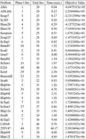
TABLE8.1.3. Algorithm I test statistics (IBM 3090) — NETLIB test problems (minimum degree ordering heuristic in Algorithm I)
Problem Phase I Itrs Total Itrs Time (secs.) Objective Value
Afiro 1 20 0.04 -4.6475315e+02
ADLittle 1 24 0.12 2.2549496e+05
Scagr7 3 25 0.17 -2.3313898e+06
Sc205 4 29 0.28 -5.2202061e+01
Share2b 4 28 0.29 -4.1573224e+02
Share1b 7 39 0.58 -7.6589319e+04
Scorpion 5 25 0.51 1.8781248e+03
Scagr25 3 28 0.69 -1.4753433e+07
ScTap1 6 34 0.85 1.4122488e+03
BrandY 38 38 1.52 1.5185099e+03
Scsd1 2 19 0.41 8.6666666e+00
Israela 8 38 4.00 -8.9664483e+05
BandM 7 33 1.54 -1.5862802e+02
Scfxm1 33 33 1.97 1.8416759e+04
E226 40 40 1.56 -1.8751929e+01
Scrs8 39 39 2.30 9.0429695e+02
Beaconfd 23 23 0.69 3.3592486e+04
Scsd6 2 22 0.83 5.0500000e+01
Ship04s 5 31 1.26 1.7987145e+06
Scfxm2 38 38 4.38 3.6660261e+04
Ship04l 5 31 2.31 1.7933245e+06
Ship08s 5 34 1.58 1.9200982e+06
ScTap2 7 33 6.71 1.7248068e+03
Scfxm3 37 37 6.66 5.4901254e+04
Ship12s 4 35 1.91 1.4892361e+06
Scsd8 2 24 1.68 9.0500000e+02
ScTap3 7 36 9.44 1.4240000e+03
CzProb 3 46 9.76 2.1851927e+06
25FV47 44 55 46.17 5.5018494e+03
Ship08l 5 34 4.00 1.9090552e+06
Ship12l 5 34 4.89 1.4701879e+06
aThe conjugate gradient algorithm was triggered when running this test problem.
• Iterations for Algorithm I vary from 19 to 55 (see Tables 8.1.3 and 8.1.4), growing slowly with problem size.
TABLE8.1.4. Algorithm I test statistics (IBM 3090) — NETLIB test problems (minimum local fill-in ordering heuristic)
Problem Phase I Itrs Total Itrs Time (secs.) Objective Value
Afiro 1 20 0.05 -4.6475315e+02
ADLittle 1 24 0.13 2.2549496e+05
Scagr7 3 24 0.18 -2.3313898e+06
Sc205 4 28 0.26 -5.2202061e+01
Share2b 4 29 0.32 -4.1573224e+02
Share1b 7 38 0.47 -7.6589319e+04
Scorpion 5 24 0.49 1.8781248e+03
Scagr25 3 29 0.70 -1.4753433e+07
ScTap1 6 33 0.80 1.4122488e+03
BrandY 38 38 1.49 1.5185099e+03
Scsd1 2 19 0.44 8.6666666e+00
Israela 8 37 4.01 -8.9664483e+05
BandM 7 30 1.26 -1.5862802e+02
Scfxm1 33 33 1.66 1.8416759e+04
E226 34 34 1.58 -1.8751929e+01
Scrs8 39 39 2.28 9.0429695e+02
Beaconfd 23 23 0.62 3.3592486e+04
Scsd6 2 22 0.84 5.0500000e+01
Ship04s 5 30 1.01 1.7987145e+06
Scfxm2 38 39 3.83 3.6660261e+04
Ship04l 5 28 1.39 1.7933245e+06
Ship08s 5 32 1.35 1.9200982e+06
ScTap2 7 34 5.52 1.7248068e+03
Scfxm3 37 40 5.87 5.4901254e+04
Ship12s 4 35 1.75 1.4892361e+06
Scsd8 2 23 1.82 9.0500000e+02
ScTap3 7 36 7.78 1.4240000e+03
CzProb 3 52 3.64 2.1851927e+06
25FV47 44 54 31.70 5.5018494e+03
Ship08l 5 31 2.44 1.9090552e+06
Ship12l 5 32 3.43 1.4701879e+06
aThe conjugate gradient algorithm was triggered when running this test problem.
TABLE 8.1.5. Algorithm II test statistics (IBM 3081-K) — NETLIB test problems (minimum degree ordering heuristic in Algorithm II)
Problema Phase I Itrs Total Itrs Time (secs.) Objective Value
Afiro 1 15 0.08 -4.6475315e+02
ADLittle 1 18 0.27 2.2549496e+05
Scagr7 3 19 0.43 -2.3313898e+06
Sc205 3 20 0.66 -5.2202061e+01
Share2b 4 21 0.69 -4.1573224e+02
Share1b 5 33 1.47 -7.6589319e+04
Scorpion 4 19 1.22 1.8781248e+03
Scagr25 3 21 1.71 -1.4753433e+07
ScTap1 5 23 2.00 1.4122488e+03
BrandY 24 24 2.79 1.5185099e+03
Scsd1 2 16 1.10 8.6666666e+00
Israel 6 29 8.22 -8.9664483e+05
BandM 4 24 3.46 -1.5862802e+02
Scfxm1 30 30 4.94 1.8416759e+04
E226 30 30 3.54 -1.8751929e+01
Scrs8 29 29 5.07 9.0429695e+02
Beaconfd 17 17 1.51 3.3592486e+04
Scsd6 2 18 2.13 5.0500000e+01
Ship04s 4 22 2.85 1.7987145e+06
Scfxm2 29 29 9.28 3.6660261e+04
Ship04l 4 21 4.71 1.7933245e+06
Ship08s 4 21 3.30 1.9200982e+06
ScTap2 5 25 13.55 1.7248068e+03
Scfxm3 30 30 14.25 5.4901254e+04
Ship12s 3 23 4.17 1.4892361e+06
Scsd8 2 18 4.22 9.0500000e+02
ScTap3 6 27 19.59 1.4240000e+03
CzProb 3 35 14.33 2.1851927e+06
Ship08l 4 23 8.12 1.9090552e+06
Ship12l 4 23 10.07 1.4701879e+06
aProblem 25FV47 was not solved with Algorithm II, as its current implementation does not incorporate a dense
window data structure (Adler et al. 1989) necessary to solve this problem under a 4 Mbytes memory limit.
TABLE8.1.6. Comparison of run times (IBM 3090) — NETLIB Test Problems (minimum local fill-in ordering heuristic)
Problem MINOS Alg-I Alg-IIa MINOS Alg-I MINOS Alg-II
Time Time Time Time Ratio Time Ratio
(secs.) (secs.) (secs.)
Afiro 0.01 0.05 0.08 0.2 0.5
ADLittle 0.23 0.13 0.27 1.8 1.7
Scagr7 0.29 0.18 0.43 1.6 1.2
Sc205 0.45 0.26 0.66 1.7 1.6
Share2b 0.26 0.32 0.69 0.8 0.9
Share1b 1.27 0.47 1.47 2.7 1.8
Scorpion 1.06 0.49 1.22 2.2 2.1
Scagr25 4.54 0.70 1.71 6.5 6.1
ScTap1 1.98 0.80 2.00 2.5 1.7
BrandY 1.34 1.49 2.79 0.9 1.1
Scsd1 1.02 0.44 1.10 2.3 2.2
Israel 1.54 4.01 8.22 0.4 0.4
BandM 2.54 1.26 3.46 2.0 1.9
Scfxm1 2.04 1.66 4.94 1.2 1.0
E226 3.68 1.58 3.54 2.3 1.7
Scrs8 5.64 2.28 5.07 2.5 1.9
Beaconfd 0.18 0.62 1.51 0.3 0.3
Scsd6 2.69 0.84 2.13 3.2 3.9
Ship04s 3.54 1.01 2.85 3.5 2.1
Scfxm2 8.18 3.83 9.28 2.1 1.8
Ship04l 7.18 1.39 4.71 5.2 2.5
Ship08s 9.16 1.35 3.30 6.8 4.6
ScTap2 22.02 5.52 13.52 4.0 2.8
Scfxm3 19.31 5.87 14.25 3.3 2.5
Ship12s 12.78 1.75 4.17 7.3 5.6
Scsd8 14.53 1.82 4.22 8.0 7.7
ScTap3 32.87 7.78 18.95 4.2 3.0
CzProb 39.08 3.64 14.33 10.7 4.3
25FV47 217.67 31.70 NA 6.9 NA
Ship08l 14.72 2.44 8.12 6.0 4.0
Ship12l 26.10 3.43 10.07 7.6 5.5
aIBM 3081-K CPU times and minimum degree ordering heuristic in Algorithm II.
TABLE 8.1.7. Iteration, time per iteration and total time ratios for NETLIB subgroups (IBM 3090) (minimum local fill-in ordering heuris-tic)
Problem Rows Columns MINOS Alg-I MINOS Alg-I MINOS Alg-I Iter. Ratio Time/Iter. Ratio Time Ratio
Scsd1 77 760 13.7 0.169 2.32
Scsd6 147 1350 26.2 0.122 3.20
Scsd8 397 2750 69.1 0.115 7.98
Scfxm1 330 600 13.2 0.093 1.23
Scfxm2 660 1200 20.3 0.105 2.14
Scfxm3 990 1800 29.9 0.110 3.29
ScTap1 300 660 9.2 0.268 2.47
ScTap2 1090 2500 33.0 0.121 3.99
ScTap3 1480 3340 35.4 0.119 4.22
Ship04s 402 1506 10.3 0.340 3.50
Ship08s 778 2467 20.5 0.330 6.79
Ship12s 1151 2869 20.5 0.356 7.30
Ship04l 402 2166 21.2 0.244 5.17
Ship08l 778 4363 30.9 0.195 6.03
Ship12l 1151 5533 39.6 0.192 7.61
Thus, relative to simplex based codes, Algorithm I becomes increasingly faster as the problems get larger.
• The optimal objective values reported in Table 8.1.3 are accurate within 6 and 8 digits if compared to the values reported in (Gay 1985). The primal solution computed at termination was accurate in most cases with the exception of problems CzProb and 25FV47 (see Table 8.1.8). The primal-dual relation presented for problem Israel are based on an implementation using direct factorization to compute the search direc-tions at each iteration.
• All of the above considerations made for Algorithm I are valid for Algorithm II. Fur-thermore, Algorithm II requires on average 26% less iterations to converge to 8 digit accuracy than Algorithm I. However, this does not translate into any significant gain in solution time, since the extra work per iteration in the current implementation off-sets the savings in the number of iterations. We believe that by refining the extra com-putation, further reduction in work per iteration in Algorithm II is possible, leading to a faster implementation.
TABLE 8.1.8. Primal dual relations for Algorithm I (IBM 3090) — NETLIB test problems
Problem Relative Max. Normal. Min. Normal. Max. Normal. Duality Gap Primal Infeas. Primal Entry Complem. Viol.
Afiro 3.56e-09 1.58e-15 -5.76e-24 7.99e-12
ADLittle 3.69e-09 1.05e-11 -9.67e-22 3.06e-12
Scagr7 3.16e-09 2.31e-10 -4.02e-20 6.27e-13
Sc205 2.41e-09 2.23e-13 -2.61e-20 2.73e-13
Share2b 6.83e-11 2.09e-12 -1.06e-16 1.84e-12
Share1b 3.33e-09 3.26e-09 -1.73e-21 8.31e-15
Scorpion 2.84e-09 5.27e-12 -6.07e-13 1.14e-12
Scagr25 1.06e-08 1.32e-10 -9.73e-23 4.50e-13
ScTap1 2.25e-09 1.41e-13 -2.96e-21 9.40e-14
BrandY 1.34e-09 4.00e-06 -6.91e-04 5.43e-14
Scsd1 3.31e-09 4.90e-13 -1.05e-14 1.17e-11
Israel 1.22e-09 5.46e-12 -5.38e-24 1.11e-15
BandM 1.06e-08 2.12e-09 -1.28e-16 1.76e-13
Scfxm1 1.20e-07 7.29e-07 -8.78e-19 5.03e-13
E226 4.10e-09 3.36e-07 -5.94e-05 1.51e-13
Scrs8 1.70e-09 7.28e-06 -1.67e-09 3.55e-15
Beaconfd 1.44e-09 1.42e-06 -6.48e-06 9.23e-12
Scsd6 9.81e-10 4.30e-10 -1.61e-16 7.15e-13
Ship04s 8.34e-09 2.41e-09 -4.95e-14 1.45e-11
Scfxm2 1.54e-08 5.99e-10 -1.78e-19 2.19e-13
Ship04l 2.15e-09 2.25e-11 -1.75e-16 3.01e-12
Ship08s 1.56e-09 1.09e-11 -4.24e-18 1.40e-12
ScTap2 1.06e-08 9.57e-15 -6.09e-20 2.00e-13
Scfxm3 9.29e-09 4.11e-10 -5.37e-20 8.30e-14
Ship12s 8.16e-09 1.78e-09 -1.74e-15 2.96e-12
Scsd8 4.26e-09 1.35e-14 -4.67e-21 6.15e-13
ScTap3 1.73e-09 1.08e-14 -1.01e-20 4.23e-14
CzProb 1.60e-09 1.11e-05 -1.02e-19 1.19e-14
25FV47 1.22e-08 5.43e-03 -3.17e-06 7.54e-15
Ship08l 4.11e-10 1.02e-09 -3.05e-18 4.29e-13
Ship12l 1.27e-09 9.38e-10 -2.19e-17 2.83e-13
iteration the accuracy of the primal solution for problem Israel was similar to those reported for the other problems.
TABLE8.2.1. Multi-commodity network flow test problems statistics
Problem Nodes Commodities LP Rows LP Columns Nonz(A)
MUL031 300 1 1406 2606 5212
MUL041 400 1 1888 2488 6976
MUL051 500 1 2360 4360 8720
MUL061 600 1 2853 5253 10506
MUL043 400 3 2008 4027 9670
MUL053 500 3 2489 4949 11876
MUL063 600 3 2981 5882 14126
MUL035 300 5 2081 4436 11196
MUL045 400 5 2793 5948 15068
MUL055 500 5 3477 7637 19182
MUL065 600 5 4135 8800 22140
of the linear programming algorithm, the total savings more than offsets the extra processing in the ordering procedure. The sum of the solution times (including re-ordering) for all test problems was reduced from 119.10 seconds to 89.11 seconds with minimal local fill-in, corresponding to a 25% reduction. Solution times for Al-gorithm I with minimal local fill-in were faster on 21 out the 31 test problems and on 11 of the 12 problems having more than 5000 nonzero elements (see deCarvalho (1987)).
8.2. Multi-Commodity Network Flow Problems. In this section, we report on 11 multi-commodity network flow problems generated with MNETGN (Ali & Kennington 1977), a random multi-commodity network flow problem generator. MNETGN generates a ran-dom network structure based on the number of arcs and nodes supplied by the user. Addi-tional user specifications include the number of commodities and the ranges of arc costs and capacities. Table 8.2.1 displays the basic data for this set of test problems. We generated multi-commodity network flow problem by varying the number of nodes and commodities and keeping the same relative number of arcs. The test problems were solved with Algo-rithm I, MINOS and MCNF85 (Kennington 1979), a special purpose simplex code for multi-commodity network flow problems. Algorithm I used the minimum degree ordering heuristic and the same parameter selection described in Section 8.1. All runs were carried out on an IBM 3090 Tables 8.2.2–8.2.4 and Figure 8.2.1 present the statistics for these runs.
We list below a few observations on the test results reported on this section.
TABLE8.2.2. Algorithm I test statistics (IBM 3090) — Multicommod-ity Networks (minimum degree ordering heuristic in Algorithm I)
Problem Phase I iter. Total iter. Time (secs.)
MUL031 3 33 6.51
MUL041 2 28 11.79
MUL051 2 33 23.07
MUL061 2 31 30.96
MUL043 2 27 24.27
MUL053 2 30 47.84
MUL063 2 28 58.57
MUL035 2 30 55.81
MUL045 2 30 104.34
MUL055 2 36 204.71
MUL065 2 35 309.50
TABLE8.2.3. MINOS 4.0 test statistics (IBM 3090) — Multicommod-ity Networks)
Problem Phase I Itrs Total Itrs Time (secs.)
MUL031 362 940 12.73
MUL041 457 1351 24.11
MUL051 620 1807 40.65
MUL061 817 2358 63.88
MUL043 2498 5926 196.38
MUL053 3366 8115 345.69
MUL063 4855 12286 677.31
MUL035 2930 6691 249.71
MUL045 4611 12193 666.58
MUL055 5919 15238 1045.67
MUL065 7693 21915 1885.34
• It is interesting to note that despite being a general purpose implementation, rithm I performed comparably to MCNF85. A tailored implementation of Algo-rithm I (e.g. with integer operations and specialized Gaussian elimination) could im-prove on current results. Furthermore, the trend in the data (Table 8. 2.6) suggests that for larger problems Algorithm I could outperform MCNF85.
• The objective values for the solutions obtained with our implementation of Algo-rithm I achieved 8 digits accuracy when compared to the values obtained by MINOS. Also a feasible primal solution was recovered at the end of the algorithm with the same degree of accuracy.
TABLE 8.2.4. MCNF85 test statistics (IBM 3090) — Multi-commodity networks
Problem Total iter. Time (sec.)
MUL031 931 7.42
MUL041 1087 11.39
MUL051 1892 24.87
MUL061 3082 53.45
MUL043 4983 45.23
MUL053 5158 55.60
MUL063 16983 243.35
MUL035 4132 34.64
MUL045 10558 111.30
MUL055 8862 121.66
MUL065 16624 260.44
TABLE 8.2.5. MINOS /Algorithm I performance ratios — Multicom-modity Networks (minimum local fill-in ordering heuristic)
Problem Nodes Commodities MINOS /Alg-I MINOS /Alg-I MINOS /Alg-I iter. ratio time/iter ratio time ratio
MUL031 300 1 28.5 0.069 1.96
MUL041 400 1 48.3 0.042 2.04
MUL051 500 1 54.8 0.032 1.76
MUL061 600 1 76.1 0.027 2.06
MUL043 400 3 219.5 0.037 8.09
MUL053 500 3 270.5 0.027 7.23
MUL063 600 3 438.8 0.026 11.56
MUL035 300 5 223.0 0.020 4.47
MUL045 400 5 406.4 0.016 6.39
MUL055 500 5 423.3 0.012 5.11
MUL065 600 5 626.1 0.010 6.09
increasing sizes were generated. Under the framework of FORPLAN a forest is divided into management units called analysis areas, each comprising a collection of acres from across the forest, sharing similar silvicultural and economic characteristics. Our test prob-lems were created by successively increasing the number of analysis areas, resulting in models that represent subsets of the original forest. FORPLAN is widely used through-out the United States national forest system, yielding very large linear programs that pose a considerable challenge to linear programming codes. Table 8.3.1 presents the basic sta-tistics of this family of test problems.
TABLE8.2.6. MCNF85 /Algorithm I performance ratios — Multicom-modity Networks (minimum local fill-in ordering heuristic)
Problem Nodes Commodities MCNF85 /Alg-I MCNF85 /Alg-I MCNF85 /Alg-I iter. ratio time/iter ratio time ratio
MUL031 300 1 28.2 0.0404 1.14
MUL041 400 1 38.8 0.0249 0.97
MUL051 500 1 57.3 0.0188 1.08
MUL061 600 1 99.4 0.0174 1.73
MUL043 400 3 184.6 0.0101 1.86
MUL053 500 3 171.9 0.0068 1.16
MUL063 600 3 606.5 0.0069 4.15
MUL035 300 5 137.7 0.0045 0.62
MUL045 400 5 351.9 0.0030 1.07
MUL055 500 5 246.2 0.0024 0.59
MUL065 600 5 475.0 0.0018 0.84
0 200 400 600 800 1000 1200 1400 1600 1800
6000 8000 10000 12000 14000 16000 18000 20000 22000 CPU Time
(seconds)
Number of Nonzero elements MINOS b
b b
b b
b b
b
b b
b
b
Algorithm I r
r r
r r
r r
r
r r
r
r
MCNF85 ×
× × × × × × ×
×
× ×
×
FIGURE 8.2.1. MINOS 4.0, MCNF85 and Algorithm I (CPU times, IBM 3090) — Multicommodity Flows (minimum degree ordering heuristic in Algorithm I)
TABLE8.3.1. Timber harvest scheduling test problems statistics
Problem LP Rows LP Columns Nonz(A)
FPK010 55 744 6021
FPK040 58 973 8168
FPK050 64 1502 12765
FPK080 76 2486 21617
FPK100 87 3357 30104
FPK150 109 4993 43774
FPK200 130 6667 59057
FPK300 177 9805 86573
FPK400 220 12570 109697
FPK500 266 16958 149553
FPK600 316 19991 176346
test problems, the manipulation of the PARTIAL PRICE parameter, which sets the number of segments in the partition, can impact the performance of MINOS enormously. Conse-quently, we compare MINOS with Algorithm I using the following pricing strategies:
• Total Pricing Strategy: Each pricing operation examines the total set of variables.
• Default Pricing Strategy: Sets the PARTIAL PRICE parameter to half of the ratio of number of columns to number of rows.
• Improved Pricing Strategy: Sets the PARTIAL PRICE parameter to eight times the ratio of number of columns to number of rows. We arrived at this strategy after ex-tensive testing with some of the test problems.
Tables 8.3.2–8.3.8 display the results of running the test problems with Algorithm I and MINOS under the three pricing strategies. Figure 8.3.1 illustrates graphically the compu-tational performance of the algorithms. All run were carried out on an IBM 3090 with same characteristics as in tests reported in Section 8.1. We use minimum degree ordering heuristic in Algorithm I.
We close this section with a few observations on the results of the runs with the timber harvest scheduling problems.
• The theoretical worst case analysis of Karmarkar’s algorithm (Karmarkar 1984) sug-gests that the number of iterations should grow linearly with the largest dimension of the coefficient matrix. This behavior is not is not confirmed for the variants of the algorithm described here. In this set of test problems, with number of columns rang-ing from 744 to 19991, the number of iterations until convergence grows sublinearly, varying from 38 to 71, consistent with our earlier observation that the number of it-erations grows slowly with problem size.
TABLE 8.3.2. Algorithm I test statistics — Timber harvest scheduling problems (minimum degree ordering heuristic)
Problem Phase I iter. Total iter. Time (sec.)
FPK010 4 38 0.85
FPK040 4 40 1.10
FPK050 4 41 1.64
FPK080 5 49 2.95
FPK100 5 49 4.27
FPK150 5 49 6.47
FPK200 5 56 9.60
FPK300 6 52 14.99
FPK400 5 43 24.81
FPK500 6 67 34.11
FPK600 6 71 43.80
TABLE8.3.3. MINOS 4.0 test statistics (total pricing) — Timber har-vest scheduling problems
Problem Partial Phase I Total Time Pricing iter. iter. (sec.)
FPK010 1 449 534 3.52
FPK040 1 579 736 5.63
FPK050 1 688 878 9.87
FPK080 1 1318 1574 28.81
FPK100 1 1521 1827 43.18
FPK150 1 2350 2768 93.77
FPK200 1 2867 3446 154.78
FPK300 1 4570 5407 351.82
FPK400 1 5375 7300 600.75
FPK500 1 7322 10156 1112.68
FPK600 1 3488 12009 1582.80
out computational experiments involving the simplex method, as varying a single pa-rameter among different runs of MINOS the execution time for the two largest test problems is reduced by a factor of over 100.
• Our implementation of Algorithm I is faster than the most straightforward version of MINOS by a wide margin (see Table 8.3.3 and Figure 8.3.1) and is up to 2.8 times faster for runs using the default pricing strategy . However, MINOS runs up to 3 times faster when using the improved pricing strategy in a pricing strategy obtained after extensive experimentation.
TABLE 8.3.4. MINOS (Total Pricing) Algorithm I performance ra-tios — Timber harvest scheduling problems (minimum degree ordering heuristic in Algorithm I)
Problem Partial MINOS Alg-I MINOS Alg-I MINOS Alg-I Pricing iter. ratio time/iter. ratio time ratio
FPK010 1 14.05 0.2947 4.14
FPK040 1 18.40 0.2782 5.12
FPK050 1 21.41 0.2810 6.02
FPK080 1 32.12 0.3040 9.77
FPK100 1 37.29 0.2712 10.11
FPK150 1 56.49 0.2566 14.49
FPK200 1 61.54 0.2620 16.12
FPK300 1 103.98 0.2257 23.47
FPK400 1 169.77 0.1426 24.21
FPK500 1 151.58 0.2152 32.62
FPK600 1 169.14 0.2137 36.14
TABLE 8.3.5. MINOS 4.0 test statistics (default pricing) — Timber harvest scheduling problems
Problem Partial Phase I Total Time pricing iter. iter. (sec.)
FPK010 1 449 534 3.52
FPK040 1 579 736 5.63
FPK050 11 724 902 2.74
FPK080 16 973 1259 4.48
FPK100 19 1460 1832 7.39
FPK150 22 1860 2352 11.37
FPK200 25 2707 3369 17.94
FPK300 27 3244 4370 29.74
FPK400 28 4536 6035 49.13
FPK500 31 6934 9732 93.89
FPK600 31 3421 11364 123.62
Also a feasible primal solution was recovered at the end of the algorithm with the same degree of accuracy.
8.4. Interpretation of Computational Experiments. We make the following interpreta-tion of the results of the computainterpreta-tional experiments.
TABLE 8.3.6. MINOS (Default Pricing)/Algorithm I performance ra-tios — Timber harvest scheduling problems (minimum degree ordering heuristic in Algorithm I)
Problem Partial MINOS Alg-I MINOS Alg-I MINOS Alg-I pricing iter. ratio time/iter. Ratio time ratio
FPK010 1 14.05 0.2947 4.14
FPK040 1 18.40 0.2782 5.12
FPK050 11 22.00 0.0759 1.67
FPK080 16 25.69 0.0591 1.52
FPK100 19 37.39 0.0463 1.73
FPK150 22 48.00 0.0366 1.76
FPK200 25 60.16 0.0311 1.87
FPK300 27 84.04 0.0236 1.98
FPK400 28 140.35 0.0141 1.98
FPK500 31 145.25 0.0190 2.75
FPK600 31 160.06 0.0176 2.82
TABLE8.3.7. MINOS 4.0 test statistics (improved pricing) — Timber harvest scheduling problems
Problem Partial Phase I Total Time pricing iter. iter. (sec.)
FPK010 104 48 1738 2.54
FPK040 128 137 812 1.52
FPK050 160 79 478 1.04
FPK080 184 113 333 1.13
FPK100 360 77 379 1.89
FPK150 480 105 542 2.96
FPK200 480 174 558 3.96
FPK300 440 455 924 6.61
FPK400 440 461 1049 8.41
FPK500 480 387 843 9.30
FPK600 480 729 1329 13.26
• The selection of an initial interior solution as described in Section 6 plays a signifi-cant role in the fast convergence observed in all test problems. In this procedure, we attempt to start the algorithm far from faces of the feasible polyhedral set, avoiding the difficulties described by Megiddo & Shub (1989).
TABLE8.3.8. MINOS (improved pricing)/Algorithm I performance ra-tios — Timber harvest scheduling problems (minimum degree ordering heuristic in Algorithm I)
Problem Partial MINOS Alg-I MINOS Alg-I MINOS Alg-I pricing iter. ratio time/iter. ratio time ratio
FPK010 104 45.74 0.0653 2.99
FPK040 128 20.30 0.0681 1.38
FPK050 160 11.66 0.0544 0.63
FPK080 184 6.80 0.0564 0.38
FPK100 360 7.73 0.0572 0.44
FPK150 480 11.06 0.0414 0.46
FPK200 480 9.96 0.0414 0.41
FPK300 440 17.77 0.0248 0.44
FPK400 440 24.40 0.0139 0.34
FPK500 480 12.58 0.0217 0.27
FPK600 480 18.72 0.0162 0.30
0 200 400 600 800 1000 1200 1400 1600
0 20000 40000 60000 80000 100000 120000 140000 160000 180000 CPU Time
(seconds)
Number of Nonzero elements Algorithm I r
rr r r r r
r r
r
r
r
MINOS(Total pricing) b
bb b
b b
b b
b
b
b
b
MINOS(Default pricing) ×
××× × × × × × × ×
× MINOS(Improved pricing) ⋆
⋆⋆ ⋆ ⋆ ⋆ ⋆ ⋆ ⋆ ⋆ ⋆ ⋆
FIGURE 8.3.1. MINOS 4.0 and Algorithm I (CPU times, IBM 3090) — Timber harvest problems (minimum degree ordering heuristic in Al-gorithm I)
• Usingδ=0.1 in updating the ATD−2
v A matrix, Algorithm I obtained savings of over
10% in execution times, when compared to full updating, without degradation of the method’s numerical stability.
• Algorithm I is sensitive to the density of the ATD−v2A matrix. Hence, besides being sparse, the AT matrix should have a small number of dense columns. Maintaining
this matrix sparse is essential to the algorithm.
9. CONCLUSION ANDEXTENSIONS
The computational results presented in this paper illustrate the potential of interior point methods for linear programming. While the implementation described here was developed in a short period of time, it still outperforms MINOS 4.0 on the majority of problems tested. For test problems from the NETLIB collection, solution time speed-ups 6 or higher are observed on most of mid-sized problems, and increase with problem size. Seven and eight digit accuracy in the objective function value was achieved on all test problems, except for problems ScTap1, CzProb and 25FV47 . An optimal complementary primal-dual pair was obtained for all test problems with exception of CzProb and 25FV47 . Numerical difficulties with the LU towards the end of the algorithm account for these inaccuracies.
Among the test problems is a set of multi-commodity network flow problems. The inte-rior algorithm was clearly supeinte-rior to MINOS and was also competitive with a specialized simplex algorithm, MCNF85. For the set of timber harvest scheduling problems, linear programs with significantly more variables than constraints, the number of iterations re-quired by Algorithm I grows slowly with the number of variables. However, specialized pricing strategies make the simplex method a better tool for solving this type of linear pro-gramming problems.
The implementations of interior point algorithms described in this paper are still pre-liminary. Since many improvements are still possible this approach seems promising as a general purpose solver for large real-world linear programming problem s. Of the several extensions planned to our implementation, some are immediately required:
• Implicit treatment of upper and lower bounds on the variables.
• Feasibility adjustment of the tentative primal solution computed at the end of the al-gorithm.
Other extensions planned are:
• Preprocessor for increasing sparsity of input matrices.
• Higher order approximations to the solution of system differential equation 3.9–3.11.
• Optimal basis identification for early termination.
• Bi-directional search for determining the step direction.
• Develop primal and primal-dual implementations.
• Include steps in potential function gradient direction.
• Implementations for special LP structures, e.g. network flows and GUB.
• Implementation for parallel computer architectures.
ACKNOWLEDGMENT