Biomechanical Systems Techniques and Applications Musculoskeletal Models & Techniques pdf

Cornelius Leondes

E D I T E D BY

Biomechanical Systems

Techniques

and

Applications

V O L U M E I I I

Musculoskeletal

Models

and

Techniques

This book contains information obtained from authentic and highly regarded sources. Reprinted material is quoted with permission, and sources are indicated. A wide variety of references are listed. Reasonable efforts have been made to publish reliable data and information, but the author and the publisher cannot assume responsibility for the validity of all materials or for the consequences of their use.

Neither this book nor any part may be reproduced or transmitted in any form or by any means, electronic or mechanical, including photocopying, microfilming, and recording, or by any information storage or retrieval system, without prior permission in writing from the publisher.

All rights reserved. Authorization to photocopy items for internal or personal use, or the personal or internal use of specific clients, may be granted by CRC Press LLC, provided that $.50 per page photocopied is paid directly to Copyright Clearance Center, 222 Rosewood Drive, Danvers, MA 01923 USA. The fee code for users of the Transactional Reporting Service is ISBN 0-8493-9048-6/00/$0.00+$.50. The fee is subject to change without notice. For organizations that have been granted a photocopy license by the CCC, a separate system of payment has been arranged.

The consent of CRC Press LLC does not extend to copying for general distribution, for promotion, for creating new works, or for resale. Specific permission must be obtained in writing from CRC Press LLC for such copying.

Direct all inquiries to CRC Press LLC, 2000 N.W. Corporate Blvd., Boca Raton, Florida 33431.

Trademark Notice: Product or corporate names may be trademarks or registered trademarks, and are used only for identification and explanation, without intent to infringe.

© 2000 by CRC Press LLC

No claim to original U.S. Government works International Standard Book Number 0-8493-9048-6 Printed in the United States of America 1 2 3 4 5 6 7 8 9 0

Printed on acid-free paper

Library of Congress Cataloging-in-Publication Data

Preface

Because of rapid developments in computer technology and computational techniques, advances in a wide spectrum of technologies, and other advances coupled with cross-disciplinary pursuits between technology and its applications to human body processes, the field of biomechanics continues to evolve. Many areas of significant progress can be noted. These include dynamics of musculoskeletal systems, mechanics of hard and soft tissues, mechanics of bone remodeling, mechanics of implant-tissue interfaces, cardiovascular and respiratory biomechanics, mechanics of blood and air flow, flow-prosthesis interfaces, mechanics of impact, dynamics of man–machine interaction, and more.

Needless to say, the great breadth and significance of the field on the international scene require several volumes for an adequate treatment. This is the third in a set of four volumes, and it treats the area of musculoskeletal models and techniques.

The four volumes constitute an integrated set that can nevertheless be utilized as individual volumes. The titles for each volume are

Computer Techniques and Computational Methods in Biomechanics Cardiovascular Techniques

Musculoskeletal Models and Techniques

Biofluid Methods in Vascular and Pulmonary Systems

The Editor

Contents

1

Three-Dimensional Dynamic Anatomical Modeling of the

Human Knee Joint

Mohamed Samir Hefzy and

Eihab Muhammed Abdel-Rahman

2

Techniques and Applications of Adaptive Bone Remodeling Concepts

Nicole M. Grosland, Vijay K. Goel, and Roderic S. Lakes

3

Techniques in the Dynamic Modeling of Human Joints with a

Special Application to the Human Knee

A.E. Engin

4

Techniques and Applications of Scanning Acoustic Microscopy in

Bone Remodeling Studies

Mark C. Zimmerman, Robert D. Harten, Jr.,

Sheu-Jane Shieh, Alain Meunier, and J. Lawrence Katz

5

Techniques and Applications for Strain Measurements of Skeletal

Muscle

Chris Van Ee and Barry S. Myers

6

A Review of the Technologies and Methodologies Used to

Quantify Muscle-Tendon Structure and Function

David Hawkins

1

Three-Dimensional

Dynamic Anatomical

Modeling of the

Human Knee Joint

1.1 Background

Biomechanical Systems • Physical Knee Models •

Phenomenological Mathematical Knee Models • Anatomically Based Mathematical Knee Models

1.2 Three-Dimensional Dynamic Modeling of the

Tibio-Femoral Joint: Model Formulation

Kinematic Analysis • Contact and Geometric Compatibility Conditions • Ligamentous Forces • Contact Forces • Equations of Motion

1.3 Solution Algorithm

DAE Solvers • Load Vector and Stiffness Matrix

1.4 Model Calculations

1.5 Discussion

Varus-Valgus Rotation • Tibial Rotation • Femoral and Tibial Contact Pathways • Velocity of the Tibia • Magnitude of the Tibio-Femoral Contact Forces • Ligamentous Forces

1.6 Conclusions

1.7 Future Work

Three-dimensional dynamic anatomical modeling of the human musculo-skeletal joints is a versatile tool for the study of the internal forces in these joints and their behavior under different loading conditions following ligamentous injuries and different reconstruction procedures. This chapter describes the three-dimensional dynamic response of the tibio-femoral joint when subjected to sudden external pulsing loads utilizing an anatomical dynamic knee model. The model consists of two body segments in contact (the femur and the tibia) executing a general three-dimensional dynamic motion within the constraints of the ligamentous structures. Each of the articular surfaces at the tibio-femoral joint is represented by a separate mathematical function. The joint ligaments are modeled as nonlinear elastic springs. The six-degrees-of-freedom joint motions are characterized using six kinematic parameters and ligamentous forces are expressed in terms of these six parameters. In this formulation, all the coordinates of the ligamentous attachment points are dependent variables which allow one to easily introduce more liga-ments and/or split each ligament into several fiber bundles. Model equations consist of nonlinear second order ordinary differential equations coupled with nonlinear algebraic constraints. An algorithm was developed to solve this differential-algebraic equation (DAE) system by employing a DAE solver, namely, the Differential Algebraic System Solver (DASSL) developed at Lawrence Livermore National Laboratory. Mohamed Samir Hefzy

University of Toledo

Eihab Muhammed Abdel-Rahman

Model calculations show that as the knee was flexed from 15 to 90°, it underwent internal tibial rotation. However, in the first 15° of knee flexion, this trend was reversed: the tibia rotated internally as the knee was extended from 15° to full extension. This indicates that the screw-home mechanism that calls for external rotation in the final stages of knee extension was not predicted by this model. This finding is important since it is in agreement with the emerging thinking about the need to re-evaluate this mechanism.

It was also found that increasing the pulse amplitude and duration of the applied load caused a decrease in the magnitude of the tibio-femoral contact force at a given flexion angle. These results suggest that increasing load level caused a decrease in joint stiffness. On the other hand, increasing pulse amplitude did not change the load sharing relations between the different ligamentous structures. This was expected since the forces in a ligament depend on its length which is a function of the relative position of the tibia with respect to the femur.

Reciprocal load patterns were found in the anterior and posterior fibers of both anterior and posterior cruciate ligaments, (ACL) and (PCL), respectively. The anterior fibers of the ACL were slack at full extension and tightened progressively as the knee was flexed, reaching a maximum at 90° of knee flexion. The posterior fibers of the ACL were most taut at full extension; this tension decreased until it vanished around 75° of knee flexion. The forces in the anterior fibers of the PCL increased from zero at full extension to a maximum around 60° of knee flexion, and then decreased to 90° of knee flexion. On the other hand, the posterior fibers of the PCL were found to carry lower loads over a small range of motion; these forces were maximum at full extension and reached zero around 10° of knee flexion. These results suggest that regaining stability of an ACL deficient knee would require the reconstruction of both the anterior and posterior fibers of the ACL. On the other hand, these data suggest that it might be sufficient to reconstruct the anterior fibers of the PCL to regain stability of a PCL deficient knee.

1.1 Background

Biomechanical Systems

Biomechanics is the study of the structure and function of biological systems by the means of the methods of mechanics.63 _{Biomechanics thus provides the means to study and analyze the behaviors of the different}

biological systems as well as their components. Models have emerged as necessary and effective tools to be employed in the analysis of these biomechanical systems.

In general, employing models in system analysis requires two prerequisites: a clear objective identifying the aims of the study, and an explicit specification of the assumptions to be made. A system mainly depends upon what it is being used to determine, e.g., joint stiffness or individual ligament lengths and forces. The system is thus identified according to the aim of the study. Assumptions are then introduced in order to simplify the system and construct the model. These assumptions also depend on the aim of the study. For example, if the intent is to determine the failure modes of a tendon, it is not reasonable to model the action of a muscle as a single force applied to the muscle’s attachement point. On the other hand, this assumption is appropriate if it is desired to determine the effect of a tendon transfer on gait. After the system has been defined and simplified, the modeling process continues by identifying system variables and parameters. The parameters of a system characterize its components while the variables describe its response. The variables of a system are also referred to as the quantities being determined.

Modeling activities include the development of physical models and/or mathematical models. The mechanical responses of physical models are determined by conducting experimental studies on fabri-cated structures to simulate some aspect of the real system. Mathematical models satisfy some physical laws and consist of a set of mathematical relations between the system variables and parameters along with a solution method. These relations satisfy the boundary and initial conditions, and the geometric constraints.

been developed to overcome some of these difficulties. For example, eliminating indeterminacy requires using linear or nonlinear optimization techniques. Different numerical algorithms16 _{presented in the}

literature effectively allow solution of most nonlinear systems of equations, yet reaching a stable and convergent solution never may be achieved in some situations. However, with the recent advances in computers, mathematical models have proved to be effective tools for understanding behaviors of various components of the human musculo-skeletal system.

Mathematical models are practical and appealing because:

1. For ethical reasons, it is necessary to test hypotheses on the functioning of the different components of the musculo-skeletal system using mathematical simulation before undertaking experimental studies.115

2. It is more economical to use mathematical modeling to simulate and predict joint response under different loading conditions than costly in vivo and/or in vitro experimental procedures. 3. The complex anatomy of the joints means it is prohibitively complicated to instrument them or

study the isolated behaviors of their various components.

4. Due to the lack of noninvasive techniques to conduct in vivo experiments, most experimental work is done in vitro.

This chapter focuses on the human knee joint which is one of the largest and most complex joints forming the musculoskeletal system. From a mechanical point of view, the knee can be considered as a biomechanical system that comprises two joints: the tibio-femoral and the patello-femoral joints. The behavior of this complicated system largely depends on the characteristics of its different components. As indicated above, models can be physical or mathematical. Review of the literature reveals that few physical models have been constructed to study the knee joint. Since this book is concerned with techniques developed to study different biomechanical systems, the few physical knee models will be discussed briefly in this background section.

Physical Knee Models

Physical models have been developed to determine the contact behavior at the articular surfaces and/or to simulate joint kinematics. In order to analyze the stresses in the contact region of the tibio-femoral joint, photoelasticity techniques have been employed in which epoxy resin was used to construct models of the femur and tibia.31,87 _{Kinematic physical knee models were also proposed to demonstrate the}

complex tibio-femoral motions that can be described as a combination of rolling and gliding.100,101

The most common physical model that has been developed to illustrate the tibio-femoral motions is the crossed four-bar linkage.76,88,89 _{This construct consists of two crossed rods that are hinged at one end}

and have a length ratio equal to that of the normal anterior and posterior cruciate ligaments. The free ends of these two crossed rods are connected by a coupler that represents the tibial plateau. This simple apparatus was used to demonstrate the shift of the contact points along the tibio-femoral articular surfaces that occur during knee flexion.

Another model, the Burmester curve, has been used to idealize the collateral ligaments.90 _{This curve}

is comprised of two third order curves: the vertex cubic and the pivot cubic. The construct combining the crossed four-bar linkage and the Burmester curve has been used extensively to gain an insight into knee function since the cruciate and collateral ligaments form the foundation of knee kinematics. However, this model is limited because it is two-dimensional and does not bring tibial rotations into the picture. A three-dimensional model proposed by Huson allows for this additional rotational degree-of-freedom.76

Phenomenological Mathematical Knee Models

mathematical knee models which can be classified into two types: phenomenological and anatomically based models.66,69,70

The phenomenological models are gross models, describing the overall response of the knee without considering its real substructures. In a sense, these models are not real knee models since a model’s effectiveness in the prediction of in vivo response depends on the proper simulation of the knee’s articulating surfaces and ligamentous structures. Phenomenological models are further classified into

simple hinge models, which consider the knee a hinge joint connecting the femur and tibia, and rheological

models, which consider the knee a viscoelastic joint.

Simple Hinge Models

This type of knee model is typically incorporated into global body models. Such whole-body models represent body segments as rigid links connected at the joints which actively control their positions. Some of these models are used to calculate the contact forces in the joints and the muscle load sharing during specific body motions such as walking,38,73,86,112,114 _running,25 _{and lifting and lowering tasks.}39,44

These models provide no details about the geometry and material properties of the articular surfaces and ligaments. Equations of motion are written at the joint and an optimization technique is used to solve the system of equations for the unknown muscle and contact forces. Other simple hinge models were developed to predict impulsive reaction forces and moments in the knee joint under the impact of a kick to the leg in the sagittal plane.83,121,122 _{In these models, the thigh and the leg were considered as a}

double pendulum and the impulse load was expressed as a function of the initial and final velocities of the leg.

Rheological Models

These models use linear viscoelasticity theory to model the knee joint using a Maxwell fluid approximation97 _{or a Kelvin body idealization.}37,108 _{Masses, springs, and dampers are used to represent}

the velocity-dependent dissipative properties of the muscles, tendons, and soft tissue at the knee joint. These models do not represent the behavior of the individual components of the knee; they use exper-imental data to determine the overall properties of the knee. While phenomenological models are of limited use, their dynamic nature makes them of interest.

Anatomically Based Mathematical Knee Models

Anatomically based models are developed to study the behaviors of the various structural components forming the knee joint. These models require accurate description of the geometry and material properties of knee components. The degree of sophistication and complexity of these models varies as rigid or deformable bodies are employed. The analysis conducted in most of the knee models employs a system of rigid bodies that provides a first order approximation of the behaviors of the contacting surfaces. Deformable bodies have been introduced to allow for a better description of this contact problem.

Employing rigid or deformable bodies to describe the three-dimensional surface motions of the tibia and/or the patella with respect to the femur using a mathematical model requires the development of a three-dimensional mathematical representation of the articular surfaces. Methods include describ-ing the articular surfaces usdescrib-ing a combination of geometric primitives such as spheres, cones, and cylinders,4-7,116,125,136,137 _{describing each of the articular surfaces by a separate polynomial function of}

the form y = y (x, z),21,23,75 _{and describing the articular surfaces utilizing the piecewise continuous}

parametric bicubic Coons patches.12,14,67,68 _{The B-spline least squares surface fitting method is also used}

to create such geometric models.13

Hefzy and Grood66 _{further classified anatomically based models into kinematic and kinetic models.}

In turn kinetic models are classified as quasi-static and dynamic. Quasi-static models determine forces and motion parameters of the knee joint through solution of the equilibrium equations, subject to appropriate constraints, at a specific knee position. This procedure is repeated at other positions to cover a range of knee motion. Quasi-static models are unable to predict the effects of dynamic inertial loads which occur in many locomotor activities; as a result, dynamic models have been developed. Dynamic models solve the differential equations of motion, subject to relevant constraints, to obtain the forces and motion parameters of the knee joint under dynamic loading conditions. In a sense, quasi-static models march on a space parameter, for example, flexion angle, while dynamic models march on time.

Quasi-Static Anatomically Based Knee Models

Several three-dimensional anatomical quasi-static models are cited in the literature. Some of these models are for the tibio-femoral joint, some for the patello-femoral joint, some include both tibio-femoral and patello-femoral joints, and some include the menisci. The most comprehensive quasi-static models for the tibio-femoral joint include those developed by Wismans et al.,129,130 _{Andriacchi et al.,}9 _{and Blankevoort}

et al.20-23 _{The most comprehensive quasi-static three-dimensional models for the patello-femoral joint}

include those developed by Heegard et al.,64 _{Essinger et al.,}50 _Hirokawa,72 _{and Hefzy and Yang.}68 _The

models developed by Tumer and Engin,118 _{Gill and O’Connor,}57 _{and Bendjaballah et al.}17 _{are the only}

models that realistically include both tibio-femoral and patello-femoral joints. The latter model is the only and most comprehensive quasi-static three-dimensional model of the knee joint available in the literature.17 _{This model includes menisci, tibial, femoral and patellar cartilage layers, and ligamentous}

structures. The bony parts were modeled as rigid bodies. The menisci were modeled as a composite of a matrix reinforced by collagen fibers in both radial and circumferential directions. However, this com-prehensive model is limited because it is valid only for one position of the knee joint: full extension.

This chapter is devoted to the dynamic modeling of the knee joint. Therefore, the previously cited quasi-static models will not be further discussed. The reader is referred to the review papers on knee models by Hefzy et al. for more details on these quasi-static models.66,70

Dynamic Anatomically Based Knee Models

Most of the dynamic anatomical models of the knee available in the literature are two-dimensional, considering only motions in the sagittal plane. These models are described by Moeinzadeh et al.,93-99

Engin and Moeinzadeh,47 _{Wongchaisuwat et al.,}131 _{Tumer et al.,}118-119 _{Abdel-Rahman and Hefzy,}1-3 _and

Ling et al.84

Moeinzadeh et al.’s two-dimensional model of the tibio-femoral joint represented the femur and the tibia by two rigid bodies with the femur fixed and the tibia undergoing planar motion in the sagittal plane.93,96 _{Four ligaments, the two cruciates and the two collaterals were modeled by a spring element}

each. Ligamentous elements were assumed to carry a force only if their current lengths were longer than their initial lengths, which were determined when the tibia was positioned at 54.79° of knee flexion. A quadratic force elongation relationship was used to calculate the forces in the ligamentous elements. A one contact point analysis was conducted where normals to the surfaces of the femur and the tibia, at the point of contact, were considered colinear. The profiles of the femoral and tibial articular surfaces were measured from X-rays using a two-dimensional sonic digitizing technique. A polynomial equation was generated as an approximate mathematical representation of the profile of each surface. Results were presented for a range of motion from 54.79° of knee flexion to full extension under rectangular and exponential sinusoidal decaying forcing pulses passing through the tibial center of mass. No external moments were considered in the numerical calculation.

Moeinzadeh et al.’s theoretical formulation included three differential equations describing planar motion of the tibia with respect to the femur, and three algebraic equations describing the contact condition and the geometric compatibility of the problem.93-96 _{Using Newmark’s}

constant-average-accel-eration scheme,15 _{the three differential equations of motion were transformed to three nonlinear algebraic}

system, the angle of knee flexion, the magnitude of the contact force, and the x coordinates of the contact point in both the femoral and tibial coordinate systems. However, instead of using the differential form of the Newton-Raphson iteration technique to solve these six nonlinear algebraic equations in their numerical analysis, Moeinzadeh et al. used an incremental form of the Newton-Raphson technique. Thus, they reformulated the system of equations to include 22 equations in 22 unknowns. This system was solved iteratively. In this formulation they considered the coordinates of the ligamentous tibial insertion sites (moving points) as eight independent variables and added eight compatibility equations for the locations of these ligamentous tibial insertion sites. The remaining independent variables included

1. The x and y components of the unit vectors normal to the femoral and to the tibial profiles at the point of contact (four variables)

2. The y coordinates of the contact point in both the femoral and tibial coordinate systems (two variables)

3. The slope of the articular profiles at the contact point expressed in both femoral and tibial coordinate systems (two variables)

Moeinzadeh et al.’s model was limited since it was valid only for a range of 0° to 55° of knee flexion. This limitation was a result of their mathematical representation of the femoral profile that diverged significantly from the anatomical one in the posterior part of the femur and their assumption that all ligaments were only taut at 54.79° of knee flexion.

Moeinzadeh et al. extended their work and presented a formulation for the three-dimensional version of their model. However, they were not able to obtain a solution because of “... the extreme complexity of the equations.” Their solution technique required them to consider an additional 85 variables as independent and add 85 compatibility equations to solve a system of 101 equations in 101 unknowns.

Wongchaisuwat et al.131 _{presented a dynamic model to analyze the planar motion between the femoral}

and tibial contact surfaces in the sagittal plane. In their model, the authors considered the tibia as a pendulum that swings about the femur. Newton’s and Euler’s equations of motion were then used to formulate the gliding and rolling motions defined by holonomic and nonholonomic conditions, respec-tively. Using their model, the authors presented a control strategy to cause the motion and maintain the contact between the surfaces. Their control system included two classes of input: muscle forces, which caused and stabilized the motion, and ligament forces, which maintained the constraints.

To investigate the applicability of classical impact theory to an anatomically based model of the tibio-femoral joint, Engin and Tumer48,49 _{developed a modified version of Moeinzadeh et al.’s model. Unstrained}

lengths of the ligaments were calculated by assuming strain levels at full extension. The model used a two-piece force-elongation relationship, including linear and quadratic regions, to evaluate the ligamen-tous forces. Engin and Tumer proposed two improved methods to obtain the response of the knee joint using this model. These are the minimal differential equation (MDE) and the excess differential equation (EDE) methods.

In the MDE method, the algebraic equations (constraints) are eliminated through their use to express some variables in terms of others in closed form. Furthermore, one of the differential equations of motion is used to express the contact force in terms of the other variables. It is then used in the other differential equations to eliminate the contact force from the differential equations system, thus reducing that system by one equation. The resulting nonlinear ordinary differential equation system is then solved using both Euler and Runge-Kutta methods of numerical integration.

assumption in this method is that if the constraints are satisfied initially, then satisfying the second derivatives of the constraints in future time steps is expected to satisfy the constraints themselves.

Tumer and Engin118 _{extended the Engin and Tumer model}48,49 _{to include both the tibio-femoral and}

the patello-femoral joints and introduced a two-dimensional, three-body segment dynamic model of the knee joint. The model incorporated the patella as a massless body and the patellar ligament as an inextensible link. At each time step of the numerical integration, the system of equations governing the tibio-femoral joint was solved using the MDE method, then the system of equations governing the motion of the patello-femoral joint, a non-linear algebraic equations system, was solved using the Newton-Raphson method.

Abdel-Rahman and Hefzy presented a modified version of Moeinzadeh et al.’s model.1-4 _{A part of a}

circle was used to represent the profile of the femur and a parabolic polynomial was used to represent the tibia. Ten ligamentous elements were used to model the major knee ligaments and the posterior fibers of the capsule. The unstrained lengths of the ligamentous elements were calculated by assuming strain levels at full extension. A quadratic force elongation relationship was used to evaluate the ligamentous forces. Results were obtained for knee motions under a sudden impact simulated by a posterior forcing pulse in the form of a rectangular step function applied to the tibial center of gravity when the knee joint was at full extension; knee motions were tracked until 90° knee flexion was achieved. The results demonstrated the effects of varying the pulse amplitude and duration on the velocity and acceleration of the tibia, as well as on the magnitude of the contact force and on the different ligamentous forces.

Furthermore, Abdel-Rahman and Hefzy introduced another approach, the reverse EDE method, to solve the two-dimensional dynamic model of the tibio-femoral joint.1-4 _{In the reverse EDE method, the}

Newmark method is used to transform the differential equations of motion into non-linear algebraic equations. Combining these equations with the non-linear algebraic constraints, the resulting nonlinear algebraic system of equations is solved using the differential form of the Newton-Raphson method.

In Moeinzadeh et al.’s formulation, the coordinates of the ligaments’ insertion sites were considered as independent variables. This approach caused the model to become more complicated when more ligaments were introduced or existing ligaments were subdivided into several elements. This major problem was solved by the Abdel-Rahman and Hefzy formulation in which all the coordinates of the ligaments’ insertion sites were considered as dependent variables. As a result, introducing more ligaments to the model or splitting existing ligaments into several fiber bundles to better represent them did not affect the system to be solved. Furthermore, Abdel-Rahman and Hefzy used a more anatomical femoral profile, enabling them to predict tibio-femoral response over a range of motion from 0 to 90° of knee flexion.1-3

In summary, since Wongchaisuwat et al.’s model131 _{is more a control strategy to cause and maintain}

contact between the femur and the tibia, it is not considered a real mathematical model that predicts knee response under dynamic loading. Most of the remaining dynamic models1-3,47-49,93-96 _{can be perceived}

as different versions of a single dynamic model. Such a model is comprised of two rigid bodies: a fixed femur and a moving tibia connected by ligamentous elements and having contact at a single point. The various versions of this model have severe limitations in that they are two-dimensional in nature. A three-dimensional dynamic version of the model was presented by Moeinzadeh and Engin.98 _However,

available in the literature will then be presented. Finally, a discussion on how this dynamic three-dimensional knee model can be further developed to incorporate the patello-femoral joint will be included.

1.2 Three-Dimensional Dynamic Modeling of the Tibio-Femoral

Joint: Model Formulation

The femur and tibia are modeled as two rigid bodies. Cartilage deformation is assumed relatively small compared to joint motions129-130 _{and not to affect relative motions and forces within the tibio-femoral}

joint. Furthermore, friction forces will be neglected because of the extremely low coefficients of friction of the articular surfaces.99,110 _{Hence, in this model, the resistance to motion is essentially due to the}

ligamentous structures and the contact forces. Nonlinear spring elements were used to simulate the ligamentous structures whose functional ranges are determined by finding how their lengths change during motion. The menisci were not taken into consideration in the present model. The rationale is that loading conditions will be limited to those where the knee joint is not subjected to external axial compressive loads. This is based on the numerous reports in the literature indicating that the effect of meniscectomy on joint motions is minimal compared to that of cutting ligaments in the absence of joint axial compressive loads.113,129

Kinematic Analysis

Six quantities are used to fully describe the relative motions between moving and fixed rigid bodies: three rotations and three translations. These rotations and translations are the components of the rotation and translation vectors, respectively. The three rotation components describe the orientation of the moving system of axes (attached to the moving rigid body) with respect to the fixed system of axes (attached to the fixed rigid body). The three translation components describe the location of the origin of the moving system of axes with respect to the fixed one.

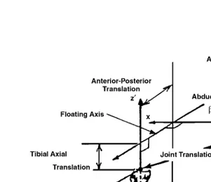
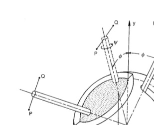
The tibio-femoral joint coordinate system introduced by Grood and Suntay was used to define the rotation and translation vectors that describe the three-dimensional tibio-femoral motions.61 _{This joint}

coordinate system is shown in Fig. 1.1 and consists of an axis (x-axis) that is fixed on the femur (î is a unit vector parallel to the x-axis), an axis (z′-axis) that is fixed on the tibia (kˆ parallel to the z′ ′-axis), and a floating axis perpendicular to these two fixed axes (ê2 is a unit vector parallel to the floating axis).

The three components of the rotation vector include flexion-extension, tibial internal-external, and varus-valgus rotations. Flexion-extension rotations, α, occur around the femoral fixed axis; internal-external tibial rotations, γ, occur about the tibial fixed axis; and varus-valgus rotations, β, (ad-abduction) occur about the floating axis. Using this joint coordinate system, the rotation vector, , describing the orien-tation of the tibial coordinate system with respect to the femoral coordinate system is written as:

= – α î – β ê₂ – γ ˆk

′′′′ (1.1)

This rotation vector can be transformed to the femoral coordinate system, then differentiated with respect to time to yield the angular velocity and angular acceleration vectors of the tibia with respect to the femur. In this analysis, it is assumed that the femur is fixed while the tibia is moving. The locations of the attachment points of the ligamentous structures as well as other bony landmarks are specified on each bone and expressed with respect to a local bony coordinate system. The distances between the tibial and femoral attachment points of the ligamentous structures are calculated in order to determine how the lengths of the ligaments change during motion. Analysis includes expressing the coordinates of each attachment point with respect to one bony coordinate system: the tibia or the femur. This is accomplished by establishing the transformation between the two coordinate systems. The six parameters (three rota-tions and three translarota-tions) describing tibio-femoral morota-tions were used to determine this transformation as follows:

θ

→

R = →Ro + [R]r

→

(1.2)

where →r describes the position vector of a point with respect to the tibial coordinate system, and describes the position vector of the same point with respect to the femoral coordinate system. The vector

Ro

→

is the position vector which locates the origin of the tibial coordinate system with respect to the femoral coordinate system, and [R] is a (3 × 3) rotation matrix given by Grood and Suntay61 _as:

(1.3)

where α is the knee flexion angle, γ is the tibial external rotation angle, and β is (π/2± abduction); positive sign indicates a right knee and negative sign indicates a left knee.

Contact and Geometric Compatibility Conditions

As indicated in the introductory section of this chapter, several methods have been reported in the literature to provide three-dimensional mathematical representations of the articular surfaces of the femur and tibia.12,21,68,124 _{In this model, and for simplicity, geometric primitives are employed. The}

coordinates of a sufficient number of points on the femoral condyles and tibial plateaus of several cadaveric knee specimens were obtained from related studies.67,136 _{A separate mathematical function was}

determined as an approximate representation for each of the medial femoral condyle, the lateral femoral condyle, the medial tibial plateau, and the lateral tibial plateau. The femoral articular surfaces were approximated as parts of spheres, while the tibial plateaus were considered as planar surfaces as shown FIGURE 1.1 Tibio-femoral joint coordinate system. (Source: Rahman, E.M. and Hefzy, M.S., JJBE: Med. Eng. Physics, 20, 4, 276, 1998. With permission from Elsevier Science.)

R

R

[ ]

βcosγ

sin sinβsinγ cosβ

αsinγ

cos

– cosαcosγ sinαsinβ

αcosβcosγ

sin

– –sinαcosβsinγ

αsinγ

sin –sinαcosγ cosαsinβ

αcosβcosγ

cos

– –cosαcosβsinγ

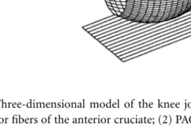
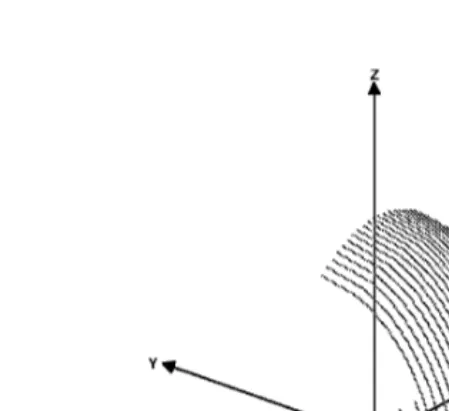
in Figs. 1.2 and 1.3. The equations of the medial and lateral femoral spheres expressed in the femoral coordinate system of axes were written as:

(1.4)

where values of parameters (r, h, k, and l) were obtained as 21, 23.75, 18.0, 12.0 mm and 20.0, 23.0, 16.0, 11.5 mm for the medial and lateral spheres, respectively. The equations of the medial and lateral tibial planes expressed in the tibial coordinate system of axes were written as:

g(x′, y′) = my′ + c (1.5)

where values of parameters (m, c) were obtained as 0.358, 213 mm and –0.341, 212.9 mm for the medial and lateral planes, respectively.

FIGURE 1.2 Three-dimensional model of the knee joint showing the anterior and posterior cruciate ligaments. (1) AAC, Anterior fibers of the anterior cruciate; (2) PAC, posterior fibers of the anterior cruciate; (3) APC, anterior fibers of the posterior cruciate; (4) PPC, posterior fibers of the posterior cruciate.

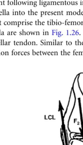
FIGURE 1.3 Three-dimensional model of the knee joint showing the collateral ligaments and the capsular struc-tures. (5) AMC, anterior fibers of the medial collateral; (6) OMC, oblique fibers of the medial collateral; (7) DMC, deep fibers of the medial collateral; (8) LCL, lateral collateral; (9) MCAP, medial fibers of the posterior capsule; (10) LCAP, lateral fibers of the posterior capsule; (11) OPL, oblique popliteal ligament; (12) APL, arcuate popliteal ligament. (Source: Rahman, E.M. and Hefzy, M.S., JJBE: Med. Eng. Physics, 20, 4, 276, 1998. With permission from Elsevier Science.)

This model accomodates two situations: a two-point contact and a single-point contact. Initially, a two-point contact situation is assumed with the femur and tibia in contact on both medial and lateral sides. In the calculations, if one contact force becomes negative, then the two bones within its compart-ment are assumed to be separated, and the single-point contact situation is introduced, thus maintaining contact in the other compartment.

The contact condition requires that the position vectors of each contact point in the femoral and the tibial coordinate systems, →Rc and →rc, respectively, satisfy Eq. (1.2) as follows:

→

Rc = R0 + [R]rc

→

(1.6)

where

(1.6.a)

→

rc = xc′ˆ + yî′ c′ˆj′ ˆ

+ zc′kˆ′ ˆ

(1.6.b)

where xc, yc, zc and xc′, yc′, zc′ are the coordinates of the contact points in the femoral and tibial systems,

respectively. Since contact occurs at points identifiable in both the femoral and tibial articulating surfaces, we can write at each contact point:

zc = f(xc, yc) (7.a)

zc′ = g(xc′, yc′) (7.b)

where f(xc, yc) and g(xc′, yc′) are given by Eqs. (1.4) and (1.5), respectively. Eq. (1.6) can thus be rewritten

as three scalar equations:

xc = x0 + R11xc′ + R12yc′ + R13g(xc′, yc′) (1.8.a)

y_c = y₀ + R₂₁xc′ + R22yc′ + R23g(xc′, yc′) (1.8.b)

f(xc, yc) = z0 + R31xc′ + R32yc′ + R33g(xc′, yc′) (1.8.c)

where Rij is the ijth component of the rotational transformation matrix (R). Eqs. (1.8a) through (1.8c)

constitute a mathematical definition for a contact point. Satisfying these equations at some given point will ensure that it is a contact point. Thus, in the two-point contact version of the model, Eqs. (1.8a) through (1.8c) generate six scalar equations which represent the contact conditions. In the one-point contact version of the model, Eqs. (1.8a) through (1.8c) produce three scalar equations which represent the contact conditions.

The geometric condition of compatibility of rigid bodies requires that a single tangent plane exists to both femoral and tibial surfaces at each contact point. This condition also implies that the normals to the femoral and tibial surfaces at each contact point are always colinear, and their cross product must vanish.

In order to express the geometric compatibility condition in a mathematical form, the position vector of the contact point in the femoral coordinate system (Eq. 1.6.a) is differentiated with respect to the local (x and y) coordinates to obtain two tangent vectors along these local directions. Cross product of these two tangent vectors is then employed to determine the unit vector normal to the femoral surface, , at the contact point. Using Eq. (1.7a), this unit vector is expressed in the femoral coordinate system as:

Rc = xciˆ+ycˆj+zckˆ

(1.9)

A similar analysis is performed to obtain the unit vector normal to the tibial surface, ˆnt′′′′, at the contact point. Using Eq. (1.7b), this unit vector is expressed in the tibial coordinate system as:

(1.10)

Applying the rotational transformation matrix to Eq. (1.10) yields the unit normal vector to the tibial surface, ˆnt, expressed in the femoral coordinate system as:

(1.11)

Since the unit vectors normal to the surfaces of the femur and tibia are colinear, they are equal:

ˆ

nf = ˆnt (1.12)

This vectorial equation is rewritten in a scalar form as:

(1.13a)

(1.13b)

Eqs. (1.13a) and (1.13b) represent the geometric compatibility conditions at each contact point. Thus, for each contact point, two independent scalar equations are written generating four scalar equations to represent the geometric compatibility conditions in the two-point contact situation and two scalar equations to represent the geometric compatibility conditions in the one-point contact situation.

Ligamentous Forces

In this analysis, external loads are applied, and ligamentous and contact forces are then determined. The model includes 12 nonlinear spring elements that represent the different ligamentous structures and the capsular tissue posterior to the knee joint. Four elements represent the respective anterior and posterior fiber bundles of the anterior cruciate ligament (ACL) and the posterior cruciate ligament (PCL); three elements represent the anterior, deep, and oblique fiber bundles of the medial collateral ligament (MCL); one element represents the lateral collateral ligament (LCL); and four elements represent the medial, lateral, and oblique fiber bundles of the posterior part of the capsule (CAP). These twelve elements are shown in Figs. 1.2 and 1.3. The coordinates of the femoral and tibial insertion sites of the different

ligamentous structures were specified according to the data available in the literature.20,36 _These

coordi-nates are listed in Table 1.1.

In the present analysis, ligament wrapping around bone was not taken into consideration. The spring elements representing the ligamentous structures were thus assumed to be line elements extending from the femoral origin to the tibial insertion. These elements were assumed to carry load only when they are in tension, that is, when their length is larger than their slack, unstrained length, Lo. Ligaments exhibit

a region of nonlinear force-elongation relationship, the “toe” region, in the initial stage of ligament strain, then a linear force-elongation relationship in later stages.134 _{A two-piece force-elongation relationship}

was thus used to evaluate the magnitudes of the ligamentous forces.21-23,118,129 _{This relationship is}

com-posed of two regions: a linear region and a parabolic region. The magnitude of the force in the jth

ligamentous element is thus expressed as:

(1.14)

where K1j and K2j are the stiffness coefficients of the jth spring element for the parabolic and linear

regions, respectively, and Lj and Loj are its current and slack lengths, respectively. The strain in the jth

ligamentous element, εj, is given by

(1.15)

and the linear range threshold is specified as ε1 = 0.03.

Values of the stiffness coefficients of the spring elements used to model the different ligamentous structures were estimated according to the data available in the literature21,23,30,93-96,109,118,129,130,133 _{and are}

listed in Table 1.2. The slack length of each spring element is obtained by assuming an extension ratio ej at full extension and using the following relation:

TABLE 1.1 Local Attachment Coordinates of the Ligamentous Structures of the Present Model

Femur Tibia

Ligament x (mm) y (mm) z (mm) x′ (mm) y′ (mm) z′ (mm)

ACL, ant. fibers 7.25 –15.6 21.25 –7.0 5.0 211.25

ACL, post. fibers 7.25 –20.3 19.55 2.0 2.0 212.25

PCL, ant. fibers –4.75 –11.2 14.05 5.0 –30.0 206.25

PCL, post. fibers –4.75 –23.2 15.65 –5.0 –30.0 206.25

MCL, ant. fibers –34.75 –1.0 26.25 –20.0 4.0 171.25

MCL, oblique fibers –34.75 –8.0 24.25 –35.0 –30.0 199.25

MCL, deep fibers –34.75 –5.0 21.25 –35.0 0.0 199.25

LCL 35.25 –15.0 21.25 45.0 –25.0 176.25

Post. capsule, med. –24.75 –38.0 6.25 –25.0 –25.0 181.25

Post. capsule, lat. 25.25 –35.5 8.25 25.0 –25.0 181.25

Post. capsule, oblique popliteal ligament 25.25 –35.5 8.25 –25.0 –25.0 181.25 Post. capsule, arcuate popliteal ligament –24.75 –38.0 6.25 25.0 –25.0 181.25

ACL: Anterior Cruciate Ligament. PCL: Posterior Cruciate Ligament. MCL: Medial Collateral Ligament. LCL: Lateral Collateral Ligament.

(1.16)

to evaluate the spring element’s slack length, Loj, from its length at full extension (which can be calculated

using the coordinates of the attachment points). The values of the extension ratios were specified according to the data available in the literature20,60 _{and are listed in Table 1.3.}

Contact Forces

As the tibia moves with respect to the femur, the contact points also move in the respective medial and TABLE 1.2 Stiffness Coefficients of the Spring Elements Representing the

Ligamentous Structures of the Present Model

Ligament K1 (N/mm2_{) K2 (N/mm}2₎

Post. Capsule, oblique popliteal ligament 21.42 3.00 Post. Capsule, arcuate popliteal ligament 20.82 3.00

ACL: Anterior Cruciate Ligament. PCL: Posterior Cruciate Ligament. MCL: Medial Collateral Ligament. LCL: Lateral Collateral Ligament.

(Source: Rahman, E.M. and Hefzy, M.S., JJBE: Med. Eng. Physics, 20, 4, 276, 1998. With permission from Elsevier Science.)

TABLE 1.3 Extension Ratios at Full Extension of the Ligamentous Structures of the Present Model

Ligament e

Post. capsule, oblique popliteal ligament 1.080 Post. capsule, arcuate popliteal ligament 1.070

ACL: Anterior Cruciate Ligament. PCL: Posterior Cruciate Ligament. MCL: Medial Collateral Ligament. LCL: Lateral Collateral Ligament.

normal to the articular surface. Thus, the contact force applied to the tibia is expressed as: = where Ni is the magnitude of the contact force, and ˆni is the unit vector normal to the tibial surface at the contact point, expressed in the femoral coordinate system. In the two-point contact situation, i = 1, 2 and in the single-point contact situation, i = 1.

Equations of Motion

The equations governing the three-dimensional motion of the tibia with respect to the femur are the second order differential Newton’s and Euler’s equations of motion. Newton’s equations are written in a scalar form, with respect to the femoral fixed system of axes, as:

(1.17)

(1.18)

(1.19)

where m is the mass of the leg, ··xo, ··yo, and ··zo are the components of the linear acceleration of the center

of mass of the leg (in the fixed femoral coordinate system); Wx, Wy, and Wz are the components of the

weight of the leg; and Fex, Fey, and Fez are the components of the external forcing pulse applied to the tibia.

Euler’s equations of motion are written with respect to the moving tibial system of axes which is the tibial centroidal principal system of axes (x′, y′ and z′). Thus, the angular velocity components(θ·x′,θ·y′,

θ·z′)and angular acceleration components (θ··x′, θ··y′, θ··z′), in the Euler equations, are expressed with respect

to this principal system of axes as:

Euler’s equations are written in a scalar form as:

about this centroidal principal axis. The inertial parameters were estimated using the anthropometric data available in the literature.32,34,40,102,120 _{In this analysis, the mass of the leg was taken as m = 4.0 kg.}

Also, the leg was assumed to be a right cylinder; mass moments of inertia were thus calculated as Ix′x′ =

0.0672 kg m2_{, I}

y′y′ = 0.0672 kg m2, and Iz′z′ = 0.005334 kg m2.

In the two point-contact situation, tibio-femoral motions are thus described in terms of six differential equations of motion: Eqs. (1.17) through (1.19) and (1.22) through (1.24), and ten nonlinear algebraic equations [six contact conditions: Eqs. (1.8a through 1.8c), and four geometric compatibility conditions: Eqs. (1.13a) and (1.13b)]. In the one-point contact situation, the ten algebraic equations reduce to five: three contact conditions and two geometric compatibility conditions. The governing system of equations in the two-point contact version of the model thus consists of 16 equations in 16 unknowns: six motion parameters (xo, yo, zo, α, β, and γ); two contact forces (N1 and N2); and eight contact parameters [(xc1,

yc1) and (xc2, yc2): the coordinates of the medial and lateral contact points in the femoral system of axes,

respectively, and (xc1′, yc1′) and (xc2′, yc2′): the coordinates of the medial and lateral contact points in the

tibial system of axes, respectively]. In the one-point contact version of the model, the governing system of equations reduces to 11 equations in 11 unknowns.

1.3 Solution Algorithm

In this formulation, six second order ordinary differential equations (ODEs), Newton’s and Euler’s equations of motion, are written to describe the general motion of the tibia with respect to the femur. Two-point contact is initially assumed. At each contact point five nonlinear algebraic constraints are written to satisfy the contact and compatibility conditions. Thus, this system of equations can be expressed as:

→

F(y→, →y·, y→··, t) = →0 (1.25)

where and . This system has two parts: a differential part and an algebraic part. These

ODE systems are called differential-algebraic equations (DAEs). Numerical methods from the field of ODEs have classically been employed to solve DAE systems.24,53-56,105

The behavior of the numerical methods used to solve a DAE system depends on the DAE’s index. While the existing DAE algorithms are robust enough to handle systems of index one, they encounter difficulties in solving systems of higher indices. The index of a DAE system is the number of times the algebraic constraints need to be differentiated in order to match the order of the differential part of the system and at the same time be able to solve the DAE system for explicit expressions for each of the components of thevector ·→y.55 _{In the present system, N}

1 and N2, two independent variables in vector

→

y, appear only in the differential equations of motion. In order to generate terms that includeN·1 and

N2,

·

with respect to time. These equations are then transformed to third order differential equations. The algebraic constraints are then differentiated thrice with respect to time in order to match the order of the differential part of the system. Consequently, the present system of equations describing the dynamic behavior of the knee joint has an index value of three.

To reduce the order of the system it is rewritten in an equivalent mathematical form which has the same analytical solution but possesses a lower index. The second order time derivatives, accelerations in the equations of motion, are transformed to first order time derivatives of velocity. The system is then augmented with six more first order ordinary differential equations relating the joint motions to the joint velocities. The differential part of the system is transformed to

(1.28c)

(1.29a)

(1.29b)

(1.29c)

The resulting system of equations contains twelve first order ordinary differential equations and ten nonlinear algebraic constraints. It can be written as:

→

F(y→, y→·, t)= →0 (1.30)

where is a vector of dimension (n = 22) containing the 22 independent variables, namely, {xo, yo, zo, α, β, γ, vx, vy, vz, ωα, ωβ, ωγ, xc1, yc1, xc2, yc2, xc1′, yc1′, xc2′, yc2′, N1, and N2}. This is a DAE system of 22

equations to be solved in 22 unknowns. While it is mathematically equivalent to the original system, it has an index of two. To generateN·1 and

·

N2, the equations of motion (which are now of order one) are

to be differentiated once more bringing them to order two. The algebraic constraints are then differen-tiated twice with respect to time so they can match the order of the differential part of the system. Therefore, the new system of equations describing the dynamic behavior of the knee joint has an index value of two.

To solve the DAE system, the algorithm divides the analysis time span into time steps of variable size,

hi, and time stations, ti. From time station tn, the algorithm takes a step forward on time of size hn+1 to

evaluate and and at time station tn+1; that is,

tn+1 = tn + hn +1 (1.31)

At each time station tn+1, components of

→

rn+1

·

are approximated in terms of →yn+1 and at previous time

steps using an integration formula such as a backward differentiation formula (BDF) or a Runge-Kutta (R-K) method. The most popular integration scheme is multistep BDF. This scheme yields:

(1.32)

where k is the order of the formula and (αi, i = 0, k) are the coefficients of the BDF. These coefficients

are determined using generating polynomials such as those defined by Jackson and Sacks-Davis.77 _The

Eq. (1.32) is hence used to eliminate from the system of equations, and the DAE system defined in Eq. (1.30) is transformed to the nonlinear algebraic system:

(1.33)

A

→ variation of the Newton-Raphson iteration technique is then used to solve the nonlinear system for

yn+1.80 _{A solution for the resulting system is thus obtained using the differential form of the}

Newton-Raphson method which includes evaluating iteratively { } by solving the following system of equations:

where is defined by Eq. (1.30). After each iteration is updated according to:

(1.36)

The iterations continue until satisfies a pre-set convergence criterion. A local error test is then carried out to check whether the solution satisfies user-defined error parameters. If the solution is acceptable, the converged values of →yN+1 and are then used with values of and and at the

previous k time stations to evaluate and at tn+2 and the algorithm continues marching on in time.

The stiffness matrix (K) used in step hn+1 is carried on unchanged to step hn+2 unless the algorithm fails

to complete step hn+1 successfully. If the Newton-Raphson iterations fail to converge or the converged

solution fails to satisfy the user-defined error parameters, the algorithm goes back to tn and retakes the

step with an updated stiffness matrix, a smaller step size h, and/or a BDF of a different order.

The initial guess (i = 0) for →yN+1 and (required to begin the Newton-Raphson iterations) is

pre-dicted based on values of at the previous k+1 time stations for a kth order integration formula. A predictor polynomial, which interpolates at the previous k+1 time stations, is used to extrapolate the values of at time station tn+1 while its derivative is used to extrapolate the values of at time station

tn+1. The extrapolation polynomial24 can be written as:

(1.37)

where the recurrence formula of the divided differences is given by

(1.38)

Using Eqs. (1.37) and (1.38), and are estimated by evaluating (t) and (t), respectively, at (t = tn+1). This is called the predictor part of the algorithm while the solution of the nonlinear algebraic

system through Newton-Raphson iterations is called the corrector part of the algorithm. Algorithms which use this approach are called predictor-corrector algorithms.

The initial values of and at t = to (namely, and must be specified in order to completely

define this initial value problem. These initial conditions must be consistent, i.e., they must satisfy the DAE system at time t = t0:

(1.39)

It is important to realize that DAE solvers are very sensitive to the initial conditions. A small inconsistency in the initial conditions, especially for an index two DAE system, can cause the algorithm to diverge in the first step.24

DAE Solvers

Two major computer codes have been developed by the Lawrence Livermore National Laboratory to integrate a DAE using the BDF: the Differential/Algebraic System Solver (DASSL) developed by Petzold106

and the Livermore Solver for Ordinary Differential Equations: Implicit form (LSODI) developed by Hindmarsh and Painter.71 _{Both codes use error-controlled, variable-step, variable-order (integration}

formula) predictor-corrector algorithms to integrate the DAE. Starting at time station (tn), the predictor

extrapolates the values of and at time station (tn+1) based on their values at earlier time stations using

a forward differentiation formula. Then the corrector utilizes a BDF of order ranging from one to five to transform F→(yn+1→ , yn+1→ , tn+1) =

→

0 to the form F→(yn+1→ , tn+1) =

→

0. The two codes differ in the BDF formulas they use and in the step size, order selection, and error control strategies.24 _{Both the load vector}

and the stiffness matrix used in LSODI and DASSL are similar. In both codes, a solution for the resulting system is then obtained using the differential form of the Newton-Raphson method which includes solving Eq. (1.34) iteratively. After each corrector iteration a convergence test is carried; and after convergence, a local error test is also carried.

We have used both LSODI and DASSL to obtain a solution for the present DAE system.5-7 _Some

instabilities were encountered when using the LSODI which is consistent with reports that DASSL is more stable and robust.24 _{Aside from having different error control strategies, the main difference between}

the two codes is that while the LSODI uses a fixed coefficient implementation of the BDF formulas [Eq. (1.32)], the DASSL uses a fixed leading coefficient implementation.24 _{These two techniques allow the}

multistep-fixed step size BDF formulas to accomodate multistep-variable step size applications. In the fixed coefficient implementation, all coefficients of →yn+1–i are unchanged, even when different step sizes, hi, are used. In the fixed leading coefficient implementation, only the first coefficient [that of

→

yn+1 in Eq. (1.32)] does not depend on the step size. We like to point out that Hindmarsh, one of the authors of LSODI, indicated that the LSODI is essentially a stiff differential equation solver, and its use as a DAE solver is only marginal (personal communication). In what follows, we briefly introduce the DASSL software to the reader.

The DASSL computer code is a general purpose DAE solver designed to solve systems of indices zero and one. It can also solve some classes of higher index DAEs including semi-explicit index two systems such as the present DAE system.

Input to the DASSL includes the initial time where the integration begins t = t0, the end of the

integration interval t = tF, , a relative error tolerance vector

→

εrel and an absolute error tolerance

vector εεεε→abs. Each independent variable has a corresponding component in

→

εrel and

→

εabs. User supplied

subroutines evaluate the load vector →F(y→, ·→y, t)and the stiffness matrix [K(y→, t)]. DASSL is called recur-rently in a loop which updates tF until the analysis time span is covered.

The integration formula used by DASSL is a variable step size h variable order k fixed leading coefficient

αs version of the BDF. The order of the BDF can range from one to five.24 At the first time station t0, the

tn, the predictor formula is used to evaluate

→

yn+1,(0), then the corrector iterations are used to correct this value. After each corrector iteration, a convergence test is carried out insuring that the weighted root mean square norm of ∆∆∆∆→y(i) is less than a pre-set convergence constant. The default norm used in DASSL

is a weighted root mean square norm, where the weights depend on the relative and absolute error tolerance vectors and on the value of at the beginning of the step. If the convergence test is not satisfied after four iterations, the step is aborted. The algorithm goes back to station tn, calculates the stiffness

matrix, if it was not current, and repeats the step again. If it fails to converge again, the step size is reduced by a factor of one quarter. If, after ten consecutive step size reductions, the code still fails to take the step, or if at any time h becomes less than the minimum step size, hmin, the code is aborted with a fatal error.

The minimum step size is either specified by the user or calculated by the code in terms of tn, tF, and

the computer roundoff error. If the code is aborted with a fatal error, the user needs to modify the absolute and/or relative error vectors (error tolerance) and restart from the beginning.

If the convergence test is successful, a local error test is carried on the converged solution →yn+1. The test amounts to requiring that the weighted root mean square norm of the difference between the converged solution, yn+1→ , and the predicted solution, →yn+1,(0), be less than the user-defined error toler-ances. If the test fails, the step is aborted and the algorithm goes back to tn and takes the step again.

Regardless of the success of the convergence test (or the local error test), an appropriate order of the BDF and a new step size are calculated before a new step is taken (or before the same step is retaken). The very first time step has to be taken with a BDF of order one (i.e., Euler’s method). Thereafter, and for an initial number of subsequent steps (an initial phase), the code raises the order of the BDF, k, and increases the step size, h. After that initial period, it begins to estimate the errors for different orders by calculating the dominant terms in the remainder of a Taylor series expansion of the solution of order

k – 2, k – 1, k and k + 1, respectively. If the weighted root mean square norm of these quantities (error estimates) decreases with the increase of the order, the order of the BDF, k, is increased by one and if the weighted root mean square norm of the estimates increases with the increase of the order, the order of the BDF, k, is decreased by one. A new step size is then calculated according to the estimate of the local error in the last successful step. The smaller the local error estimate, the larger the next step size will be (in comparison to the previous step). After a successful step, the change in the next step size never exceeds a maximum of double or a minimum of half the previous step size. After an unsuccessful attempted step, which as a result is retaken, the step size is decreased according to the local error estimate in the last successful step. If more than one unsuccessful step has been attempted successively, then the step size is decreased to 25% of its value.

After the local error test fails three times consecutively, the order of the BDF is reduced to one, since a BDF of order one is the most stable fixed leading coefficient BDF at small step size. While trying to satisfy the local error test, if h becomes smaller than hmin the code is aborted with a fatal error; the user

must modify the error tolerance and restart from the beginning.

Load Vector and Stiffness Matrix

(1.58)

(1.59)

(1.60)

(1.61)

Eq. (1.35a) indicates that the stiffness matrix is the partial differential of each component of the load vector with respect to each of the independent variables of the system. This leads to the development of (22 × 22) and (17 × 17) stiffness matrices for the two-point contact and one-point contact situations, respectively. Expressions for the elements forming these matrices are lengthy; they are listed in Reference 7.

1.4 Model Calculations

In a test situation, a sudden impact load was applied at the tibial center of mass with the knee straight. This dynamic load was applied in a posterior direction perpendicular to the tibial mechanical axis. Impact was simulated using sinusoidally decaying forcing pulses with different durations and different magni-tudes. Each pulse is expressed as:

(1.62)

where A and to are amplitude and pulse duration, respectively. Forcing pulses of this form can be simulated

experimentally93 _{and have been used previously as typical representations of the dynamic load in head}

impact analysis.46_{Figs. 1.4 and 1.5 show the sinusoidally decaying forcing pulses of constant duration}

and constant amplitude, respectively, that have been used in the present simulation. Sample results showing the effects of varying pulse magnitude and pulse duration on knee flexion, varus-valgus rotations, internal-external tibial rotations, linear and angular velocities of the tibia, ligamentous forces, and magnitude and location of tibio-femoral contact forces are presented here.

In the analysis, the tibia was assumed to begin its motion from rest (vx = vy = vz = ωα = ωβ = ωγ = 0

at t = t0 = 0 s) while the knee was fully extended (α = 0°, β = 90°, γ = 0° at t = t0 = 0 s). It was found

that the behavior of the system is very sensitive to the location of the initial contact points which required using double precision while performing the computations. On the other hand, even a large error in the initial values of the magnitude of the lateral and medial contact forces did not have an effect on the system’s stability. This is because the behavior of a DAE system is very sensitive to unbalance only in its

algebraic part and not in its differential part. Since neither medial nor lateral contact forces appear in the algebraic part of the DAE, the system is not sensitive to errors in their initial values.

The initial values of the x and y coordinates of the medial contact point in the local femoral and tibial coordinate systems of axes were taken as xc = –16.72913866466 mm and yc = –18.540280082863 mm;

and xc′ = –16.980955 mm and yc′ = –12.8 mm, respectively. The initial values of the x and y coordinates

of the lateral contact point in the local femoral coordinate system were taken as xc = 16.50009371 mm

and yc = –16.00200022911 mm. The medial and lateral contact forces at t = t0 = 0 s were assumed as

150.0 N and 130.0 N, respectively.

Using these assumed values, the coordinates of the tibial origin with respect to the femur at t = t0 =

0 s were calculated using Eq. (1.88), thus satisfying the contact condition at the medial side. The initial values of the x and y coordinates of the lateral contact point in the tibial coordinate system were then calculated using Eq. (1.8) one more time, hence satisfying the contact condition at the lateral side. The unbalance of the system (residual) at t = t0 = 0 s is then determined using Eqs. (1.40) through (1.61).

An iterative procedure is then employed to determine the initial values of the 22 system variables that minimize the initial residual.

FIGURE 1.4 Forcing pulses with different amplitudes and a constant duration of 0.1 s.

Fig. 1.6 shows how the knee flexion angle changes with time for a constant pulse amplitude of 100 N. Increasing pulse duration caused the motion to become faster. This also occurred with increasing pulse amplitude. Figs. 1.7 and 1.8 show how the varus-valgus rotation and the tibial axial rotation angles change with knee flexion, respectively, for pulses with different duration and a constant amplitude of 100 N. The one-point contact model was involved for joint positions with flexion angles larger than the flexion angle at point (A), marked by a star, in each curve in Fig. 1.7 and 1.8. For the rest of the figures presented here, point A is not marked for conciseness.

Fig. 1.7 shows that valgus rotation increased in the first 10° of knee flexion, decreased to zero between 25 and 45° of knee flexion, then varus rotation increased until the knee reached about 60° of flexion, then decreased until 90° of knee flexion. The results indicate that the position at which the knee had zero degrees of varus-valgus rotation changed from 25° of knee flexion to 45° of knee flexion when the pulse duration was increased. Also, Fig. 1.7 shows that increasing the pulse duration caused a decrease in the maximum amount of varus rotation. It was further found (not shown here) that increasing pulse amplitude had the same effects as increasing pulse duration.

FIGURE 1.6 Flexion angle vs. time for different pulses of constant amplitude of 100 N.