Statistical
Methods for
Fuzzy Data
Statistical Methods for
Fuzzy Data
Reinhard Viertl
Vienna University of Technology, Austria
This edition first published 2011 © 2011 John Wiley & Sons, Ltd
Registered office
John Wiley & Sons Ltd, The Atrium, Southern Gate, Chichester, West Sussex, PO19 8SQ, United Kingdom For details of our global editorial offices, for customer services and for information about how to apply for permission to reuse the copyright material in this book please see our website at www.wiley.com. The right of the author to be identified as the author of this work has been asserted in accordance with the Copyright, Designs and Patents Act 1988.
All rights reserved. No part of this publication may be reproduced, stored in a retrieval system, or transmitted, in any form or by any means, electronic, mechanical, photocopying, recording or otherwise, except as permitted by the UK Copyright, Designs and Patents Act 1988, without the prior permission of the publisher. Wiley also publishes its books in a variety of electronic formats. Some content that appears in print may not be available in electronic books.
Designations used by companies to distinguish their products are often claimed as trademarks. All brand names and product names used in this book are trade names, service marks, trademarks or registered trademarks of their respective owners. The publisher is not associated with any product or vendor mentioned in this book. This publication is designed to provide accurate and authoritative information in regard to the subject matter covered. It is sold on the understanding that the publisher is not engaged in rendering professional services. If professional advice or other expert assistance is required, the services of a competent professional should be sought.
Library of Congress Cataloging-in-Publication Data
Viertl, R. (Reinhard)
Statistical methods for fuzzy data / Reinhard Viertl. p. cm.
Includes bibliographical references and index. ISBN 978-0-470-69945-4 (cloth)
1. Fuzzy measure theory. 2. Fuzzy sets. 3. Mathematical statistics. I. Title. QA312.5.V54 2010
515′.42–dc22
2010031105 A catalogue record for this book is available from the British Library.
Print ISBN: 978-0-470-69945-4 ePDF ISBN: 978-0-470-97442-1 oBook ISBN: 978-0-470-97441-4 ePub ISBN: 978-0-470-97456-8
Contents
Preface xi
Part I FUZZY INFORMATION
1
1 Fuzzy data 3
1.1 One-dimensional fuzzy data 3
1.2 Vector-valued fuzzy data 4
1.3 Fuzziness and variability 4
1.4 Fuzziness and errors 4
1.5 Problems 5
2 Fuzzy numbers and fuzzy vectors 7
2.1 Fuzzy numbers and characterizing functions 7
2.2 Vectors of fuzzy numbers and fuzzy vectors 14
2.3 Triangular norms 16
2.4 Problems 18
3 Mathematical operations for fuzzy quantities 21
3.1 Functions of fuzzy variables 21
3.2 Addition of fuzzy numbers 23
3.3 Multiplication of fuzzy numbers 25
3.4 Mean value of fuzzy numbers 25
3.5 Differences and quotients 27
3.6 Fuzzy valued functions 27
3.7 Problems 28
Part II DESCRIPTIVE STATISTICS FOR FUZZY DATA
31
4 Fuzzy samples 33
4.1 Minimum of fuzzy data 33
4.2 Maximum of fuzzy data 33
4.3 Cumulative sum for fuzzy data 34
vi CONTENTS
5 Histograms for fuzzy data 37
5.1 Fuzzy frequency of a fixed class 37
5.2 Fuzzy frequency distributions 38
5.3 Axonometric diagram of the fuzzy histogram 40
5.4 Problems 41
6 Empirical distribution functions 43
6.1 Fuzzy valued empirical distribution function 43
6.2 Fuzzy empirical fractiles 45
6.3 Smoothed empirical distribution function 45
6.4 Problems 47
7 Empirical correlation for fuzzy data 49
7.1 Fuzzy empirical correlation coefficient 49
7.2 Problems 52
Part III FOUNDATIONS OF STATISTICAL
INFERENCE WITH FUZZY DATA
53
8 Fuzzy probability distributions 55
8.1 Fuzzy probability densities 55
8.2 Probabilities based on fuzzy probability densities 56
8.3 General fuzzy probability distributions 57
8.4 Problems 58
9 A law of large numbers 59
9.1 Fuzzy random variables 59
9.2 Fuzzy probability distributions induced by fuzzy random variables 61
9.3 Sequences of fuzzy random variables 62
9.4 Law of large numbers for fuzzy random variables 63
9.5 Problems 64
10 Combined fuzzy samples 65
10.1 Observation space and sample space 65
10.2 Combination of fuzzy samples 66
10.3 Statistics of fuzzy data 66
10.4 Problems 67
Part IV CLASSICAL STATISTICAL INFERENCE
FOR FUZZY DATA
69
11 Generalized point estimators 71
CONTENTS vii
11.2 Sample moments 73
11.3 Problems 74
12 Generalized confidence regions 75
12.1 Confidence functions 75
12.2 Fuzzy confidence regions 76
12.3 Problems 79
13 Statistical tests for fuzzy data 81
13.1 Test statistics and fuzzy data 81
13.2 Fuzzy p-values 82
13.3 Problems 86
Part V BAYESIAN INFERENCE AND FUZZY
INFORMATION
87
14 Bayes’ theorem and fuzzy information 91
14.1 Fuzzy a priori distributions 91
14.2 Updating fuzzy a priori distributions 92
14.3 Problems 96
15 Generalized Bayes’ theorem 97
15.1 Likelihood function for fuzzy data 97
15.2 Bayes’ theorem for fuzzy a priori distribution and fuzzy data 97
15.3 Problems 101
16 Bayesian confidence regions 103
16.1 Bayesian confidence regions based on fuzzy data 103
16.2 Fuzzy HPD-regions 104
16.3 Problems 106
17 Fuzzy predictive distributions 107
17.1 Discrete case 107
17.2 Discrete models with continuous parameter space 108
17.3 Continuous case 110
17.4 Problems 111
18 Bayesian decisions and fuzzy information 113
18.1 Bayesian decisions 113
18.2 Fuzzy utility 114
18.3 Discrete state space 115
18.4 Continuous state space 116
viii CONTENTS
Part VI REGRESSION ANALYSIS AND FUZZY
INFORMATION
119
19 Classical regression analysis 121
19.1 Regression models 121
19.2 Linear regression models with Gaussian dependent variables 125
19.3 General linear models 128
19.4 Nonidentical variances 131
19.5 Problems 132
20 Regression models and fuzzy data 133
20.1 Generalized estimators for linear regression models based on the
extension principle 134
20.2 Generalized confidence regions for parameters 138
20.3 Prediction in fuzzy regression models 138
20.4 Problems 139
21 Bayesian regression analysis 141
21.1 Calculation of a posteriori distributions 141
21.2 Bayesian confidence regions 142
21.3 Probabilities of hypotheses 142
21.4 Predictive distributions 142
21.5 A posteriori Bayes estimators for regression parameters 143
21.6 Bayesian regression with Gaussian distributions 144
21.7 Problems 144
22 Bayesian regression analysis and fuzzy information 147
22.1 Fuzzy estimators of regression parameters 148
22.2 Generalized Bayesian confidence regions 150
22.3 Fuzzy predictive distributions 150
22.4 Problems 151
Part VII FUZZY TIME SERIES
153
23 Mathematical concepts 155
23.1 Support functions of fuzzy quantities 155
23.2 Distances of fuzzy quantities 156
23.3 Generalized Hukuhara difference 161
24 Descriptive methods for fuzzy time series 167
24.1 Moving averages 167
24.2 Filtering 169
24.2.1 Linear filtering 169
CONTENTS ix
24.3 Exponential smoothing 175
24.4 Components model 176
24.4.1 Model without seasonal component 177
24.4.2 Model with seasonal component 177
24.5 Difference filters 182
24.6 Generalized Holt–Winter method 184
24.7 Presentation in the frequency domain 186
25 More on fuzzy random variables and fuzzy random vectors 189
25.1 Basics 189
25.2 Expectation and variance of fuzzy random variables 190
25.3 Covariance and correlation 193
25.4 Further results 196
26 Stochastic methods in fuzzy time series analysis 199
26.1 Linear approximation and prediction 199
26.2 Remarks concerning Kalman filtering 212
Part VIII APPENDICES
215
A1 List of symbols and abbreviations 217
A2 Solutions to the problems 223
A3 Glossary 245
A4 Related literature 247
References 251
Preface
Statistics is concerned with the analysis of data and estimation of probability distribu-tion and stochastic models. Therefore the quantitative descripdistribu-tion of data is essential for statistics.
In standard statistics data are assumed to be numbers, vectors or classical func-tions. But in applications real data are frequently not precise numbers or vectors, but often more or lessimprecise, also calledfuzzy. It is important to note that this kind of uncertainty is different from errors; it is the imprecision of individual observations or measurements.
Whereas counting data can be precise, possibly biased by errors, measurement data of continuous quantities like length, time, volume, concentrations of poisons, amounts of chemicals released to the environment and others, are always not precise real numbers but connected with imprecision.
In measurement analysis usually statistical models are used to describe data uncertainty. But statistical models are describing variability and not the imprecision of individual measurement results. Therefore other models are necessary to quantify the imprecision of measurement results.
For a special kind of data, e.g. data from digital instruments, interval arithmetic can be used to describe the propagation of data imprecision in statistical inference. But there are data of a more general form than intervals, e.g. data obtained from analog instruments or data from oscillographs, or graphical data like color intensity pictures. Therefore it is necessary to have a more general numerical model to describe measurement data.
The most up-to-date concept for this is special fuzzy subsets of the setRof real numbers, or special fuzzy subsets of thek-dimensional Euclidean spaceRkin the case
of vector quantities. These special fuzzy subsets ofRare called nonprecise numbers in the one-dimensional case and nonprecise vectors in thek-dimensional case fork>1. Nonprecise numbers are defined by so-calledcharacterizing functionsand nonprecise vectors by so-called vector-characterizing functions. These are generalizations of indicator functions of classical sets in standard set theory. The concept of fuzzy numbers from fuzzy set theory is too restrictive to describe real data. Therefore nonprecise numbersare introduced.
xii PREFACE
There are also other approaches for the analysis of fuzzy data. Here an approach from the viewpoint of applications is used. Other approaches are mentioned in Ap-pendix A4.
Besides fuzziness of data there is also fuzziness of a priori distributions in Bayesian statistics. So called fuzzy probability distributionscan be used to model nonprecise a priori knowledge concerning parameters in statistical models.
In the text the necessary foundations of fuzzy models are explained and basic sta-tistical analysis methods for fuzzy samples are described. These include generalized classical statistical procedures as well as generalized Bayesian inference procedures. A software system for statistical analysis of fuzzy data (AFD) is under develop-ment. Some procedures are already available, and others are in progress. The available software can be obtained from the author.
Last but not least I want to thank all persons who contributed to this work: Dr D. Hareter, Mr H. Schwarz, Mrs D. Vater, Dr I. Meliconi, H. Kay, P. Sinha-Sahay and B. Kaur from Wiley for the excellent cooperation, and my wife Dorothea for preparing the files for the last two parts of this book.
I hope the readers will enjoy the text.
Part I
FUZZY INFORMATION
Fuzzy information is a special kind of information and information is an omnipresent word in our society. But in general there is no precise definition of information.
However, in the context of statistics which is connected to uncertainty, a possi-ble definition of information is the following: Information is everything which has influence on the assessment of uncertainty by an analyst. This uncertainty can be of different types: data uncertainty, nondeterministic quantities, model uncertainty, and uncertainty of a priori information.
Measurement results and observational data are special forms of information. Such data are frequently not precise numbers but more or less nonprecise, also called fuzzy. Such data will be considered in the first chapter.
Another kind of information is probabilities. Standard probability theory is con-sidering probabilities to be numbers. Often this is not realistic, and in a more general approach probabilities are considered to be so-calledfuzzy numbers.
1
Fuzzy data
All kinds of data which cannot be presented as precise numbers or cannot be precisely classified are called nonprecise orfuzzy. Examples are data in the form of linguistic descriptions like high temperature, low flexibility and high blood pressure. Also, precision measurement results of continuous variables are not precise numbers but alwaysmore or less fuzzy.
1.1
One-dimensional fuzzy data
Measurement results of one-dimensional continuous quantities are frequently ideal-ized to be numbers times a measurement unit. However, real measurement results of continuous quantities are never precise numbers but always connected with un-certainty. Usually this uncertainty is considered to be statistical in nature, but this is not suitable since statistical models are suitable to describe variability. For a sin-gle measurement result there is no variability, therefore another method to model the measurement uncertainty of individual measurement results is necessary. The best up-to-date mathematical model for that are so-calledfuzzy numberswhich are described in Section 2.1 [cf. Viertl (2002)].
Examples of one-dimensional fuzzy data are lifetimes of biological units, length measurements, volume measurements, height of a tree, water levels in lakes and rivers, speed measurements, mass measurements, concentrations of dangerous substances in environmental media, and so on.
A special kind of one-dimensional fuzzy data are data in the form of intervals [a;b]⊆R. Such data are generated by digital measurement equipment, because they have only a finite number of digits.
4 STATISTICAL METHODS FOR FUZZY DATA
Figure 1.1 Variability and fuzziness.
1.2
Vector-valued fuzzy data
Many statistical data are multivariate, i.e. ideally the corresponding measurement results are real vectors (x1, . . . ,xk)∈Rk. In applications such data are frequently
not precise vectors but to some degree fuzzy. A mathematical model for this kind of data is so-calledfuzzy vectorswhich are formalized in Section 2.2.
Examples of vector valued fuzzy data are locations of objects in space like positions of ships on radar screens, space–time data, multivariate nonprecise data in the form of vectors (x∗
1, . . . ,x∗n) of fuzzy numbersx
∗
i.
1.3
Fuzziness and variability
In statistics frequently so-called stochastic quantities (also called random variables) are observed, where the observed results are fuzzy. In this situation two kinds of uncertainty are present: Variability, which can be modeled by probability distribu-tions, also called stochastic models, and fuzziness, which can be modeled by fuzzy numbers and fuzzy vectors, respectively. It is important to note that these are two different kinds of uncertainty. Moreover it is necessary to describe fuzziness of data in order to obtain realistic results from statistical analysis. In Figure 1.1 the situation is graphically outlined.
Real data are also subject to a third kind of uncertainty: errors. These are the subject of Section 1.4.
1.4
Fuzziness and errors
FUZZY DATA 5
error, i.e.
y=x+e.
The error is considered as the realization of another stochastic quantity. These kinds of errors are denoted as random errors.
For one-dimensional quantities, all three quantities x, y, and e are, after the experiment, real numbers. But this is not suitable for continuous variables because the observed valuesyare fuzzy.
It is important to note that all three kinds of uncertainty are present in real data. Therefore it is necessary to generalize the mathematical operations for real numbers to the situation of fuzzy numbers.
1.5
Problems
(a) Find examples of fuzzy numerical data which are not given in Section 1.1 and Section 1.2.
(b) Work out the difference between stochastic uncertainty and fuzziness of individ-ual observations.
(c) Make clear how data in the form of intervals are obtained by digital measurement devices.
2
Fuzzy numbers and fuzzy
vectors
Taking care of the fuzziness of data described in Chapter 1 it is necessary to have a mathematical model to describe such data in a quantitative way. This is the subject of Chapter 2.
2.1
Fuzzy numbers and characterizing functions
In order to model one-dimensional fuzzy data the best up-to-date mathematical model is so-called fuzzy numbers.
Definition 2.1: A fuzzy number x∗ is determined by its so-called characterizing
functionξ(·) which is a real function of one real variablexobeying the following:
(1) ξ :R→[0; 1].
(2) ∀δ∈(0; 1] the so-calledδ-cutCδ(x∗) := {x∈R:ξ(x)≥δ}is a finite union
of compact intervals, [aδ,j;bδ,j], i.e.Cδ(x∗)= kδ
j=1
[aδ,j;bδ,j]= ∅.
(3) The support ofξ(·), defined by supp[ξ(·)] := {x∈R:ξ(x)>0}is bounded.
The set of all fuzzy numbers is denoted byF(R).
For the following and for applications it is important that characterizing functions can be reconstructed from the family (Cδ(x∗); δ∈(0; 1]), in the way described in
Lemma 2.1.
8 STATISTICAL METHODS FOR FUZZY DATA
Lemma 2.1:For the characterizing functionξ(·) of a fuzzy numberx∗the following holds true:
ξ(x)=max
δ·ICδ(x∗)(x) :δ∈[0; 1] ∀x∈R
Proof:For fixedx0∈Rwe have
δ·ICδ(x∗)(x0)=δ·I{x:ξ(x)≥δ}(x0)=
δ for ξ(x0)≥δ 0 for ξ(x0)< δ.
Therefore we have for everyδ∈[0;1]
δ·ICδ(x∗)(x0)≤ξ(x0),
and further
sup
δ·ICδ(x∗)(x0) :δ∈[0; 1]≤ξ(x0).
On the other hand we have forδ0=ξ(x0):
δ0·ICδ0(x∗)(x0)=δ0and therefore
sup
δ·ICδ(x∗)(x0) :δ∈[0; 1]
≥δ0which implies sup
δ·ICδ(x∗)(x0) :δ∈[0; 1]
=max
δ·ICδ(x∗)(x0) :δ∈[0; 1]
=δ0.
Remark 2.1:In applications fuzzy numbers are represented by a finite number of δ-cuts.
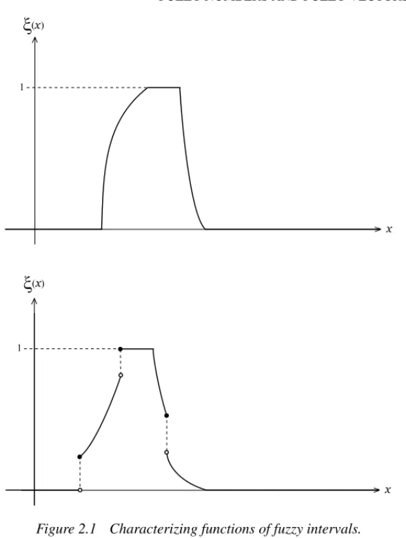
Special types of fuzzy numbers are useful to define so-called fuzzy probability distribution. These kinds of fuzzy numbers are denoted as fuzzy intervals.
Definition 2.2:A fuzzy number is called afuzzy intervalif all itsδ-cuts are non-empty closed bounded intervals.
In Figure 2.1 examples of fuzzy intervals are depicted.
The set of all fuzzy intervals is denoted byFI(R).
Remark 2.2:Precise numbersx0∈Rare represented by its characterizing function I{x0}(·), i.e. the one-point indicator function of the set{x0}. For this characterizing
function the δ-cuts are the degenerated closed interval [x0;x0].= {x0}. Therefore precise data are specialized fuzzy numbers.
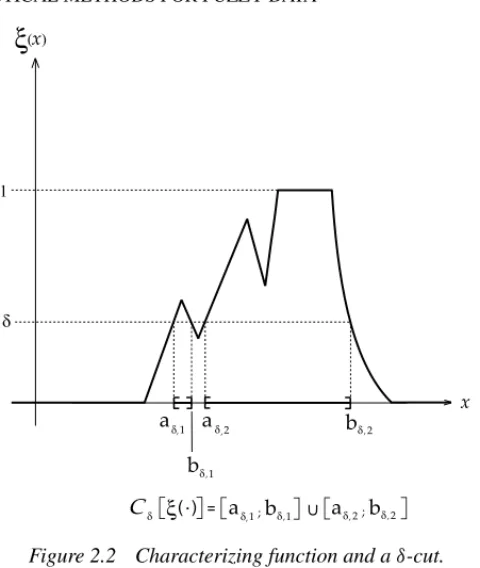
In Figure 2.2 theδ-cut for a characterizing function is explained.
Special types of fuzzy intervals are so-calledLR- fuzzy numbers which are defined by two functionsL : [0;∞)→[0; 1] andR: [0,∞)→[0,1] obeying the following:
(1) L(·) andR(·) are left-continuous.
(2) L(·) andR(·) have finite support.
FUZZY NUMBERS AND FUZZY VECTORS 9
Figure 2.1 Characterizing functions of fuzzy intervals.
Using these functions the characterizing functionξ(·) of anLR-fuzzy interval is defined by:
ξ(x)= ⎧ ⎪ ⎪ ⎪ ⎪ ⎨
⎪ ⎪ ⎪ ⎪ ⎩
L m−s−x l
for x<m−s
1 for m−s≤x≤m+s
R m−s−x r
for x>m+s,
wherem,s,l,r are real numbers obeyings≥0,l >0,r >0. Such fuzzy numbers are denoted bym,s,l,rLR.
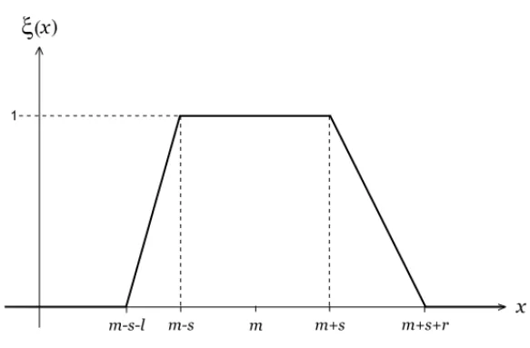
A special type ofLR-fuzzy numbers are the so-calledtrapezoidal fuzzy numbers, denoted byt∗(m,s,l,r) with
10 STATISTICAL METHODS FOR FUZZY DATA
Figure 2.2 Characterizing function and aδ-cut.
The corresponding characterizing function oft∗(m,s,l,r) is given by
ξ(x)= ⎧ ⎪ ⎪ ⎪ ⎪ ⎨
⎪ ⎪ ⎪ ⎪ ⎩
x−m+s+l
l for m−s−l≤x<m−s
1 for m−s≤x ≤m+s
m+s+r−x
r for m+s<x≤m+s+r
0 otherwise.
In Figure 2.3 the shape of a trapezoidal fuzzy number is depicted.
Theδ-cuts of trapezoidal fuzzy numbers can be calculated easily using the so-called pseudo-inverse functionsL−1(·) andR−1(·) which are given by
L−1(δ)=max{x ∈R:L(x)≥δ} R−1(δ)=max{x ∈R: R(x)≥δ}
Lemma 2.2:Theδ-cutsCδ(x∗) of anLR-fuzzy numberx∗are given by
FUZZY NUMBERS AND FUZZY VECTORS 11
Figure 2.3 Trapezoidal fuzzy number.
Proof: The left boundary of Cδ(x∗) is determined by min{x:ξ(x)≥δ}. By the definition ofLR-fuzzy numbers forl>0 we obtain
min{x:ξ(x)≥δ} =min
x:L m−s−x l
≥δandx<m−s
=min
x: m−s−x
l ≤L
−1(δ) and x<m−s
=min
x:x≥m−s−l L−1(δ) and x<m−s
=m−s−l L−1(δ).
The proof for the right boundary is analogous.
An important topic is how to obtain the characterizing function of fuzzy data. There is no general rule for that, but for different important measurement situations procedures are available.
For analog measurement equipment often the result is obtained as a light point on a screen. In this situation the light intensity on the screen is used to obtain the characterizing function. For one-dimensional quantities the light intensity h(·) is normalized, i.e.
ξ(x) := h(x)
max{h(x) :x∈R} ∀x∈R,
andξ(·) is the characterizing function of the fuzzy observation.
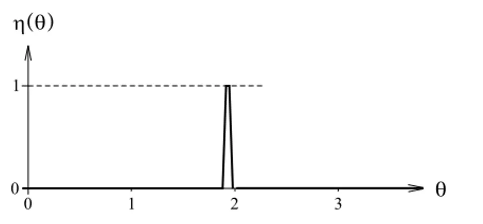
For light points on a computer screen the functionh(·) is given on finitely many pixels x1, . . . ,xN with intensitiesh(xi),i =1(1)N. In order to obtain the
12 STATISTICAL METHODS FOR FUZZY DATA
the characterizing functionξ(·) is obtained in the following way:
Based on the functionη(·) the valuesξ(x) are defined for allx∈Rby
Remark 2.3:ξ(·) is a characterizing function of a fuzzy number.
For digital measurement displays the results are decimal numbers with a finite number of digits. Let the resulting number bey, then the remaining (infinite many) decimals are unknown. The numerical information contained in the result is an interval [x;x], wherexis the real number obtained fromyby taking the remaining decimals all to be 0, andxis the real number obtained fromyby taking the remaining decimals all to be 9. The corresponding characterizing function of this fuzzy number is the indicator functionI[x;x](·) of the closed interval [x;x].
Therefore the characterizing functionξ(·) is given by its values
FUZZY NUMBERS AND FUZZY VECTORS 13
If the measurement result is given by a color intensity picture, for example diameters of particles, the color intensity is used to obtain the characterizing function ξ(·). Leth(·) be the color intensity describing the boundary then the derivativeh′(·) ofh(·) is used, i.e.
ξ(x) :=
h′(x)
max{|h′(x)|:x ∈R} ∀x∈R.
An example is given in Figure 2.4.
For color intensity pictures on digital screens a discrete version for step functions can be applied.
Let {x1, . . . ,xN}be the discrete values of the variable and h(xi) be the color
intensities at positionxi as before, andxthe constant distance between the points
xi. Then the discrete analog of the derivativeh′(·) is given by the step functionη(·)
14 STATISTICAL METHODS FOR FUZZY DATA
which is constant in the intervals
xi−2x;xi+2x:
η(x) := |h(xi−ε)−h(xi+ε)| with 0 < ε <
x 2
The corresponding characterizing functionξ(·) of the fuzzy boundary is given by
ξ(x) := η(x)
max{η(x) :x∈R} for allx∈R.
The functionξ(·) is a characterizing function of a fuzzy number.
2.2
Vectors of fuzzy numbers and fuzzy vectors
For multivariate continuous data measurement results are fuzzy too. In the idealized case the result is ak-dimensional real vector (x1, . . . ,xk). Depending on the problem
two kinds of situations are possible.
The first is when the individual values of the variablesxi are fuzzy numbersxi∗.
Then a vector (x∗
1, . . . ,xk∗) of fuzzy numbers is obtained. This vector is determined
bykcharacterizing functionsξ1(·), . . . , ξk(·). Methods to obtain these characterizing
functions are described in Section 2.1.
The second situation yields a fuzzy version of a vector, for example the position of a ship on a radar screen. In the idealized case the position is a two-dimensional vector (x,y)∈R2. In real situation the position is characterized by a light point on the screen which is not a precise vector. The result is a so-calledfuzzy vector, denoted as (x,y)∗.
The mathematical model of a fuzzy vector is given in the following definition, using the notationx =(x1, . . . ,xk).
Definition 2.3:Ak-dimensional fuzzy vectorx∗is determined by its so-called
vector-characterizing functionξ(, . . . ,) which is a real function ofkreal variablesx1, . . . ,xk
obeying the following:
(1) ξ :Rk→[0; 1].
(2) The support ofξ(, . . . ,) is a bounded set.
(3) ∀δ∈(0; 1] the so-calledδ-cutCδ
x∗
:=
x∈Rk:ξ x
≥δ
is non-empty, bounded, and a finite union of simply connected and closed bounded sets.
The set of allk-dimensional fuzzy vectors is denoted byF(Rk).
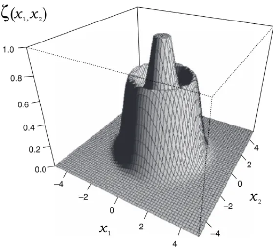
In Figure 2.5 a vector-characterizing function of a two-dimensional fuzzy vector is depicted.
FUZZY NUMBERS AND FUZZY VECTORS 15
1.0
0.8
0.6
0.4
0.2
0.0 –4
–4 –2
–2 0
0
2
2
4
4
Figure 2.5 Vector-characterizing function.
For statistical inference specialized fuzzy vectors are important, the so-called fuzzyk-dimensional intervals.
Definition 2.4:Ak-dimensional fuzzy vector is called ak-dimensional fuzzy interval if allδ-cuts are simply connected compact sets.
An example of a two-dimensional fuzzy interval is given in Figure 2.6.
Lemma 2.3:The vector-characterizing functionξ(, . . . ,) of a fuzzy vectorx∗can be
reproduced by itsδ-cuts in the following way:
ξ x
=maxδ·ICδ(x∗)
x
: δ ∈(0; 1] ∀x∈ Rk The proof is similar to the proof of Lemma 2.1.
Again it is important how to obtain the vector-characterizing function of a fuzzy vector. There is no general rule for this but some methodology.
For two-dimension fuzzy vectorsx∗ =(x,y)∗given by light intensities the
vector-characterizing function ξ(·) of x∗ is obtained from the values h(x,y) of the light intensity by
ξ (x,y) := h(x,y)
max
16 STATISTICAL METHODS FOR FUZZY DATA
Figure 2.6 Fuzzy two-dimensional interval.
If only fuzzy values of the componentsxiof ak-dimensional vector (xi, . . . ,xk)
are available, i.e. x∗
i with corresponding characterizing function ξi(·),i =1(1)n,
these characterizing functions can be combined into a vector-characterizing function of ak-dimensional fuzzy vector using so-calledtriangular norms. Details of this are explained in Section 2.3.
2.3
Triangular norms
A vector (x∗
1, . . . ,xk∗) of fuzzy numbersx
∗
i is not a fuzzy vector. For the generalization
of statistical inference, functions defined on sample spaces are essential. Therefore it is basic to form fuzzy elements in the sample spaceM×. . .×M, whereM denotes the observation space of a random quantity. These fuzzy elements are fuzzy vectors. By this it is necessary to form fuzzy vectors from fuzzy samples. This is done by applying so-called triangular norms, also called t-norms.
Definition 2.5:A functionT : [0; 1]×[0; 1]→[0; 1] is called a t-norm, if for all x,y,z,∈[0; 1] the following conditions are fulfilled:
(1) T(x,y)=T(y,x) commutativity.
(2) T(T(x,y),z)=T(x,T(y,z)) associativity.
(3) T(x,1)=x.
FUZZY NUMBERS AND FUZZY VECTORS 17
Examples of t-norms are:
(a) Minimum t-norm
T(x,y)=min{x,y} ∀x,y∈[0; 1]
(b) Product t-norm
T(x,y)=x·y ∀x,y∈[0; 1]
(c) Limited sum t-norm
T(x,y)=max{x+y−1,0} ∀x,y∈[0; 1]
Remark 2.5:For statistical and algebraic calculations with fuzzy data the minimum t-norm is optimal. For the combination of fuzzy components of vector data in some examples the product t-norm is more suitable.
For more details on mathematical aspects of t-norms see Klementet al.(2000). Based on t-norms the combination of fuzzy numbers into a fuzzy vector is pos-sible. For two fuzzy numbersx∗andy∗with corresponding characterizing functions
ξ(·) andη(·) a fuzzy vectorx∗=(x,y)∗is given by its vector-characterizing function
ξ(·). The valuesξ(x,y) are defined based on a t-normT by
ξ(x,y) :=T(ξ(x), η(y)) ∀(x,y)∈R2·
By the associativity of t-norms this can be extended also to k fuzzy numbers x∗
1, . . . ,xk∗with corresponding characterizing functionsξ1(·), . . . , ξk(·) in the
follow-ing way:
ξ(x1, . . . ,xk) :=T(ξ1(x1),T(· · ·,T (ξk−1(xk−1), ξk(xk))· · ·))∀(x1, . . . ,xk)∈Rk
Remark 2.6:For the minimum t-norm it follows
ξ(x1, . . . ,xk)=min{ξ1(x1), . . . , ξk(xk)} ∀(x1, . . . ,xk)∈Rk.
For the minimum t-norm theδ-cuts of the combined fuzzy vector are very easy to obtain. This is shown in Proposition 2.1.
Proposition 2.1: For k fuzzy numbers x∗1, . . . ,xk∗ with characterizing functions ξ1(·), . . . , ξk(·) the δ-cuts Cδ(x∗) of the fuzzy vector x∗, combined by the
mini-mum t-norm are the Cartesian products of theδ-cutsCδ(xi∗) of the fuzzy numbers
x∗
1, . . . ,xk∗:
18 STATISTICAL METHODS FOR FUZZY DATA
Figure 2.7 Combination of two fuzzy numbers.
Proof:Letξ(., . . . ,.) be the vector-characterizing function ofx∗. Then forδ∈(0; 1]
theδ-cut Cδ(x∗) obeys
Cδ x∗
=
x ∈Rk:ξ x
≥δ
=
(x1,· · ·,xk)∈Rk: min{ξ1(x1),· · ·, ξk(xk)} ≥δ
=(x1,· · ·,xk)∈Rk:ξi(xi)≥δ ∀i =1 (1)k
= Xk
i=1
{xi ∈R:ξi(xi)≥δ} = k
X
i=1Cδ
xi∗.
In Figure 2.7 this is explained graphically.
Remark 2.7:The minimum t-norm is also the natural t-norm for the generalization of algebraic operations to the system of fuzzy numbers.
2.4
Problems
FUZZY NUMBERS AND FUZZY VECTORS 19
(b) Let the color intensity for a one-dimensional quantity be given by the following function:
Color
Find the characterizing function of the fuzzy boundary between low color intensity and maximal color intensity using the method described in Section 2.1. (c) Calculate theδ-cuts of a fuzzy vector with vector-characterizing function
ξ(x,y)=I[a1;b1]×[a2;b2](x,y) ∀(x,y)∈R
2.
(d) Explain that the combination of fuzzy numbers, based on the minimum t-norm, yields a fuzzy vector.
3
Mathematical operations for
fuzzy quantities
The extension of algebraic operations to fuzzy numbers is based on the so-called extension principle from fuzzy set theory. This extension principle is a method to extend classical functions f : M →Nto the situation, when the argument is a fuzzy element inM.
3.1
Functions of fuzzy variables
In order to extend statistical functions f(x1, . . .xn) of samplesx1, . . . ,xnthe
follow-ing definition is useful.
Definition 3.1:(Extension principle): Let f :M → Nbe an arbitrary function from M to N. For a fuzzy element x∗ in M, characterized by an arbitrary membership function µ:M →[0; 1] the generalized (fuzzy) value y∗= f(x∗) for the fuzzy argument valuex∗is the fuzzy elementy∗inN whose membership functionψ(·) is defined by
ψ(y) :=
sup{µ(x) :x∈M, f(x)=y} if∃x: f(x)=y
0 if∃/x: f(x)=y
∀y∈N.
Remark 3.1:The extension principle is a natural way to model the propagation of imprecision. It corresponds to the engineering principle ‘to be on the safe side’.
The following statements are important for the generalization of statistical functions.
22 STATISTICAL METHODS FOR FUZZY DATA
Proposition 3.1:Let f : M →N be a classical function, andx∗a fuzzy element of M with membership functionµ(·). Then the fuzzy element y∗= f(x∗) defined by the extension principle obeys the following:
f Cδ(x∗)
⊆Cδ(y∗) ∀δ∈(0; 1]
Proof:Cδ(y∗)= {y∈ N :ψ(y)≥δ}whereψ(·) is defined as in Definition 3.1. By f(Cδ(x∗))= {f(x) :x∈Cδ(x∗)}, for y∈(Cδ(x∗)) there exists x∈(Cδ(x∗)) with f(x)=y. Thereforeµ(x)≥δand sup{µ(x) : f(x)=y} ≥δand y∈(Cδ(y∗)).
Classical statistical functions are frequently functions f :Rn →R. If such
statis-tics are continuous functions, the following theorem holds.
Theorem 3.1: Let f :Rn →R be a continuous function and x∗ a fuzzy n-dimensional interval. Then the following is true:
(a) f(x∗) defined by the extension principle is a fuzzy interval.
(b) Cδ (0; 1]. By Proposition 3.1 we have
f
≥δ. Therefore there exists a sequence xn∈ f−1({y}),n ∈Nwith sup ξ(xn) :n∈N has accumulation pointδ. Therefore there exists a convergent subsequencezn,n∈N,
and by the compactness of f−1({y})∩Cδ(x∗) the limitz
0of this subsequence be-longs to f−1({y})∩Cδ(x∗).By lim
n→∞ξ(zn)=δ we obtainξ(z0)=δ and therefore ψ(y)=δ, andy∈ f(Cδ(x∗)). By definition of fuzzy vectorsCδ(x∗) is compact and connected. By the continuity of f(·) follows that f(Cδ(x∗)) is connected and compact. Therefore it is a closed finite interval.
Corollary 3.1:For continuous function f :R→Rand fuzzy intervalx∗, the fuzzy value f(x∗) is a fuzzy interval with
MATHEMATICAL OPERATIONS FOR FUZZY QUANTITIES 23
Figure 3.1 Continuous function of a fuzzy interval.
Remark 3.2:The resulting characterizing function in Figure 3.1 is not continuous, although bothξ(·) and f(·) are continuous.
3.2
Addition of fuzzy numbers
Let x1∗ andx2∗ be two fuzzy numbers with corresponding characterizing functions ξ1(·) andξ2(·). The generalized addition operation⊕for fuzzy numbers has to obey two demands: First it has to generalize the addition of real numbers, and secondly it has to generalize interval arithmetic.
For fuzzy intervalsx∗
1andx2∗the generalized addition can be defined usingδ-cuts. LetCδ(x1∗)=[aδ,1;bδ,1] andCδ(x2∗)=[aδ,2;bδ,2] ∀δ∈[0; 1] then theδ-cut of the fuzzy sumx∗
1 ⊕x2∗is given by
Cδ(x∗
1⊕x2∗)=[aδ,1+aδ,2;bδ,1+bδ,2] ∀δ∈(0; 1].
The characterizing function ofx∗
1 ⊕x2∗is obtained by Lemma 2.1.
Remark 3.3:The same result is obtained if the generalized sum is defined via the extension principle, applying the function+, defined on the Cartesian productR×R, wherex1∗andx2∗are combined into a two-dimensional fuzzy interval by the minimum t-norm. This means
ξx∗
24 STATISTICAL METHODS FOR FUZZY DATA
Figure 3.2 Addition of fuzzy intervals.
An example is given in Figure 3.2.
Remark 3.4:The sum of two fuzzy intervals is again a fuzzy interval.
A special case of the addition of fuzzy numbers is the translation by a constant. For fuzzy numbersx∗with characterizing functionξ(·) , and constantc∈R, the translation x∗⊕cis the fuzzy number whose characterizing functionη(·) is defined by
η(x) :=ξ(x−c) ∀x ∈R.
For so-called LR-fuzzy numbers, from Chapter 2, i.e. x∗= m,s,l,r
LR, the
following holds concerning the addition:
Proposition 3.2:The sum of twoLR-fuzzy numbersx1∗= m1,s1,l1,r1andx2∗ = m2,s2,l2,r2is anLR-fuzzy number, with
x1∗⊕x2∗= m1+m2,s1+s2,l1+l2,r1+r2LR
MATHEMATICAL OPERATIONS FOR FUZZY QUANTITIES 25
Corollary 3.2:The sum of trapezoidal fuzzy numbers is a trapezoidal fuzzy number.
3.3
Multiplication of fuzzy numbers
The generalized product x∗
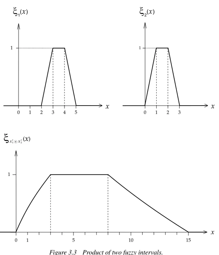
1⊙x2∗ of two fuzzy numbers with corresponding char-acterizing functions ξ1(·) and ξ2(·) is defined by using the extension principle to the function f :R2→Rwith f(x,y)=x·y, after combining x∗1 and x2∗ by the minimum t-norm.
The characterizing functionξx∗
1⊙x∗2(·) of thefuzzy product x
Remark 3.5:Using Theorem 3.1 theδ-cuts of the productx∗
1⊙x2∗can be calculated:
It can be proved that the following is valid:
LetCδ(x∗
It should be noted that the product of trapezoidal fuzzy numbers is not trapezoidal. In Figure 3.3 an example for the product of fuzzy numbers is given by using characterizing functions.
The special case of multiplication of a fuzzy number by a real constantc∈Ris calledscalar multiplicationof fuzzy numbers.
For fuzzy numbersx∗with characterizing functionξ(·) andc∈R\{0}, the mul-tiplicationc·x∗ yields a fuzzy number whose characterizing functionη(·) is given by
3.4
Mean value of fuzzy numbers
Arithmetic operations for fuzzy numbers can be extended to more than two fuzzy numbers by the associativity oft-norms.
26 STATISTICAL METHODS FOR FUZZY DATA
Figure 3.3 Product of two fuzzy intervals.
The sum ofnfuzzy numbersx∗
1, . . . ,x∗nis denoted by n
⊕
i=1x ∗
i =x
∗
1 ⊕x2∗⊕ · · · ⊕xn∗.
Combining this with scalar multiplication yields thearithmetic meanof fuzzy numbers:
1 n ·
n
⊕
i=1x ∗
i
MATHEMATICAL OPERATIONS FOR FUZZY QUANTITIES 27
Proposition 3.3:Letx∗1, . . . ,xn∗be fuzzy intervals withδ-cutsCδ(x∗
i)=[aδ,i;bδ,i],
then the fuzzy arithmetic mean
x∗n = 1
Proof:This is a consequence of Theorem 3.1.
Remark 3.6: The minimum t-norm is the only combination rule for which 1
3.5
Differences and quotients
The differencex∗
1⊖x2∗of two fuzzy numbersx1∗ andx2∗ are defined, using−x2∗:= (−1)·x∗
2, byx1∗⊖x2∗:=x1∗⊕(−x2∗). The quotientx∗
1 :x2∗is defined by the function f(x,y)=x/y, provided that 0∈/ supp (x∗
2).
3.6
Fuzzy valued functions
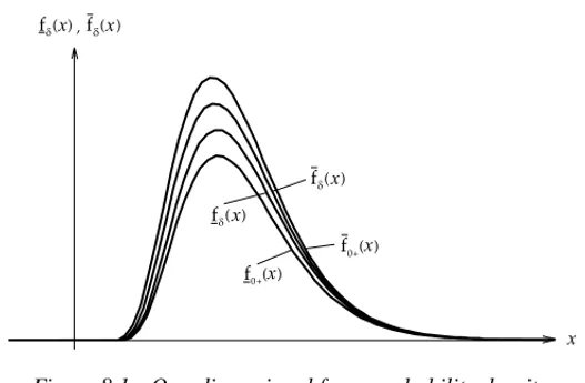
Fuzzy valued functions f∗(·) are functions whose range of values are fuzzy intervals, i.e.
for variablexthe real valued functions f
δ(·) and fδ(·) are calledδ-level functions. In the caseM =Rtheδ-level functions are calledδ-level curves.
Fuzzy valued functions can be graphically displayed by depicting someδ-level curves. An example is given in Figure 3.4.
28 STATISTICAL METHODS FOR FUZZY DATA
Figure 3.4 δ-Level curves of a fuzzy valued function.
Definition 3.3: Let f∗(·) be a fuzzy valued function defined on a measure space (M,A, µ). If allδ-level functions f
fδ(x)dµ(x),then the generalized integral
f∗(x)dµ(x) is the fuzzy numberJ∗whoseδ-cutsC
δ(J∗) are defined by
By the representation Lemma 2.1 the characterizing function of the fuzzy integral J∗is given by
fδ(x)dµ(x). The resulting fuzzy integral is
denoted by−
f∗(x)dµ(x).
Remark 3.8:For fuzzy valued real functions, i.e. f∗: [a,b]→FI(R) and integrable
δ-level curves thefuzzy integralis defined byJδ =
b
The resulting fuzzy value is denoted by−
b
a
f∗(x)d x.
3.7
Problems
MATHEMATICAL OPERATIONS FOR FUZZY QUANTITIES 29
(b) Prove the formula for theδ-cuts ofx1∗⊙x2∗in Remark 3.3 ifx1∗andx2∗are fuzzy intervals.
(c) Two fuzzy intervalsx1∗ andx∗
2 are given by their characterizing functions ξ1(·) andξ2(·):
Calculate and draw the characterizing function ofx1∗⊕x2∗.
(d) Calculate and draw the characterizing function of the productx1∗⊙x2∗forx1∗and x∗
2 in (c).
(e) Explain that the generalized integration of fuzzy valued functions reduces to the classical integration for classical real valued functions.
Part II
DESCRIPTIVE
STATISTICS FOR
FUZZY DATA
4
Fuzzy samples
Fuzzy samples consist of a finite sequence of fuzzy numbers, i.e. x∗
1, . . .xn∗, or a
finite sequence of fuzzy vectorsx∗
1, . . .x∗n. In this chapter the concepts of minimum
and maximum of observations are extended to fuzzy samples. Moreover generalized cumulative sums are introduced.
4.1
Minimum of fuzzy data
Let x∗
1, . . .xn∗ be n fuzzy intervals whose corresponding δ-cuts are denoted by
Cδ(x∗
i)=[xδ,i,xδ,i] for δ∈(0; 1] and i =1(1)n. The fuzzy valued minimum
min{x∗
1, . . .xn∗}is a fuzzy intervalxmin∗ whoseδ-cuts Cδ(x∗min) are defined by Cδ(x∗
min) :=
min
xδ,i:i=1(1)n
; min
xδ,i :i =1(1)n
∀δ∈(0; 1].
The characterizing function of x∗
min is obtained by (the representation) Lemma 2.1.
4.2
Maximum of fuzzy data
Under the same conditions as in Section 4.1 the maximum of n fuzzy intervals x∗
1, . . .xn∗ is the fuzzy interval xmax∗ =max{x1∗, . . .xn∗}whose δ-cuts Cδ(xmax∗ ) are defined by
Cδ(x∗
max)=
max
xδ,i :i =1(1)n
; max
xδ,i :i=1(1)n
∀δ∈(0; 1].
34 STATISTICAL METHODS FOR FUZZY DATA
Remark 4.1: The minimum as well as maximum of fuzzy intervals reduce to the classical minimum and maximum for classical samplesx1, . . . ,xn.
Examples are given in Section 4.4.
4.3
Cumulative sum for fuzzy data
In the case of classical samplesx1, . . . ,xnwithxi∈Rof one-dimensional quantities,
cumulative sums are defined by
#{xi:xi ≤x} ∀x ∈R,
and normalized cumulative sumsSn(·) are defined by
Sn(x) :=
#{xi:xi ≤x}
n ∀x∈R.
Such cumulative sums give the proportion of observations which are not larger than a given real valuex.
Remark 4.2:For (idealized) precise observationsxi ∈Rthe cumulative sum
coin-cides with theempirical distribution functionFˆn(·), defined by its values
∧
Fn(x) :=
1 n
n
i=1
I(−∞;x](xi) ∀x∈R.
For fuzzy observations given as fuzzy numbersxi∗,i=1(1)n, the definition of cumulative sums has to be adapted. Thisadapted cumulative sum Sad
n (·) is defined
using the characterizing functionsξi(·) ofxi∗,i =1(1)n, which are assumed to be
integrable, by
Snad(x) :=
n
i=1
x
−∞
ξi(t)dt n
i=1
∞
−∞
ξi(t)dt
∀x∈R.
Remark 4.3:Sad
n (x) is the proportion of fuzzy observations less than or equal tox.
4.4
Problems
(a) A fuzzy sample is given by its characterizing functionsξi(·),i=1(1)8, in the
FUZZY SAMPLES 35
Calculate and draw the resulting fuzzy minimum and fuzzy maximum of this fuzzy sample.
(b) Make a diagram for the adapted cumulative sum function Sad
n (·) for the fuzzy
5
Histograms for fuzzy data
Classical histograms are based on precise data x1, . . . ,xn in order to explain the
distribution of the observations xi. In order to construct histograms the set M
of possible values xi is decomposed into so-called classes K1, . . . ,Kk with Ki∩
Kj= ∅ ∀i = j, and
k
∪
j=1Kj =M.
Then for each classKj the so-calledrelative frequency hn(Kj) is calculated, i.e.
hn(Kj) :=
#
xi :xi ∈Kj
n , j =1(1)k.
The display of the relative frequencies is called a histogram.
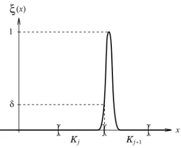
For fuzzy data the following problem arises: By the fuzziness of observations it is not always possible to decide in which class Kj a fuzzy observationx∗ with
characterizing functionξ(·) lies. This is depicted in Figure 5.1. Therefore a generalization of histograms is necessary.
5.1
Fuzzy frequency of a fixed class
Due to the possible inability to decide in which class a fuzzy data pointxi∗lies it seems natural to consider fuzzy values of relative frequencies. For n fuzzy observations x∗1, . . . ,xn∗and classes K1, . . . ,Kkthe fuzzy relative frequencies of the classes are
38 STATISTICAL METHODS FOR FUZZY DATA
Figure 5.1 Fuzzy observation and classes of a histogram.
denoted byh∗n(Kj), j=1(1)k. The characterizing function ofh∗n(Kj) is constructed
via itsδ-cuts
Cδ
h∗n Kj
=hn,δ(Kj);hn,δ(Kj)
,
where the limit pointshn,δ(Kj) andhn,δ(Kj) are defined in the following way:
hn,δ(Kj)=
#
x∗
i :Cδ(x
∗
i)∩Kj = ∅
n
and
hn,δ(Kj)=
#
x∗
i :Cδ(xi∗)⊆Kj
n
for allδ∈[0; 1].
The characterizing functionηj(·) ofh∗n(Kj) is obtained by Lemma 2.1.
Remark 5.1: The characterizing function of a fuzzy relative frequency is a step-function. In Figure 5.2 the characterizing functions of a sample of size 8 are given. In Figure 5.3 the characterizing function of the fuzzy relative frequency of the class [1; 2] is depicted.
5.2
Fuzzy frequency distributions
Considering all classes K1, . . . ,Kk of a decomposition of M, the fuzzy relative
frequencies h∗
n(Kj), j=1(1)k are defining a special fuzzy valued function f∗:
M →FI(R) from Section 3.6. For everyx ∈M the fuzzy value f∗(x) is defined in
the following way:
Determine the classKjwithx∈Kj, and define the fuzzy value
HISTOGRAMS FOR FUZZY DATA 39
Figure 5.2 Fuzzy sample.
Remark 5.2:The abstract mathematical model for idealized fuzzy histograms are so-calledfuzzy probability distributions, especially fuzzy probability densities which are described in Part III, and especially in Chapter 9.
Graphically fuzzy histograms can be depicted usingδ-level functions, andδ-level curves for one-dimensional distributions.
An alternative way of representing fuzzy histograms is given in the next section.
Remark 5.3:Different from histograms for precise data, where relative frequencies hn(·) are additive, i.e. for two disjoint setsAandBwe have
hn(A∪B)=hn(A)+hn(B),
for fuzzy relative frequencies h∗n(Kj) less restrictive relations for the boundaries
hn.δ(Kj) andhn,δ(Kj) of theδ-cuts are valid, i.e.
hn,δ
Ki∪Kj
≤hn,δ(Ki)+hn,δ(Kj) (5.1)
and
hn,δKi∪Kj
≥hn,δ(Ki)+hn,δ(Kj) (5.2)
for allδ∈(0; 1].
40 STATISTICAL METHODS FOR FUZZY DATA
Moreover the fuzzy relative frequencies of the extreme events∅andMare precise numbers, i.e.
h∗n(∅) has characterizing functionI{0}(·)
and
h∗n(M) has characterizing functionI{1}(·).
5.3
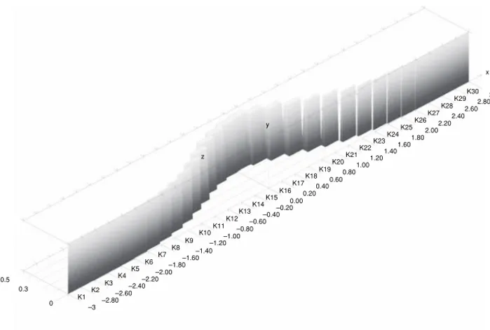
Axonometric diagram of the fuzzy histogram
For one-dimensional data the characterizing functions of the fuzzy relative fre-quencies are constant on the classes Kj. Therefore it is possible to depict them
in an axonometric way. One axis is the axis on which the classes are defined. The second axis is the independent variabley for the characterizing functionηj(·)
of the fuzzy relative frequency h∗
n(Kj). The third axis is the axis for the values
ηj(y).
An example of the axonometric picture of a fuzzy histogram is given in Figure 5.4.
HISTOGRAMS FOR FUZZY DATA 41
5.4
Problems
(a) For the fuzzy sample with characterizing functions given by the following diagram
0 1 2 3 4 5 6
0 1
use the classes K1=[0; 1], K2 =(1; 2], K3=(2; 3], . . . ,K10=(9; 10] and calculate the fuzzy relative frequenciesh∗15(Kj) for j =1(1)10.
6
Empirical distribution
functions
The classical empirical distribution function fornprecise data points x1, . . . ,xn is
defined by
ˆ Fn(x) :=
1 n
n
i=1
I(−∞;x](xi) for allx∈R.
6.1
Fuzzy valued empirical distribution function
For fuzzy samples x∗
1, . . . ,xn∗ with corresponding characterizing functions
ξ1(·), . . . , ξn(·) the counterpart to the empirical distribution function is a fuzzy valued
function ˆF∗
n(·) defined on Rwhose lower and upperδ-level functions ˆFδ,L(·) and
ˆ
Fδ,U(·) are defined via the δ-cuts Cδ(xi∗) of the fuzzy observationsx
∗
i, which are
assumed to be fuzzy intervals.
For fixedx ∈Rthe values ˆFδ,L(x) and ˆFδ,U(x) are defined by
ˆ
Fδ,U(x) :=
#
xi∗ :Cδ(x∗
i)∩(−∞;x]= ∅
n
ˆ
Fδ,L(x) :=
#
xi∗ :Cδ(x∗
i)⊆(−∞;x]
n
for allδ∈[0; 1].
44 STATISTICAL METHODS FOR FUZZY DATA
Lemma 6.1:For fuzzy intervalsx1∗, . . . ,xn∗whoseδ-cuts are given by Cδ(xi∗)=
xδ,i;xδ,i
∀δ∈(0; 1]
the correspondingδ-level functions of the fuzzy valued empirical distribution function are given by
ˆ
Fδ,U(x)=
1 n
n
i=1
I(−∞;x](xδ,i)
and
ˆ
Fδ,L(x)=
1 n
n
i=1
I(−∞;x](xδ,i),
respectively.
Proof: For the value ˆFδ,U(x) of the upper δ-level function ˆFδ,U(·) we have
Cδ(x∗
i)∩(−∞;x]= ∅ if and only if xδ,i ≤x, and this is equivalent to
I(−∞;x](xδ,i)=1.
Analogously for ˆFδ,L(x) we have Cδ(xi∗)⊆(−∞;x] if and only if xδ,i ≤x,
which is equivalent toI(−∞;x](xδ,i)=1.
In Figure 6.1 a fuzzy sample and the lower and upper δ-level curves of the corresponding fuzzy empirical distribution function are depicted.
Figure 6.1 Fuzzy sample and correspondingδ-level curves ofFˆ∗
EMPIRICAL DISTRIBUTION FUNCTIONS 45
Figure 6.2 Construction of Cδ(q∗
p).
6.2
Fuzzy empirical fractiles
For classical empirical distribution functions ˆFn(·) the empirical fractiles are defined
in the following way: Let p∈(0; 1) then thep-fractilexpis given by
min
x∈R: ˆFn(x)≥ p.
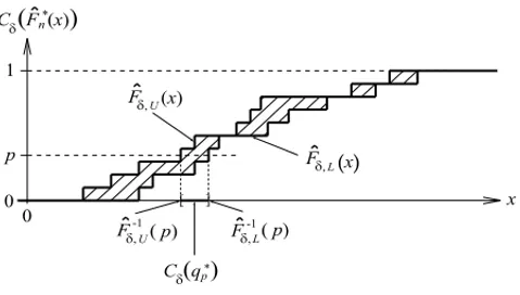
In the case of fuzzy empirical distribution functions ˆF∗
n(·) generalized empirical
fractiles are fuzzy numbers. The characterizing function or theδ-cuts of the fuzzy empirical fractiles are defined in the following way:
For p∈(0,1) the lower and upperδ-level curves ˆFδ,L(·) and ˆFδ,U(·) are used to
define theδ-cuts of the corresponding fuzzy fractileq∗
p. Theδ-cutCδ(q∗p) is defined
by
Cδ(q∗
p)=
ˆ
Fδ,−U1(p); ˆFδ,−L1(p)
∀δ ∈(0; 1).
The method is explained in Figure 6.2.
Remark 6.1:The characterizing functionξq∗
p(·) of the fuzzy empirical quantileq ∗
pis
obtained by Lemma 2.1.
6.3
Smoothed empirical distribution function
Another possibility to adapt the concept of the empirical distribution function to the situation of fuzzy data is the so-calledsmoothed empirical distribution function
ˆ Fnsm(·).
The values ˆFnsm(x) of the smoothed empirical distribution function based on fuzzy data x1∗, . . . ,x∗n with characterizing functionsξ1(·), . . . , ξn(·) are defined by
46 STATISTICAL METHODS FOR FUZZY DATA
(cf. Remark 4.2).
ˆ
Fnsm(x) := 1 n
n
i=1
x
−∞ ξi(t)dt
∞
−∞ ξi(t)dt
∀x∈R
provided that all characterizing functions ξ1(·), . . . , ξn(·) are integrable with finite
integral
∞
−∞
ξi(t)dt <∞.
In case the sample contains some precise values, say x1, . . . ,xl and the rest
are fuzzy values x∗
l+1, . . . ,xn∗ with characterizing functions ξl+1(·), . . . , ξn(·), the
smoothed empirical distribution function is defined by
ˆ
Fnsm(x) := 1 n
l
i=1
I(−∞;x](xi)+
1 n
n
i=l+1
x
−∞ ξi(t)dt
∞
−∞ ξi(t)dt
∀x∈R.
In Figure 6.3 a so-called mixed sample and the corresponding smoothed empirical distribution function are depicted.
EMPIRICAL DISTRIBUTION FUNCTIONS 47
6.4
Problems
(a) Use the fuzzy sample from Figure 6.1 and draw diagrams of the corresponding smoothed empirical distribution function as well as the corresponding adapted cumulative sum function.
7
Empirical correlation for
fuzzy data
For classical two-dimensional data (xi,yi)∈R2,i=1(1)nthe empirical correlation
coefficientris defined by
r:=
n
i=1
(xi−xn)(yi−yn)
n
i=1
(xi−xn)2
·
n
i=1
yi−yn
2
.
Remark 7.1:Forrthe following holds:
(a) −1≤r≤1.
(b) |r| =1 if and only if all points (xi,yi) are on a line in the (x,y)-plane.
7.1
Fuzzy empirical correlation coefficient
For real data fuzziness can be present in different ways:
(a) (xi,yi)∗can be fuzzy two-dimensional vectors.
(b) (x∗
i,yi∗) are pairs of fuzzy numbers.
(c) One coordinate is precise and the other is fuzzy.
In order to apply the extension principle for the generalization of the empirical correlation coefficient, first the fuzzy data have to be combined into a fuzzy vector of
50 STATISTICAL METHODS FOR FUZZY DATA
F
igur
e
7.1
Fuzzy
corr
elation
coef
EMPIRICAL CORRELATION FOR FUZZY DATA 51
F
igur
e
7.2
P
artially
fuzzy
data
and
corr
elation
coef
52 STATISTICAL METHODS FOR FUZZY DATA
the 2n-dimensional Euclidean spaceR2n. For this combination the minimum t-norm
is used.
In case (a) the fuzzy data consist of two-dimensional fuzzy vectors
x∗i, i =1(1)n
with corresponding vector-characterizing functionsξi(., .),i =1(1)n.
The combined fuzzy sample is a 2n-dimensional fuzzy vector whose vector-characterizing functionξ(., . . . , .) is given by its values
ξ(x1,y1, . . . ,xn,yn)=min{ξi(xi,yi) :i=1(1)n} ∀(x1,y1, . . . ,xn,yn)∈Rn.
Applying the extension principle to the function
(x1,y1, . . . ,xn,yn)→corr (x1,y1, . . . ,xn,yn)
=
n
i=1
(xi−xn)
yi−yn
n
i=1
(xi−xn)2
·
n
i=1
yi−yn
2
the characterizing function ψr∗(·) of the generalized (fuzzy) empirical correlation coefficientr* is given by its values
ψr∗(r) :=
sup{ξ(x1,y1, . . . ,xn,yn) : for corr (x1,y1, . . . ,xn,yn)=r}
0 otherwise
∀r∈R.
Remark 7.2:The support ofr* is a subset of the interval [−1; 1].
In Figure 7.1 an example of fuzzy two-dimensional data and the corresponding fuzzy correlation coefficient is depicted.
Cases (b) and (c) are treated in a similar way. The only difference is thatξi(., .)
have to be formed by applying the minimumt-norm also. The rest is analogous to case (a).
An example for this case is given in Figure 7.2.
7.2
Problems
(a) What shape has the characterizing function of the empirical correlation coefficient in the case of data in the form of two-dimensional intervals?
(b) Explain in detail how to obtain the vector-characterizing functionξ(., . . . , .) of the combined fuzzy sample if thex-coordinates in (x,y)∗