coordinated by
Christian Retoré
Volume 1
Application of Graph
Rewriting to Natural
Language Processing
First published 2018 in Great Britain and the United States by ISTE Ltd and John Wiley & Sons, Inc.
Apart from any fair dealing for the purposes of research or private study, or criticism or review, as permitted under the Copyright, Designs and Patents Act 1988, this publication may only be reproduced, stored or transmitted, in any form or by any means, with the prior permission in writing of the publishers, or in the case of reprographic reproduction in accordance with the terms and licenses issued by the CLA. Enquiries concerning reproduction outside these terms should be sent to the publishers at the undermentioned address:
ISTE Ltd John Wiley & Sons, Inc. 27-37 St George’s Road 111 River Street London SW19 4EU Hoboken, NJ 07030
UK USA
www.iste.co.uk www.wiley.com
© ISTE Ltd 2018
The rights of Guillaume Bonfante, Bruno Guillaume and Guy Perrier to be identified as the authors of this work have been asserted by them in accordance with the Copyright, Designs and Patents Act 1988. Library of Congress Control Number: 2018935039
British Library Cataloguing-in-Publication Data
Introduction . . . ix
Chapter 1. Programming with Graphs . . . 1
1.1. Creating a graph . . . 2
1.2. Feature structures . . . 5
1.3. Information searches . . . 6
1.3.1. Access to nodes . . . 7
1.3.2. Extracting edges . . . 7
1.4. Recreating an order . . . 9
1.5. Using patterns with the GREW library . . . 11
1.5.1. Pattern syntax . . . 13
1.5.2. Common pitfalls . . . 16
1.6. Graph rewriting . . . 20
1.6.1. Commands . . . 22
1.6.2. From rules to strategies . . . 24
1.6.3. Using lexicons . . . 29
1.6.4. Packages . . . 31
1.6.5. Common pitfalls . . . 32
Chapter 2. Dependency Syntax: Surface Structure and Deep Structure . . . 35
2.1. Dependencies versus constituents . . . 36
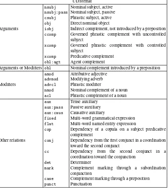
2.2. Surface syntax: different types of syntactic dependency . . . 42
2.2.1. Lexical word arguments. . . 44
2.2.3. Multiword expressions . . . 51
2.2.4. Coordination . . . 53
2.2.5. Direction of dependencies between functional and lexical words. . . 55
2.3. Deep syntax . . . 58
2.3.1. Example . . . 59
2.3.2. Subjects of infinitives, participles, coordinated verbs and adjectives . . . 61
2.3.3. Neutralization of diatheses . . . 61
2.3.4. Abstraction of focus and topicalization procedures . . . 64
2.3.5. Deletion of functional words . . . 66
2.3.6. Coordination in deep syntax . . . 68
Chapter 3. Graph Rewriting and Transformation of Syntactic Annotations in a Corpus . . . 71
3.1. Pattern matching in syntactically annotated corpora . . . 72
3.1.1. Corpus correction . . . 72
3.1.2. Searching for linguistic examples in a corpus. . . 77
3.2. From surface syntax to deep syntax . . . 79
3.2.1. Main steps in the SSQ_to_DSQ transformation . . . 80
3.2.2. Lessons in good practice . . . 83
3.2.3. TheUD_to_AUDtransformation system . . . 90
3.2.4. Evaluation of theSSQ_to_DSQandUD_to_AUD systems . . . 91
3.3. Conversion between surface syntax formats . . . 92
3.3.1. Differences between theSSQandUDannotation schemes . . . 92
3.3.2. TheSSQtoUDformat conversion system . . . 98
3.3.3. TheUDtoSSQformat conversion system . . . 100
Chapter 4. From Logic to Graphs for Semantic Representation . . . 103
4.1. First order logic . . . 104
4.1.1. Propositional logic. . . 104
4.1.2. Formula syntax inFOL . . . 106
4.1.3. Formula semantics inFOL . . . 107
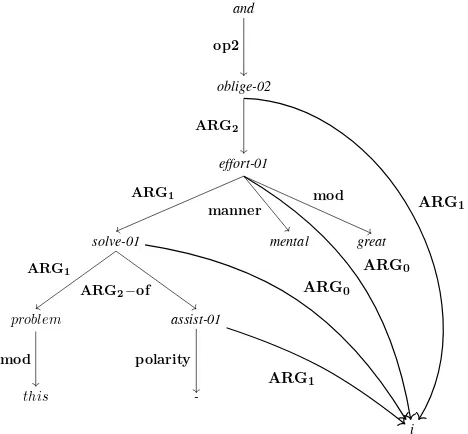
4.2. Abstract meaning representation (AMR) . . . 108
4.2.2. Examples of phenomena modeled usingAMR . . . 113
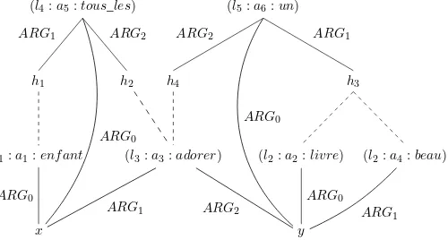
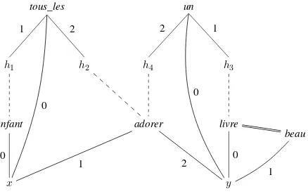
4.3. Minimal recursion semantics, MRS . . . 118
4.3.1. Relations between quantifier scopes . . . 118
4.3.2. Why use an underspecified semantic representation? . . . . 120
4.3.3. The RMRS formalism. . . 122
4.3.4. Examples of phenomenon modeling in MRS . . . 133
4.3.5. From RMRS to DMRS . . . 137
Chapter 5. Application of Graph Rewriting to Semantic Annotation in a Corpus . . . 143
5.1. Main stages in the transformation process. . . 144
5.1.1. Uniformization of deep syntax . . . 144
5.1.2. Determination of nodes in the semantic graph . . . 145
5.1.3. Central arguments of predicates . . . 147
5.1.4. Non-core arguments of predicates . . . 147
5.1.5. Final cleaning . . . 148
5.2. Limitations of the current system . . . 149
5.3. Lessons in good practice . . . 150
5.3.1. Decomposing packages . . . 150
5.3.2. Ordering packages. . . 151
5.4. The DSQ_to_DMRS conversion system . . . 154
5.4.1. Modifiers . . . 154
5.4.2. Determiners . . . 156
Chapter 6. Parsing Using Graph Rewriting . . . 159
6.1. The Cocke–Kasami–Younger parsing strategy . . . 160
6.1.1. Introductory example . . . 160
6.1.2. The parsing algorithm . . . 163
6.1.3. Start with non-ambiguous compositions . . . 164
6.1.4. Revising provisional choices once all information is available. . . 165
6.2. Reducing syntactic ambiguity . . . 169
6.2.1. Determining the subject of a verb . . . 170
6.2.2. Attaching complements found on the right of their governors . . . 172
6.2.3. Attaching other complements . . . 176
6.3. Description of the POS_to_SSQ rule system. . . 180
6.4. Evaluation of the parser . . . 185
Chapter 7. Graphs, Patterns and Rewriting . . . 187
7.1. Graphs . . . 189
7.2. Graph morphism . . . 192
7.3. Patterns . . . 195
7.3.1. Pattern decomposition in a graph . . . 198
7.4. Graph transformations. . . 198
7.4.1. Operations on graphs . . . 199
7.4.2. Command language . . . 200
7.5. Graph rewriting system . . . 202
7.5.1. Semantics of rewriting . . . 205
7.5.2. Rule uniformity . . . 206
7.6. Strategies . . . 206
Chapter 8. Analysis of Graph Rewriting . . . 209
8.1. Variations in rewriting . . . 212
8.1.1. Label changes . . . 213
8.1.2. Addition and deletion of edges . . . 214
8.1.3. Node deletion . . . 215
8.1.4. Global edge shifts . . . 215
8.2. What can and cannot be computed . . . 217
8.3. The problem of termination. . . 220
8.3.1. Node and edge weights . . . 221
8.3.2. Proof of the termination theorem. . . 224
8.4. Confluence and verification of confluence. . . 229
Appendix . . . 237
Bibliography . . . 241
Our purpose in this book is to show howgraph rewritingmay be used as a tool innatural language processing. We shall not propose any new linguistic theories to replace the former ones; instead, our aim is to present graph rewriting as a programming language shared by several existing linguistic models, and show that it may be used to represent their concepts and to transform representations into each other in a simple and pragmatic manner. Our approach is intended to include a degree of universality in the way computations are performed, rather than in terms of the object of computation. Heterogeneity is omnipresent in natural languages, as reflected in the linguistic theories described in this book, and is something which must be taken into account in our computation model.
Graph rewriting presents certain characteristics that, in our opinion, makes it particularly suitable for use in natural language processing.
Note, however, that in everyday language, notably spoken, it is easy to find occurrences of text which only partially respect established rules, if at all. For practical applications, we therefore need to consider language in a variety of forms, and to develop the ability to manage both rules and their real-world application with potential exceptions.
A second important remark with regard to natural language is that it involves a number of forms of ambiguity. Unlike programming languages, which are designed to be unambiguous and carry precise semantics, natural language includes ambiguities on all levels. These may be lexical, as in the phrase There’s a bat in the attic, where the bat may be a small nocturnal mammal or an item of sports equipment. They may be syntactic, as in the example “call me a cab”: does the speaker wish for a cab to be hailed for them, or for us to say “you’re a cab”? A further form of ambiguity is discursive: for example, in an anaphora, “She sings songs”, who is “she”?
In everyday usage by human speakers, ambiguities often pass unnoticed, as they are resolved by context or external knowledge. In the case of automatic processing, however, ambiguities are much more problematic. In our opinion, a good processing model should permit programmers to choose whether or not to resolve ambiguities, and at which point to do so; as in the case of constraint programming, all solutions should a priori be considered possible. The program, rather than the programmer, should be responsible for managing the coexistence of partial solutions.
I.1. Levels of analysis
A variety of linguistic theories exist, offering relatively different visions of natural language. One point that all of these theories have in common is the use of multiple, complementary levels of analysis, from the simplest to the most complex: from the phoneme in speech or the letter in writing to the word, sentence, text or discourse. Our aim here is to provide a model which is sufficiently generic to be compatible with these different levels of analysis and with the different linguistic choices encountered in each theory.
Although graph structures may be used to represent different dimensions of linguistic analysis, in this book, we shall focus essentially on syntax and semantics at sentence level. These two dimensions are unavoidable in terms of language processing, and will allow us to illustrate several aspects of graph rewriting. Furthermore, high-quality annotated corpora are available for use in validating our proposed systems, comparing computed data with reference data.
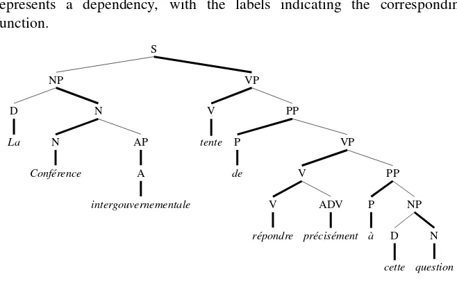
The purpose of syntax is to represent the structure of a sentence. At this level, lexical units – in practice, essentially what we refer to as words – form the basic building-blocks, and we consider the ways in which these blocks are put together to construct a sentence. There is no canonical way of representing these structures and they may be represented in a number of ways, generally falling into one of two types: syntagmatic or dependency-based representations.
These formalisms all feature more or less explicit elements of formal logic. For a simple transitive sentence, such asMax hates Luke, the two proper nouns are interpreted as constants, and the verb is interpreted as a predicate,H ate, for which the arguments are the two constants. Logical quantifiers may be used to account for certain determiners. The phrase“a man enters.”may thus be represented by the first-order logical formula∃x(M an(x)∧Enter(x)).
In what follows, we shall discuss a number of visions of syntax and semantics in greater detail, based on published formalisms and on examples drawn from corpora, which reflect current linguistic usage.
There are significant differences between syntactic and semantic structures, and the interface between the two levels is hard to model. Many linguistic models (including Mel’ˇcuk and Chomsky) feature an intermediary level between syntax, as described above, and semantics. This additional level is often referred to asdeep syntax.
To distinguish between syntax, as presented above, and deep syntax, the first is often referred to as surface syntax orsurface structure.
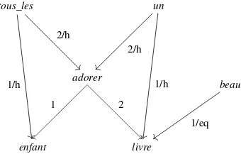
These aspects will be discussed in greater detail later. For now, note simply that deep structure represents the highest common denominator between different semantic representation formalisms. To avoid favoring any specific semantic formalism, deep structure uses the same labels as surface structure to describe new relations. For this reason, it may still be referred to as “syntax”. Deep structure may, for example, be used to identify new links between a predicate and one of its semantic arguments, which cannot be seen from the surface, to neutralize changes in verb voice (diathesis) or to identify grammatical words, which do not feature in a semantic representation. Deep structure thus ignores certain details that are not relevant in terms of semantics. The following figure is an illustration of a passive voice, with the surface structure shown above and the deep structure shown below, for the French sentence “Un livre est donné à Marie par Luc” (A book is given to Mary by Luc).
I.2. Trees or graphs?
The notion of trees has come to be used as the underlying mathematical structure for syntax, following Chomsky and the idea of syntagmatic structures. The tree representation is a natural result of the recursive process by which a component is described from its direct subcomponents. In dependency representations, as introduced by Tesnière, linguistic information is expressed as binary relations between atomic lexical units. These units may be considered as nodes, and the binary relations as arcs between the nodes, thus forming a graph. In a slightly less direct manner, dependencies are also governed by a syntagmatic vision of syntax, naturally leading to the exclusion of all dependency structures, which do not follow a tree pattern. In practice, in most corpora and tools, dependency relations are organized in such a way that one word in a sentence is considered as the root of the structure, with each other node as the target of one, and only one, relation. The structure is then a tree.
This book is intended to promote a systematic and unified usage of graph representations. Trees are considered to facilitate processing and to simplify analytical algorithms. However, the grounds for this argument are not particularly solid, and, as we shall see through a number of experiments, the processing cost of graphs, in practice, is acceptable. Furthermore, the tools presented in what follows have been designed to permit use with a tree representation at no extra cost.
While the exclusive use of tree structures may seem permissible in the field of syntactic structures, it is much more problematic on other levels, notably for semantic structures. A single entity may play a role for different predicates at the same time, and thus becomes the target of a relation for each of these roles. At the very least, this results in the creation of acylic graphs; in practice, it means that a graph is almost always produced. The existing formalisms for semantics, which we have chosen to present below (AMR and DMRS), thus make full use of graph structures.
structure and the linear order of words). Note that, in practice, tree-based formalisms often include ad hoc mechanisms, such as coindexing, to represent relations, which lie outside of the tree structure. Graphs allow us to treat these mechanisms in a uniform manner.
I.3. Linguistically annotated corpora
Whilst the introspective work carried out by lexicographers and linguists is often essential for the creation of dictionaries and grammars (inventories of rules) via the study of linguistic constructs, their usage and their limitations, it is not always sufficient. Large-scale corpora may be used as a means of considering other aspects of linguistics. In linguistic terms, corpus-based research enables us to observe the usage frequency of certain constructions and to study variations in language in accordance with a variety of parameters: geographic, historical or in terms of the type of text in question (literature, journalism, technical text, etc.). As we have seen, language use does not always obey those rules described by linguists. Even if a construction or usage found in a corpus is considered to be incorrect, it must be taken into account in the context of applications.
Linguistic approaches based on artificial intelligence and, more generally, on probabilities, use observational corpora for their learning phase. These corpora are also used as references for tool validation.
Raw corpora (collections of text) may be used to carry out a number of tasks, described above. However, for many applications, and for more complex linguistic research tasks, this raw text is not sufficient, and additional linguistic information is required; in this case, we use annotated corpora. The creation of these corpora is a tedious and time-consuming process. We intend to address this issue in this book, notably by proposing tools both for preparing (pre-annotating) corpora and for maintaining and correcting existing corpora. One solution often used to create annotated resources according to precise linguistic choices is to transform pre-existing resources, in the most automatic way possible. Most of the corpora used in the universal dependencies (UD) project1are corpora which had already been annotated in
the context of other projects, converted into UD format. We shall consider this type of application in greater detail later.
I.4. Graph rewriting
Our purpose here is to show how graph rewriting may be used as a model for natural language processing. The principle at the heart of rewriting is to break down transformations into a series of elementary transformations, which are easier to describe and to control. More specifically, rewriting consists of executing rules, i.e. (1) using patterns to describe the local application conditions of an elementary transformation and (2) using local commands to describe the transformation of the graph.
One of the ideas behind this theory is that transformations are described based on a linguistic analysis that, as we have seen, is highly suited to local analysis approaches. Additionally, rewriting is not dependent on the formalism used, and can successfully manage several coexisting linguistic levels. Typically, it may be applied to composite graphs, made up of heterogeneous links (for example those which are both syntactic and semantic). Furthermore, rewriting does not impose the order, nor the location, in which rules are applied. In practice, this means that programmers no longer need to consider algorithm design and planning, freeing them to focus on the linguistic aspects of the problem in question. A fourth point to note is that the computation model is intrinsically non-deterministic; two “contradictory” rules may be applied to the same location in the same graph. This phenomenon occurs in cases of linguistic ambiguity (whether lexical, syntactic or semantic) where two options are available (in the phrasehe sees the girl with the telescope, who has thetelescope?), each corresponding to a rule. Based on a strategy, the programmer may choose to continue processing using both possibilities, or to prefer one option over the other.
We shall discuss the graph rewriting formalism used in detail later, but for now, we shall simply outline its main characteristics. Following standard usage in rewriting, the “left part” of the rule describes the conditions of application, while the “right part” describes the effect of the rule on the host structure.
applied. The left part can also include rule parameters in the form of external lexical information. Graph pattern recognition is an NP-complete problem and, as such, is potentially difficult for practical applications; however, this is not an issue in this specific case, as the patterns are small (rarely more than five nodes) and the searches are carried out in graphs of a few dozen (or, at most, a few hundred) nodes. Moreover, patterns often present a tree structure, in which case searches are extremely efficient.
The right part of rules includes atomic commands (edge creation, edge deletion) that describe transformations applied to the graph at local level. There are also more global commands (shift) that allow us to manage connections between an identified pattern and the rest of the graph. There are limitations in terms of the creation of new nodes: commands exist for this purpose, but new nodes have a specific status. Most systems work without creating new nodes, a fact which may be exploited in improving the efficiency of rewriting.
Global transformations may involve a large number of intermediary steps, described by a large number of rules (several hundred in the examples presented later). We therefore need to control the way in which rules are applied during transformations. To do this, the set of rules for a system is organized in a modular fashion, featuring packages, for grouping coherent sub-sets of rules, and strategies, which describe the order and way of applying rules.
Here, we shall provide a more operational presentation of rewriting and rules, focusing on language suitable for natural language processing. We have identified a number of key elements to bear in mind in relation to this subject:
– negative conditions are essential to avoid over-interpretation;
– modules/packages are also necessary, as without them, the process of designing rewriting systems becomes inextricable;
– we need a strong link to lexicons, otherwise thousands of rules may come into play, making rewriting difficult to design and ineffective;
– a notion of strategy is required for the sequential organization of modules and the resolution of ambiguities.
The work presented in this book was carried out using GREW, a generic graph rewriting tool that responds to the requirements listed above. We used this tool to create systems of rules for each of the applications described later in the book. Other tools can be found in the literature, along with a few descriptions of graph rewriting used in the context of language processing (e.g. [HYV 84, BOH 01, CRO 05, JIJ 07, BÉD 09, CHA 10]). However, to the best of our knowledge, widely-used generic graph rewriting systems, with the capacity to operate on several levels of language description, are few and far between (the Ogre system is a notable exception [RIB 12]). A system of this type will be proposed here, with a description of a wide range of possible applications of this approach for language processing.
I.5. Practical issues
Whilst natural language may be manifested both orally and in writing, speech poses a number of specific problems (such as signal processing, disfluence and phonetic ambiguity), which will not be discussed here; for simplicity’s sake, we have chosen to focus on written language.
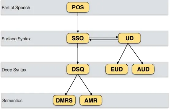
Our aim here is to study ways of programming conversions between formats. These transformations may take place within a linguistic level (shown by the horizontal arrows on the diagram) and permit automatic conversion of data between different linguistic descriptions on that level. They may also operate between levels (descending arrows in the diagram), acting as automatic syntactic or semantic analysis tools2. These different transformations will be discussed in detail later.
Part of Speech
Surface Syntax
Semantics
Deep Syntax DSQ
SSQ
DMRS AMR
EUD AUD
UD POS
Figure I.1.Formats and rewriting systems considered in this book
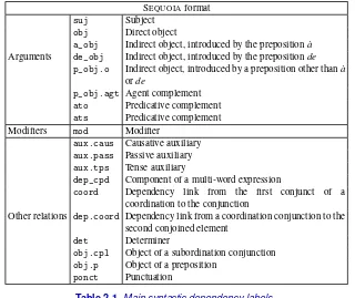
Our tools and methods have been tested using two freely available corpora, annotated using dependency syntax and made up of text in French. The first corpus is SEQUOIA3, made up of 3099 sentences from a variety of
domains: the press (theannodis_ersubcorpus), texts issued by the European parliament (the Europar.550 sub-corpus), medical notices (the emea-fr-dev and emea-fr-test subcorpora), and French Wikipedia (the frwiki_50.1000 sub-corpus). It was originally annotated using constituents, following the French Treebank annotation scheme (FTB) [ABE 04]. It was then converted
2 We have yet to attempt transformations in the opposite direction (upward arrows); this would be useful for text generation.
automatically into a surface dependency form [CAN 12b], with long-distance dependencies corrected by hand [CAN 12a]. Finally, SEQUOIAwas annotated
in deep dependency form [CAN 14]. Although the FTB annotation scheme used here predates SEQUOIAby a number of years, we shall refer to it as the
SEQUOIA format here, as we have only used it in conjunction with the
SEQUOIAcorpus.
The second corpus used here is part of the Universal Dependencies project4(UD). The aim of the UD project is to define a common annotation scheme for as many languages as possible, and to coordinate the creation of a set of corpora for these languages. This is no easy task, as the annotation schemes used in existing corpora tend to be language specific. The general annotation guide for UD specifies a certain number of choices that corpus developers must follow and complete for their particular language. In practice, this general guide is not yet set in stone and is still subject to discussion. The UD_FRENCHcorpus is one of the French-language corpora
in UD. It is made up of around 16000 phrases drawn from different types of texts (blog posts, news articles, consumer reviews and Wikipedia). It was annotated within the context of the Google DataSet project [MCD 13] with purely manual data validation. The annotations were then converted automatically for integration into the UD project (UD version 1.0, January 2015). Five new versions have since been issued, most recently version 2.0 (March 2017). Each version has come with new verifications, corrections and enrichments, many thanks to the use of the tools presented in this book. However, the current corpus has yet to be subject to systematic manual validation.
I.6. Plan of the book
Chapter 1 of this book provides a practical presentation of the notions used throughout. Readers may wish to familiarize themselves with graph handling inPYTHONand with the use ofGREWto express rewriting rules and the graph
transformations, which will be discussed later. The following four chapters alternate between linguistic presentations, describing the levels of analysis in question and examples of application. Chapter 2 is devoted to syntax (distinguishing between surface syntax and deep structure), while Chapter 4
focuses on the issue of semantic representation (via two proposed semantic formalization frameworks, AMR and DMRS). Each of these chapters is followed by an example of application to graph rewriting systems, working with the linguistic frameworks in question. Thus, Chapter 3 concerns the application of rewriting to transforming syntactic annotations, and Chapter 5 covers the use of rewriting in computing semantic representations. In Chapter 6, we shall return to syntax, specifically syntactic analysis through graph rewriting; although the aim in this case is complementary to that found in Chapter 3, the system in question is more complex, and we thus thought it best to devote a separate chapter to the subject. The last two chapters constitute a review of the notions presented previously, including rigorous mathematical definitions, in Chapter 7, designed for use in studying the properties of the calculation model presented in Chapter 8, notably with regard to termination and confluence. Most chapters also include exercises and sections devoted to “good practice”. We hope that these elements will be of use to the reader in gaining a fuller understanding of the notions and tools in question, enabling them to be used for a wide variety of purposes.
The work presented here is the fruit of several years of collaborative work by the three authors. It would be hard to specify precisely which author is responsible for contributions, the three played complementary roles. Guillaume Bonfante provided the basis for the mathematical elements, notably the contents of the final two chapters. Bruno Guillaume is the developer behind the GREW tool, while Guy Perrier developed most of the
rewriting systems described in the book, and contributed to the chapters describing these systems, along with the linguistic aspects of the book. The authors wish to thank Mathieu Morey for his participation in the early stages of work on this subject [MOR 11], alongside Marie Candito and Djamé Seddah, with whom they worked [CAN 14, CAN 17].
Programming with Graphs
In this chapter, we shall discuss elements of programming for graphs. Our work is based on PYTHON, a language widely used for natural language processing, as in the case of the NLTK library1(Natural Language ToolKit), used in our work. However, the elements presented here can easily be translated into another language. Several different data structures may be used to manage graphs. We chose to use dictionaries; this structure is elementary (i.e. unencapsulated), reasonably efficient and extensible. For what follows, we recommend opening an interactivePYTHONsession2.
Notes for advanced programmers: by choosing such a primitive structure, we do not have the option to use sophisticated error management mechanisms. There is no domain (or type) verification, no identifier verification, etc. Generally speaking, we shall restrict ourselves to the bare minimum in this area for reasons of time and space. Furthermore, we have chosen not to use encapsulation so that the structure remains as transparent as possible. Defining a class for graphs should make it easier to implement major projects. Readers are encouraged to take a more rigorous approach to that presented here after reading the book. Finally, note that the algorithms used here are not always optimal; once again, our primary aim is to improve readability.
1 http://www.nltk.org
2 Our presentation is inPYTHON3, butPYTHON2 can be used almost as-is.
Application of Graph Rewriting to Natural Language Processing, First Edition. Guillaume Bonfante, Bruno Guillaume and Guy Perrier.
Notes for “beginner” programmers: this book is not intended as an introduction toPYTHON, and we presume that readers have some knowledge of the language, specifically with regard to the use of lists, dictionaries and sets.
The question will be approached from a mathematical perspective in Chapter 7, but for now, we shall simply make use of an intuitive definition of graphs. A graph is a set of nodes connected by labeled edges. The nodes are also labeled (with a phonological form, a feature structure, a logical predicate, etc.). The examples of graphs used in this chapter are dependency structures, which simply connect words in a sentence using syntactic functions. The nodes in these graphs are words (W1,W2, . . . ,W5 in the example below), the
edges are links (suj, obj, det) and the labels on the nodes provide the phonology associated with each node. We shall consider the linguistic aspects of dependency structures in Chapter 2.
Note that it is important to distinguish between nodes and their labels. This enables us to differentiate between the two occurrences of"the"in the graph above, corresponding to the two nodesW1andW4.
In what follows, the nodes in the figures will not be named for ease of reading, but they can be found in the code in the form of strings :'W1','W2', etc.
1.1. Creating a graph
A graph is represented using a dictionary. Let us start with a graph with no nodes or edges.
✞ ☎
g = dict()
✝ ✆
The nodes are dictionary keys. The value corresponding to keyvis a pair
✞ ☎
g[' W1 '] = (' the ', [ ])
✝ ✆
Now, add a second and a third node, with the edges that connect them:
✞ ☎
g[' W2 '] = (' child ', [ ]) g[' W3 '] = (' plays ', [ ])
g[' W3 '] [1].append((' suj ', ' W2 ') ) g[' W2 '] [1].append((' det ', ' W1 ') )
✝ ✆
and print the result:
✞ ☎
g
✝ ✆
{' W1 ': (' the ', [ ]) , ' W2 ': (' child ', [(' det ', ' W1 ')]) , ' W3 ':
(' plays ', [(' suj ', ' W2 ')])}
The last box shows the output from the PYTHON interpreter. This graph is represented in the following form:
Let us return to the list of successors of a node. This is given in the form of a list of pairs(e, t), indicating the labeleof the edge and the identifiert
of the target node. In our example, the list of successors of node'W2'is given byg['W2'][1]. It contains a single pair('det', 'W1')indicating that the node'W1'corresponding to"the"is the determiner of'W2', i.e. the common noun"child".
In practice, it is easier to use construction functions:
✞ ☎
def a d d _ n o d e (g , u , a ):
# Add a node u labeled a in graph g g[u] = (a , [ ])
def a d d _ e d g e (g , u , e , v ):
# Add an edge labeled e from u to v in graph g
if (e , v ) not in g[u] [1] :
g[u] [1].append( (e , v ) )
This may be used as follows:
✞ ☎
a d d _ n o d e (g , ' W4 ', ' the ') a d d _ n o d e (g , ' W5 ', ' fool ') a d d _ e d g e (g , ' W3 ', ' obj ', ' W5 ') a d d _ e d g e (g , ' W5 ', ' det ', ' W4 ')
✝ ✆
to construct the dependency structure of the sentence"the child plays the fool":
Let us end with the segmentation of a sentence into words. This is represented as aflatgraph, connecting words in their order; we add an edge,
'SUC', between each word and its successor. Thus, for the sentence "She takes a glass", we obtain:
The following solution integrates theNLTKsegmenter:
✞ ☎
import nltk
w o r d _ l i s t = nltk . w o r d _ t o k e n i z e (" She takes a glass ") w o r d _ g r a p h = dict()
for i in range(len( w o r d _ l i s t ) ):
add_node ( word_graph , 'W%s ' % i , w o r d _ l i s t[i])
for i in range(len( w o r d _ l i s t ) - 1 ):
add_edge ( word_graph , 'W%s ' % i , ' SUC ', 'W%s ' % ( i + 1 ) ) w o r d _ g r a p h
✝ ✆
{' W3 ': (' glass ', [ ]) , ' W1 ': (' takes ', [(' SUC ', ' W2 ')]) , ' W2 ': ('a ', [(' SUC ', ' W3 ')]) , ' W0 ': (' She ', [(' SUC ', ' W1 ')])}
Readers may wish to practice using the two exercises as follows.
EXERCISE1.2.–Write a function to compute a graph in which all of the edges have been reversed. For example, we go from the dependency structure of "the child plays the fool"to:
1.2. Feature structures
So far, node labels have been limited to their phonological form, i.e. a string of characters. Richer forms of structure, namely feature structures, may be required. Once again, we shall use a dictionary:
✞ ☎
f s _ p l a y s = {' phon ' : ' plays ', ' cat ' : 'V '}
✝ ✆
Thefs_playsdictionary designates a feature structure with two features,
'phon' and 'cat', with respective values 'plays' and 'V'. To find the category'cat'of the feature structurefs_plays, we apply:
✞ ☎
f s _ p l a y s[' cat ']
✝ ✆
V
Let us reconstruct our initial sentence, taking account of feature structures:
✞ ☎
g = dict()
a d d _ n o d e (g , ' W1 ', {' phon ' : ' the ', ' cat ' : ' DET '} ) a d d _ n o d e (g , ' W2 ', {' phon ' : ' child ', ' cat ' : 'N '} ) a d d _ n o d e (g , ' W3 ', {' phon ' : ' plays ', ' cat ' : 'V '} ) a d d _ n o d e (g , ' W4 ', {' phon ' : ' the ', ' cat ' : ' DET '}) a d d _ n o d e (g , ' W5 ', {' phon ' : ' fool ', ' cat ' : 'N '}) a d d _ e d g e (g , ' W2 ', ' det ', ' W1 ')
a d d _ e d g e (g , ' W3 ', ' suj ', ' W2 ') a d d _ e d g e (g , ' W3 ', ' obj ', ' W5 ') a d d _ e d g e (g , ' W5 ', ' det ', ' W4 ')
The corresponding graph representation3is:
The “Part Of Speech” (POS) labeling found inNLTK4may also be used to construct a richer graph. The following solution shows how this labeling may be integrated in the form of a dictionary.
✞ ☎
import nltk
w o r d _ l i s t = nltk . w o r d _ t o k e n i z e (" She takes a glass ") t a g _ l i s t = nltk . pos_tag ( w o r d _ l i s t )
f e a t _ l i s t = [ {' phon ':n[0], ' cat ':n[1] } for n in t a g _ l i s t]
t_graph = {'W%s ' % i : ( f e a t _ l i s t[i], [ ])
for i in range(len( t a g _ l i s t ) )} for i in range(len( t a g _ l i s t )-1 ):
a d d _ e d g e ( t_graph , 'W%s ' % i , ' SUC ', 'W%s ' % ( i+1 ) ) t_graph
✝ ✆
{' W3 ': ({' phon ': ' glass ', ' cat ': ' NN '}, [ ]) , ' W1 ': ({' phon '
:
' takes ', ' cat ': ' VBZ '}, [(' SUC ', ' W2 ')]) , ' W2 ': ({' phon ':
'a ', ' cat ': ' DT '}, [(' SUC ', ' W3 ')]) , ' W0 ': ({' phon ': ' She ', ' cat ': ' PRP '}, [(' SUC ', ' W1 ')])}
1.3. Information searches
To find the label or feature structure of a node, we use:
✞ ☎
g[' W4 '] [0]
✝ ✆
{' phon ': ' the ', ' cat ': ' DET '}
or the function:
✞ ☎
def g e t _ l a b e l (g , u ): return g[u] [0]
✝ ✆
3 The feature namesphonandcatare not shown, as these are always present in applications. Other features are noted, for examplenum=sing.
The list of successors of a node is obtained using:
✞ ☎
def g e t _ s u c s (g , u ): return g[u] [1]
✝ ✆
1.3.1. Access to nodes
To find a list of nodes with a given property, we may begin by retrieving the list5of node identifiers:
✞ ☎
nodes = g . keys ()
✝ ✆
We then extract those which are of interest. For example, if we want a list of verbs:
✞ ☎
verbs = [ ] for u in nodes:
if g e t _ l a b e l (g , u )[' cat '] = = 'V ':
verbs .append( u )
✝ ✆
or, in a more compact manner with comprehension,
✞ ☎
verbs = [ u for u in g if g e t _ l a b e l (g , u )[' cat '] = = 'V ' ]
✝ ✆
You may wish to practice using the exercises as follows:
EXERCISE 1.3.–Find the list of node identifiers corresponding to the word
"the"in the graph of "the child plays the fool".
EXERCISE 1.4.–How can we find out if the same word occurs twice in a graph?
1.3.2. Extracting edges
The examples above relate to nodes. For edges, we begin by creating a list in the form of triplets(s, e, t)for each edge fromstotlabelede. We use a comprehension:
✞ ☎
t r i p l e t s = [ (s , e , t ) for s in g for (e , t ) in g e t _ s u c s (g , s ) ]
✝ ✆
or, more prosaically, loops:
✞ ☎
t r i p l e t s = [ ] for s in g:
for (e , t ) in g e t _ s u c s (g , s ):
t r i p l e t s .append( (s , e , t ) )
✝ ✆
From this, we can extract the pairs of nodes linked by a subject by selecting triplets of the form(v, 'suj', s), or, graphically:
✞ ☎
s u b j e c t _ v e r b s = [ (s , v ) for (v , e , s ) in t r i p l e t s if e= =' suj ' ]
✝ ✆
The triplet list is very practical, allowing us to find out whether any given nodesis linked totby a labele. We use:
✞ ☎
(s , e , t ) in t r i p l e t s
✝ ✆
More generally, the list enables us to respond to questions relating to the form of the graph. For example, to find out if there is an edge between two nodesuandv, we use the function:
✞ ☎
def a r e _ r e l a t e d (g , u , v ):
t r i p l e t s = [(s , e , t ) for s in g for (e , t ) in g e t _ s u c s (g , s )]
for (s , e , t ) in t r i p l e t s: if (s , t ) = = (u , v ):
return True return False
✝ ✆
✞ ☎ def is_root (g , u ):
t r i p l e t s = [(s , e , t ) for s in g for (e , t ) in g e t _ s u c s (g , s )]
for (s , e , t ) in t r i p l e t s: if t = = u:
return False return True
✝ ✆
EXERCISE 1.5.–Rewrite the functions are_related and is_root without using triplets.
EXERCISE 1.6.–A node is known as a leaf if it has no children. Write a function to find out whether a node in a graph is a leaf. Define a function with the profile:def is_leaf(g, u).
EXERCISE 1.7.–Write a function to select node triplets (s, v, o)
corresponding to the subject-verb-object configuration:
EXERCISE1.8.–A graph is said to be linear if it has a root node that only has one child, which only has one child, and so on up to a leaf node. An example can be found in exercise 1.1. Write a function to show if a graph is linear.
1.4. Recreating an order
Mathematically speaking, nodes are not, a priori, arranged in any order. For the dependency structure of the sentence "the child plays the fool", for example, the graph does not show that the word"child" precedes the word
"plays". The edges do not provide an order, and sometimes go “backward”, as in the case of determiner connections, or “forward”, as with the “obj” link in our example.
syntactic dependency structures (all nodes ordered), semantic structures (no nodes ordered) and syntagmatic structures (only leaf nodes are ordered).
For practical reasons, we have adopted the convention whereby identifiers starting with the letter “W” and followed by a number correspond to ordered nodes; the order is implicitly described by this number. Any other nodes are not ordered. Thus,'W1'comes before'W2'and'W2'precedes'W15'(even if the lexicographical order of the strings places'W15'before'W2'), but'S1'is not considered to be before'W2', nor is'W1'before'S2', nor'S1'before'S2'. Real values (with no exponential notation) are permitted, meaning that it is always possible to insert a new node, e.g.'W2.5', between two existing nodes, e.g.'W2'and'W3'. Using this convention, we can reconstruct the sentence corresponding to a graph using the following function:
✞ ☎
def g e t _ p h o n o l o g y ( g ):
def get_idx ( node ): # gets the float after 'W ' in node if any
import re # for r e g u l a r e x p r e s s i o n s
word_id = re . search (r 'W (\ d+(\.\ d+) ?) ', node )
return word_id . group ( 1 ) if word_id else None
words = {get_idx ( node ) : g e t _ l a b e l (g , node )[' phon '] for node in g if get_idx ( node )} return ' '. join ([ words[idx] for idx in sorted( words )]) g e t _ p h o n o l o g y ( g )
✝ ✆
the child plays the fool
Word order could be represented in a graph by adding'SUC'edges between consecutive nodes, as in the case of the flat graph. However, this choice comes at a cost. First, the graph does not tell us if a word is located at any given distance before another without computations. To obtain this information, we need to add elements to the graph, as in exercise 1.1, which results in a non-negligible increase in graph size: the equivalent full graph for a flat graph with
n−1edges will haven×(n−1)/2edges. In other words, the increase in graph size has a cost in terms of efficiency when searching for patterns. Second, if we begin to transform the graph in question, the order structure may be lost, and the programmer must constantly check for integrity.
way that is compatible with the order of the words themselves (alphabetical order). The exercise may also be carried out without this presumption, supposing each node to be connected to its successor by a'SUC'connection, as in the following example:
1.5. Using patterns with the GREW library
As we have seen in the previous examples, it is possible to select nodes within a graph that verify certain properties, such as belonging to the verb category, being connected by a certain link to another node; not being connected to another node, or coming before or after another given node in a sentence.
This type of property may be described using a pattern, which can be searched for among the nodes and edges of a graph.
The GREWlibrary features a syntax for describing patterns and offers the corresponding matching function. Separating the pattern matching code from the patterns themselves means that programming is much easier: usingGREW, programmers define their own patterns, which they can then modify without changing a single line of code. This is a significant advantage both in terms of design and long-term maintenance. Let us now consider the use of the library in practice.
GREW offers a dedicated syntax to facilitate graph handling, notably in terms of feature structures. The dependency structure of the sentence "the child plays the fool"can be constructed directly using the syntax:
✞ ☎
g = grew . graph (''' graph{
W2 - [det] - >W1 ; W3 - [suj] - >W2 ; W3 - [obj] - >W5 ; W5 - [det] - >W4 ;
}''')
✝ ✆
GREW also provides syntax for graph pattern matching. In the example below, we wish to find verbs; in other terms, we are searching for a nodeX
containing a featurecatof typeV:
✞ ☎
grew . search (" pattern { X [cat=V] }", g )
✝ ✆
[ {'X ': ' W3 '} ]
The result is presented in the form of a list of solutions (one, in this case) giving the link between nodes in the pattern and those in the graph in dictionary form. Hence, ifm denotes the output list, m[0]['X']denotes the node corresponding to'X'ing, in this case'W3'. Clearly, it is also possible to obtain multiple solutions, or, for that matter, none at all:
✞ ☎
grew . search (" pattern { X [cat=DET] }", g )
✝ ✆
[ {'X ': ' W4 '}, {'X ': ' W1 '} ]
✞ ☎
grew . search (" pattern { X [cat=ADJ] }", g )
✝ ✆
[ ]
Returning to our example from the previous section, let us search for asuj
type edge originating from a verb. This corresponds to searching for a pattern containing two nodes,XandY, connected by asuj link, where nodeX has a featurecatthat is equal toV. InPYTHON:
✞ ☎
grew . search (" pattern { X[cat=V]; Y[ ]; X - [suj] - > Y }", g )
✝ ✆
[ {'Y ': ' W2 ', ' __e_6__ ': ' W3 / suj / W2 ', 'X ': ' W3 '} ]
We obtain a dictionary associatingXwithW3andYwithW2. Furthermore, the system names the edges, assigning identifiers of the form__e_i__with an automatically generated indexi. In our example, this is the case for the edge
Nodes free from any constraint may be omitted. This is the case forYin the previous search, which may thus be simplified as follows:
✞ ☎
grew . search (" pattern { X[cat=V]; X - [suj] - > Y }", g )
✝ ✆
[ {' __e_8__ ': ' W3 / suj / W2 ', 'Y ': ' W2 ', 'X ': ' W3 '} ]
Edges can be named by the user. The request thus takes the form:
✞ ☎
grew . search (" pattern { X[cat=V]; e:X - [suj] - > Y }", g )
✝ ✆
[ {'Y ': ' W2 ', 'e ': ' W3 / suj / W2 ', 'X ': ' W3 '} ]
Finally, let us search for a root in the graph, i.e. a nodeX with no parents. We calculate:
✞ ☎
grew . search (" pattern { X[ ] } without { * - >X }", g )
✝ ✆
[ {'X ': ' W3 '} ]
Thewithoutkeyword indicates the part which must not be present in the graph – in this case, an edge towardX. The notation*denotes an anonymous node that cannot be referenced later.
1.5.1. Pattern syntax
Following on from this overview, we shall now consider the syntax of
GREWin greater detail. Broadly speaking, a pattern is described by a positive
element (that must be present in the graph) and a list of negative constraints (things that should not be present). The positive part of the pattern is represented by the keyword pattern, while negative constraints are represented by without. Each part is made up of a list of clauses. In short, the declaration of a pattern with a negative element takes the form:
pattern {
C_1; ... ; C_k; }
without {
where C_1, . . . , C_k, C'_1, . . . , C'_m are clauses. There are three types of clauses: node declarations, edge declarations and additional pattern constraints. These will be described in detail below.
1.5.1.1. Nodes
The following example illustrates the general syntax for a node declaration.
N [cat=V, m=ind|subj, t<>fut, n=*, !p, lemma="être"];
This declaration describes a node, named N, with a feature structure verifying the following conditions: it must have a featurecatwith the value
V; it must have a featuremwith one of two values,indorsubj; it must have a feature t with a value which is notfut; it must have a feature n with any value; it must not have a feature p; it must have a feature lemma with the value “être”. Double quotes are needed for special characters, in this case “ê”.
This clause selects a node from the graph that respects these feature constraints, and assigns it the identifierNfor the rest of the pattern definition process. When a pattern contains several node declarations with different identifiers, the pattern search mechanism selects different nodes in the graph (this is the injectivity aspect of the morphism, something which will be discussed in Chapter 7). However, if several clauses describe searches for nodes with the same identifier, they are interpreted as belonging to a single search, aiming to satisfy all of the clauses at the same time. In other terms, the following two forms are equivalent:
N[cat = V, m=ind | subj] N[m=ind | subj] N[cat = V]
1.5.1.2. Edges
The following example shows an exhaustive list of syntax for edges:
N -> M;
These constraints are all interpreted as requiring the existence of an edge between the node selected byN and the node selected byM. The edge label must verify, respectively:
1) no particular constraint;
2) a label with the valuesuj;
3) a label with the valuesujorobj;
4) a label with neithersujnorobjas a value;
5) a label with a value recognized by the given regular expression (here,
auxis a prefix of the chosen value). The syntax of regular expressions follows theCAML6grammar.
Edges may also be identified for future use, in which case an identifier is added at the start of the clause:
e: N -> M.
Any undeclared node that is used in an edge declaration is implicitly declared. For example, the two patterns shown below are equivalent:
M -[suj]-> N;
N[]; M[]; M -[suj]-> N.
1.5.1.3. Additional constraints
Finally, additional constraints may be added. These constraints do not identify new elements in the graph, but must be respected in order for a pattern to be recognized.
The equality or inequality of two features can notably be tested using the syntax:
N.lemma = M.lemma; N.lemma <> M.lemma;
Constraints may also relate to node order. If two nodes, M andN, form part of the set of ordered nodes in the graph, we may express the following constraints:
N < M; % immediate precedence between nodes N and M N > M; % immediate precedence between nodes M and N N << M; % precedence between nodes N and M
N >> M; % precedence between nodes M and N
Finally, we may require the presence of an incoming or outgoing edge using the syntaxes below:
* -[suj]-> M; M -[obj]-> *;
The notation ∗ cannot be used for a node declaration and can only be applied to edges.
1.5.2. Common pitfalls
The examples below are intended to illustrate a certain number of common errors.
1.5.2.1. Multiple choice edge searches
Consider the graphg0:
✞ ☎
g0 = grew . graph (''' graph {
W1 [phon=ils , cat=PRO]; W2 [phon=" s '" , cat=PRO]; W3 [phon=aiment , cat=V]; W3 - [suj] - > W1 ;
W3 - [obj] - > W1 ;
}''')
✝ ✆
✞ ☎
grew . search (" pattern { X - [suj|obj] - > Y }", g0 )
✝ ✆
[ {'X ': ' W3 ', ' __e_3__ ': ' W3 / obj / W1 ', 'Y ': ' W1 '}, {'X ': ' W3 ' ,
' __e_3__ ': ' W3 / suj / W1 ', 'Y ': ' W1 '} ]
This results in two solutions. The first involves the edge suj, while the second involves the edgeobj. In other terms, the edge label in the pattern is instantiated during the search operation.
1.5.2.2. Anonymous nodes
Anonymous nodes may be found within or outside a pattern. For example, consider the following two patterns:
✞ ☎
m1 = ' pattern{ P[phon=" en " , cat=P]; V[cat=V]; V- [obj] - > * }' m2 = ' pattern{ P[phon=" en " , cat=P]; V[cat=V]; V- [obj] - > O}'
✝ ✆
applied to the following graphg1:
. The solutions are:
✞ ☎
grew . search ( m1 , g1 )
✝ ✆
[ {'P ': ' W1 ', 'V ': ' W2 '} ]
✞ ☎
grew . search ( m2 , g1 )
✝ ✆
[ ]
For patternm2, nodeOisnecessarilydifferent fromPandV; this is not the case for patternm1.
Let us consider another case. The previous two patterns are equivalent for graphg2:
✞ ☎
grew . search ( m1 , g2 )
✝ ✆
[ {'P ': ' W1 ', 'V ': ' W2 '} ]
✞ ☎
grew . search ( m2 , g2 )
✝ ✆
[ {'P ': ' W1 ', 'O ': ' W4 ', ' __e_7__ ': ' W2 / obj / W4 ', 'V ': ' W2 '} ]
1.5.2.3. Multiplewithoutclauses
The two patternsm3andm4are different. In the first case, we require that nodeYshould not be linked tobothan object and a modifier. The pattern will be rejected if both conditions are true. In the second case, Y should not be linked to either, and the pattern is rejected if either negative condition is true.
✞ ☎
m3 = " pattern{Y- [suj] - >X} without{Y- [obj] - >Z ; Y- [mod] - >T}" m4 = " pattern{Y- [suj] - >X} without{Y- [obj] - >Z} without{Y- [
mod] - >T}"
✝ ✆
The two graphs,g3on the left andg4on the right, illustrate the difference:
✞ ☎
grew . search ( m3 , g3 )
✝ ✆
[ {'X ': ' W1 ', ' _ _ e _ 1 1 _ _ ': ' W2 / suj / W1 ', 'Y ': ' W2 '} ]
✞ ☎
grew . search ( m4 , g3 )
✝ ✆
[ ]
✞ ☎
grew . search ( m3 , g4 )
✝ ✆
[ ]
✞ ☎
grew . search ( m4 , g4 )
✝ ✆
1.5.2.4. Double negations
Double negation patterns are relatively hard to read, but can be useful. Thus, the two patterns
✞ ☎
m5 = " pattern { X[cat=V , t=fut] }"
m6 = " pattern { X[cat=V] } without{ X[t< >fut] }"
✝ ✆
are different. In the first case, node X must have both a
category valueVand a tense fut; in the second case, it has the category valueV, but the tense is eitherfutor undefined. This is shown in the example on the right, with the search terms:
✞ ☎
grew . search ( m5 , g5 )
✝ ✆
[ ]
✞ ☎
grew . search ( m6 , g5 )
✝ ✆
[ {'X ': ' W1 '} ]
1.5.2.5. Double edges
Injectivity is required for nodes, but not for edges. For instance, let us apply
the following pattern to graphg0, used earlier
:
✞ ☎
grew . search (" pattern { e : X - > Y ; f : X - > Y }", g0 )
✝ ✆
[ {'X ': ' W3 ', 'e ': ' W3 / suj / W1 ', 'f ': ' W3 / obj / W1 ', 'Y ': ' W1 '}
,
{'X ': ' W3 ', 'e ': ' W3 / obj / W1 ', 'f ': ' W3 / obj / W1 ', 'Y ': ' W1 '},
{'X ': ' W3 ', 'e ': ' W3 / suj / W1 ', 'f ': ' W3 / suj / W1 ', 'Y ': ' W1 '},
{'X ': ' W3 ', 'e ': ' W3 / obj / W1 ', 'f ': ' W3 / suj / W1 ', 'Y ': ' W1 '} ]
There are four solutions in this case, and twice,eandf, designate the same edge. It is better to avoid this type of ambiguous pattern, limiting edge labeling.
1.6. Graph rewriting
The principle of computation by rewriting consists of recognizing certain patterns in a graph and transforming the recognized graph element using certain commands (node elimination, addition of edges, etc.), which will be described in detail later. The process continues for as long as rewriting remains possible. We have seen how the very simple patterns described can be programmed in PYTHON, and it would be possible to code rewriting computations in PYTHON alone. However, for large patterns and large numbers of patterns, programming in this way is both difficult and tedious. It is monotonous, tends to lead to errors and is hard to maintain: each change to a pattern requires changes to the source code. Furthermore, it is hard to attain a satisfactory level of efficiency, since PYTHON is poorly suited for these
purposes. Once again, the GREW library may be used to separate rewriting computations from thePYTHON program. In this way, programmers are able to focus on the heart of the problem, pattern definition (and, subsequently, transformation), rather than actual programming tasks.
GREW thus offers graph rewriting capacities following rewriting rules.
These rules are made up of a pattern, negative conditions as required, and a list of commands. For example:
✞ ☎
r = """ rule p a s s i v e A g t {
pattern {
V [cat=V , m=pastp]; V - [aux . pass] - > AUX ; e: V - [suj] - > SUJ ;
P [phon=par]; V - [p_obj . agt] - > P ; P - [obj . p] - > A ;
} c o m m a n d s {
d e l _ n o d e P ; d e l _ n o d e AUX ;
a d d _ e d g e V - [suj] - > A ; a d d _ e d g e V - [obj] - > SUJ ; d e l _ e d g e e ;
} }"""
✝ ✆
The computation is carried out using GREW in the following manner. Takinggto denote the graph on the left, we obtain the graph on the right as follows:
✞ ☎
grew . run (r , g , ' p a s s i v e A g t ')
✝ ✆
[ {' W1 ': (' cat =" NP " , phon =" John " ', [ ]) , ' W3 ': (' cat =" V " , m =" pastp " , phon =" mordu " ', [(' obj ', ' W1 ') , (' suj ', ' W6 ')]) , ' W6 ': (' cat =" NP " , word =" chien " ', [(' det ', ' W5 ')]) , ' W5 ':
(' cat =" D " , phon =" le " ', [ ])} ]
Let us consider the rewriting process in more detail. First, we identify a pattern inside the graph. The nodes in patterns V, AUX, SUJ, P and A are associated, respectively, with the word nodes"mordu", "est", "John", "par"
and "chien". We can see the four edges described in the pattern, labeled
aux.pass, suj, p_obj.agtandobj.p. Once matching has taken place, we execute commands in the indicated order. In this case, we remove the two nodes corresponding toAUXandP("est"and"par") with their incident edges (aux.pass, p_obj.agt and obj.p). We add a new relation suj between
"mordu"and "chien". Finally, we change the relation between"mordu" and
"John", adding a new edgeobjand removing the old edgesuj.
When describing the part of a pattern identified within a graph, we speak of the pattern image (the reasons for this terminology will be discussed in Chapter 7).
Our second example shows how the contracted article du, in French, is transformed into the non-contracted formde le. The following rule:
✞ ☎
rule = """ rule du2dele {
pattern {
A [cat=" P+D " , phon=" du "]; N [cat=N]; A - [obj . p] - > N ;
}
c o m m a n d s {
A . cat=P ; A . phon=" de "; a d d _ e d g e N - [det] - > D ;
} }"""
✝ ✆
replaces patterns of the form
by
.
The commandadd_node D:> A adds a node immediately after the node (corresponding to)A. The commandsD.cat=DandD.phon="le" assign the new node’s feature structure. The commands A.cat=P and A.phon="de"
update thephonandcatfeatures of the node (corresponding to)A.
1.6.1. Commands
We shall now give a detailed presentation of these commands.
1.6.1.1. Feature modification
The following example shows how node features can be modified.
del_feat A.cat A.cat = NP A.mod = B.mod
A.lemma = "de" + B.lemma
The first command deletes the cat feature of node A, while the second assigns the feature cat=NP (this feature is added if it was not previously present, or updated if it already existed). The third copies the mod feature from node B. Features may also be concatenated, as we can see from the fourth example.
1.6.1.2. Node deletion
The following command deletes the node identified asAin the graph. The associated edges are also deleted.
1.6.1.3. Node creation
The following example shows the different syntaxes for node creation:
add_node A ; add_node A :< B; add_node A :> B;
The first command adds a node to the graph. The new nodeA has a new identifier, generated in the course of the process. If nodeBin the graph is part of the set of ordered nodes, we may wish to add the new nodeA just before
B(on line 2), or just after it (on line 3). If the node is not ordered (i.e. if its identifier is not of the form “Wx”, where x is a number), the node is placed randomly. Note that in all cases, the new node is not attached to the rest of the graph.
1.6.1.4. Edge deletion
One of two syntaxes may be used to delete an edge:
del_edge A-[obj]-> B; del_edge e;
whereedenotes an identified edge in the pattern. Note that for the first syntax the label must be atomic; the commands do not permit the use of syntaxes
del_edge A -[obj|suj]-> B, del_edge A -[^obj]-> B or
del_edge A -> B;.
1.6.1.5. Edge creation
Two syntaxes are available for the addition of an edge between two nodes
AandB:
add_edge A -[suj]-> B add_edge e: A -> B
1.6.1.6. Edge shifting
Edges can be shifted or redirected using the following commands:
shift_in A =[suj]=> B; shift_in A =[suj|obj]=> B; shift_out A =[^suj]=> B; shift A ==> B.
These commands only modify those edges that connect a node in the identified graph to a node in the environment (i.e. a node which does not form part of the identified pattern).
The first command redirects edges with the suj label arriving at node A
toward nodeB. The second command redirects edges with either asujorobj
label. The third case concerns edges leaving A (which do not have a suj
label), which originate from node B after the shift. Finally, the fourth command modifies all edges entering or leavingA, shifting them ontoB.
1.6.2. From rules to strategies
All examples of this section are built on the two following French sentences: ’The door of the garden of the neighbour’
(1.2) Le ’The dog of the neighbour is taken by John’
A pattern may appear several times in the same graph. For example, the ruledu2delemay be applied at two points in the following sentence:
It may be applied to the pair du jardin, to du voisin, or to both. The phenomenon also occurs if we apply several rules, such aspassiveAgtand
du2dele, to the following sentence:
The passiveAgt rule is applied to the triplet pris par John, while the
du2delerule is applied to the pairdu voisin.
For the moment, we have no means of controlling the order in which rules are applied, for example, to ensure that thepassiveAgtrule is applied before the du2dele rule. Problems of this type arise in semantics each time coordination needs to be managed prior to determining the central roles of verbs. The role of strategy is to specify the way in which rules are to be applied. A strategy is applied to an input graph, resulting in the production of a set of graphs. The simplest form of strategy is a rule: the name of a rule may be used directly as a strategy, or it may be assigned a name, for exampleS1, for future use using the syntax:
✞ ☎
strat S1 { du2dele }
✝ ✆
When applied to a graph, this strategy produces a list of the set of graphs that may be obtained by applying the du2dele rule once, and only once. ApplyingS1to our previous sentence, we obtain two solutions:
du2dele du2dele
1.6.2.1. Alternative
Alt (S1, S2)
where S1 and S2 are two previously defined strategies. Strategy
Alt (S1, S2)makes the union of the graph sets obtained by applyingS1or
S2. The strategy list may be arbitrarily long: Alt (S1, S2, ..., Sn). The following example is given for the strategyAlt (passiveAgt, du2dele):
passiveAgt du2dele
The alternative applied to zero strategies, Alt(), is denoted Empty. Its application produces an empty set, whatever the input provided.
Note that the application of an alternative to a strategyAlt(S) produces the same results asS.
1.6.2.2. Sequence
Seq (S1, S2)
The Seq (S1, S2) strategy produces graphs obtained by successively applying S1 and S2. For example, applying strategy
du2dele
passiveAgt
As in the case of the alternative, this strategy can be extended to an arbitrarily large set of arguments. Applying the sequence to zero strategies, that is Seq(), is next denoted by Id. This is called the identity strategy:
Seq()applied toGoutputs{G}.
For longer sequences, we define Seq(S1, S2, ..., Sk) =
Seq(S1, Seq(S2, ..., Sk)).
1.6.2.3. Pick
Pick(S1)
The Pick(S1) strategy picks one of the solutions of S1, ignoring the others. Thus, only one graph is produced. The picking process is arbitrary, but reproducible from one execution to the next. For example:
1.6.2.4. Iteration Iter(S1)
The strategyIter(S1)applies strategyS1for as long as it can be applied, giving us the graphs obtained in this way. Note that graphs from the intermediary stages are omitted. For example:
Iter(du2dele)
It is important to note that the use of theIter(S)strategy may result in a system rewritingad infinitumwithout producing a solution.
1.6.2.5. Test
If(S, S1, S2)
TheIf(S, S1, S2)strategy begins by applyingS. If a solution is found, it gives us the solutions forS1; otherwise, it gives the results forS2. For example:
If(passiveAgt,
Seq(passiveAgt, Iter(du2dele)), Iter(du2dele))
1.6.2.6. Try
Try(S)
The Try(S)strategy applies S. If a solution or solutions is or are found, it produces these solutions, otherwise the input graph is left unchanged. This gives us:
Try(passiveAgt)
This strategy is equivalent toIf(S, S, Seq()).
1.6.3. Using lexicons
The rewriting rules that we have written so far model general language rules of the type that may be found in a grammar. However, some rules are only applicable to certain lexical entries, for example to transitive verbs. The
GREWlibrary offers the possibility of creating parameters for rules using one or more lexicons.
The lexicon format used by GREW is elementary. The first line must contain the list of fields in the lexicon, and each line thereafter corresponds to a lexicon entry. In technical terms, fields are separated by a tabulation in each line, and the symbol “%” may be used to add comments. The following text is taken from ourverb_with_pobjo_noun.lplexicon, which contains a list of verbs (verbfield) with their prepositions (prep field). We see that the verb
verb prep ...
comparaître devant comploter contre compter parmi compter sur concorder avec consister en contraster avec ...
To use a lexicon of this type (described in the file
verb_with_pobjo_noun.lp) in a rule, we use the syntax below.
rule (lex from "verb_with_pobjo_noun.lp") { pattern {
V [cat=V,lemma=lex.verb]; P [cat=P,lemma=lex.prep]; e: V -[mod]-> P
}
commands { del_edge e; add_edge V -[p_obj.o]-> P; } }
The first line declares the use of theverb_with_pobjo_noun.lplexicon, and gives it the namelexused in the rule. We then useL.cto access a fieldc
of a lexiconL.
For a pattern to be recognized, there must be an entry in the lexicon for which all fields are compatible with the set of clauses. Here, the two lemmas of nodes V and P must correspond to the two fields (noted lex.verb and
lex.prep) of a lexicon entry.
A rule may refer to multiple lexicons, in which case there is a lexical entry for each. Lexical entries are independent from each other. It is possible to refer to the same lexicon twice under two different names. In this case, there will be two entries, one for each lexicon, and,a priori, the two will be different. For example, consider a lexicon with a single fieldlemmadescribing a list of transitive verbs, and let us suppose that it appears under two names,lex1and
pattern { V1 [cat=V,lemma=lex1.lemma];
V2 [cat=V,lemma=lex1.lemma]; } pattern { V1 [cat=V,lemma=lex1.lemma];
V2 [cat=V,lemma=lex2.lemma]; }
The “commands” element of rules may also depend on one or more lexicons. A feature update command, for example, may refer to the lexicon. Thus, the commandN.lemma = lex.lemupdates thelemmafeature of node
N with the value given by the field lem in lexicon lex. Clearly, the values considered in the “commands” element depend on the lexical constraints established during pattern matching.
As we have seen, a lexical rule is applied if at least one entry in each lexicon satisfies the pattern constraints. If there are several possible entries, the rule is ambiguous, and will produce several solutions. Using the lexicon presented above and the rule below, a graph containing a node with features
cat=V, lemma=compter and no prep feature may be rewritten in two different ways, either with a new featureprep=parmi, or with a new feature
prep=sur.
rule (lex from "verb_with_pobjo_noun.lp") { pattern { V [cat=V,lemma=lex.verb]; } without { V [prep=*] }
commands { V.prep = lex.prep } }
1.6.4. Packages
Rules and strategies, as defined above, are sufficient to define rewriting, but this becomes hard to use in practice as the number of rules increases. In this case, we may use a modular approach, with a package system grouping sets of rules with a common objective. A package is introduced by the keyword
package, followed by an identifier. Its content consists of an arbitrary number of rule, strategy and package declarations. To refer to an elementedefined in a packagePfrom outside the package, the notationP.eis used.