Flexible Pipelining Design for Recursive Variable Expansion
Zubair Nawaz, Thomas Marconi, Koen Bertels
Computer Engineering Lab
Delft University of Technology
The Netherlands
{z.nawaz, t.m.thomas, k.l.m.bertels}@tudelft.nl
Todor Stefanov
Leiden Embedded Research Center
Leiden University
The Netherlands
[email protected]
Abstract
Many image and signal processing kernels can be optimized for performance consuming a reasonable area by doing loops parallelization with extensive use of pipelining. This paper presents an automated flexible pipeline design algorithm for our unique acceleration technique called Recursive Variable Expansion. The preliminary experimental results on a kernel of real life application shows comparable performance to hand optimized implementation in reduced design time. This make it a good choice for generating high performance code for kernels which satisfy the given constraints, for which hand optimized codes are not available.
1. Introduction
A
large number of the computer programs spend most of their time in executing loops, therefore the loops are an important source of performance improvement, for which there exist a large number of compiler optimizations [1]. A major performance can be achieved through loop parallelization. Loop par-allelization plays an important role in reconfigurable systems to achieve better performance as compared to general purpose processor (GPP). Since the reconfig-urable systems have large amount of processing ele-ments as compared to GPP they beat the GPP albeit the higher frequency of GPP. In previous work on Recur-sive Variable Expansion (RVE) [2], we have removed the loop carried data dependencies among the various statements of the program to execute every statement in parallel, which showed the maximum parallelism that can be achieved assuming we have unlimited hard-ware resources on a FPGA. Since assuming unlimited resources is not practical, we would like to achieve maximum parallelism given some limited hardware resources. Pipelining is a technique, in which varioussimilar tasks are sequenced and overlapped in time, so that all the available resources are being utilized at a time by scheduling different tasks in different stages. So pipelining gives parallelism as various tasks are executing in parallel in different stages. In this paper, we introduce a flexible pipelining design algorithm for RVE, which not only fulfills the area constraints on a given FPGA but also hides the memory access latency behind computation.
The contributions of this paper are :
1) an algorithm for certain class of problems, which gives alternative option for pipelining, flexible enough to suit the memory and area constraint; 2) applying the algorithm on a kernel from real world application showing comparable perfor-mance to the hand optimized implementation at the cost of more area.
3) an automated approach which considerably re-duces the design time.
1.1. Related Work
addition to dealing with intra-loop dependencies in loop nest, our algorithm can also produce pipeline for any type of loop nest with loop carried dependencies. Loops with loop carried dependencies are more difficult to parallelize and pipeline. There has been sig-nificant work in exploiting the parallelism for the loop carried dependencies. For example in the pipeline vec-torization [9], various loop transformations like loop unrolling, loop tiling, loop fusion and loop merging are used to remove the loop-carried dependencies in the innermost loop, so that they can be easily pipelined. Beside this, the retiming technique [8] is also used in pipeline vectorization [9] for efficient pipelining. Some new loop transformations like the unroll and squash [10] is also proposed to deal with the inner loops with the loop carried dependencies. Our pipeline algorithm is based on a very different technique RVE which remove loop carried dependencies from all the loops and exploits extreme parallelism.
Some techniques use the data flow graph instead of using the conventional loop transformations. In these technique, the functions or loops waiting for some data may start computing as soon as the required data is available, which can be out of order. One of the earliest example is [11], which uses FIFO mechanism to synchronize between the subsequent stages. Another is called the Reconfigurable Dataflow control [12] scheme, which is also applicable to nested loop carried dependencies loops. This approach uses Tagged-Token execution model [13] to control the sequence of execution. A more recent technique called the pipelining of sequences of loops [14] uses a more fine grain synchronization and buffering scheme. In it, the iteration of a loop starts before the end of the previous iteration, if the data is available. The inter-stage buffers are maintained, which signal and triggers the subsequent stage. Therefore the sequence of the production and consumption of the data can be different. The hash functions are used to reduce the size of the inter-stage buffers. As our pipeline algorithm is based on RVE, which removes all the loop carried dependencies, therefore the computation can be done out of order.
The paper is organized as follows. First, we provide the necessary background to understand the following material. Section 3 defines and describes the problem by giving a simple example. In Section 4, we describe our flexible pipeline design algorithm. Section 5 gives the architecture to hide the memory access latency. In Section 6, the experimental setup and results are presented and discussed. Finally, Section 7 concludes the paper with future work.
2. Background
The work presented in this paper is related to the Delft Workbench (DWB) project. The DWB is a semi-automatic toolchain platform for integrated hardware-software co-design targeting the Molen machine orga-nization [15]. Although Molen targets a reconfigurable fabric, our algorithm is also applicable to ASIC design. In this work, we do a profiling and extract out a part of a given program which takes most of the time in the total time of the program and satisfies the limitations stated later in this paper. We call such part a kernel.
We now define few terms related with string ma-nipulation. A string is a finite set of symbols from an alphabetΣ. The length of a stringT denoted by|T|is the number of symbols in that string. LetΣ∗
denotes the set of all finite length strings formed using symbols from the alphabet Σ. The zero-length empty string, denoted byε, also belongs toΣ∗
. Theconcatenation of two stringT andSis written asT S, i.e. the stringT
followed by the stringS, where|T S|=|T|+|S|.T[i] denotes theithcharacter ofT.T[i..j]is thesubstring T[i]T[i+ 1]...T[j] of T. A Kleene star of a string
T, denoted by T∗, is the set of all strings obtained
by concatenating zero or more copies of string T. We define T+ =
T T∗, which means that T+
is the smallest set that contain T and all strings that are concatenation of more than one copies ofT.
2.1. Recursive Variable Expansion
Recursive Variable Expansion (RVE) [2] is a par-allelization technique which removes all loop carried data dependencies among different statements in a program, thereby making it prone to more parallelism. The basic idea is the following. If any statement Gi
is waiting for some statement Hj to complete for
some iteration i and j respectively due to some data dependency, both of the statements can be executed in parallel, if the computation done inHjis replaced with
all the occurrences of the variable inGiwhich creates
the dependency withHj. This makes Gi independent
ofHj. Similarly, computations can be substituted for
all the variables which creates dependencies in other statements. This process can be repeated recursively till all the statements are function of known values and all data dependencies are removed. Hence, all the statements can be executed in parallel provided the required resources are available. RVE can be applied to a class of problems, which satisfy the following conditions.
Example 1A simple example
Figure 1: Expanded expressions after applying RVE on Example 1
2) The loops does not have any conditional state-ment.
3) Data is read at the beginning of a kernel from the memory and written back at the end of the kernel.
4) The indexing of the variables should be a func-tion of surrounding loop iterators and/or con-stants.
Furthermore, the parallelism is greatly enhanced, when the operators used in the loop body of the kernel are associative in nature. This restriction, however, does not prevent us to apply the RVE technique on non-associative operators as there are some special ways [16] to handle this. For some problems, RVE produces exponential number of terms, which cannot be reduced efficiently [17] only by RVE. However still good acceleration can be achieved, when mixed with a dataflow approach [17].
d[1] 1
Figure 2: Circuits for Figure 1.
i = i*c+i*c+i*c+i*c>>c
...
i = i*c+i*c+i*c+i*c>>c
A[1]
A[5]
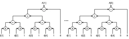
Figure 3: Generic Expressions
x
(a) Pipelined circuit for
i*c+i*c+i*c+i*c>>c
Figure 4: Pipeline circuit for repeats in generic expres-sion as given in Figure 3
3. Problem Statement
3.1. Motivational example
We will use the simple example shown in Example 1 in the rest of the paper to illustrate the RVE technique and to show how we can perform the computation in Example 1 in a pipeline fashion. d[1], d[2], d[3] and d[4] are the four inputs and A[1], A[2], ..., A[5] are the five outputs to Example 1. After applying the RVE, we get theexpanded expressionsshown in Figure 1. As all loop carried dependencies are removed, all the expanded statements in Figure 1 can be computed efficiently by computing all the outputs in parallel by using a binary tree structure for each output as shown in Figure 2. Computing like this gives a lot of parallelism, at the same time it requires a lot of area. This area can be reduced at the cost of little degradation in parallelism if all the circuits can be pipelined.
means that the sequence and type of operators in a circuit of all outputs is the same. Therefore, we can map a circuit for an output along with intermediate registers on to an FPGA as shown in Figure 4a, provided it meets the area and memory constraints. The rest of the elements can be pipelined one after the other just by feeding the corresponding variables after each cycle in the circuit. However, if the memory or area constraints are not met, then the expression for an element has to be divided further and further into some smaller repeated equivalent sub-expressions such that when a circuit is to be made for any of those sub-expressions, it satisfies the area and mem-ory constraints. This smaller sub-expression can be pipelined easily as small enough to satisfy the area and memory constraints and there are more than one such expression, for which corresponding data can be provided accordingly. For example in Figure 3, some smaller repeats are: i*c+i*c repeated 10 times and i*c repeated 20 times. The corresponding pipelined circuits are shown in Figure 4b and Figure 4c. This means that the problem of enumerating pipelining candidates for expanded expression is equivalent to finding repeated equivalent sub-expressions orrepeats in the corresponding generic expression. The chances of finding various repeats is very high in a RVE generic expression because it is generated from loop body without conditional statement which is doing some repetitive task, as shown in Figure 3.
Let E be a generic expression of length L. There can be many possible repeated sub-expressions e ∈
el1, el2, . . . , elj with corresponding number of
re-peatsn∈
nl1, nl2, . . . , nlj , whereljis the length of
the sub-expressionelj ,l1≤l2≤...≤lj andlj ≤
L 2.
The repeated sub-expressionein generic expressionE
is defined as
E= (xey)+(xey)+ (1)
wherex∈Σ∗
andy∈Σ∗
. In other words,eis any non-overlapping sub-expression inEwhich is repeated at least twice.
3.2. Problem Statement
Following are the notations used to define the prob-lem statement. Let
– E denotes the generic expression of lengthL. – AE is the estimated area required byE.
– TE is the time to transfer data for expressionE
from memory.
– TC is the time to compute the expression E on
FPGA F.
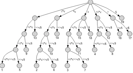
Figure 5: Suffix tree ofi*c+i*c+i*c+i*c>>c
– AF is the available area on the FPGAF.
LetAE > AF, which means expressionE as a whole
cannot be mapped on to the FPGA orTE> TC, which
means that the data transfer for expression E cannot be hidden behind computation time. Find suchk non-trivial repeated expressions eGr ∈
el1, el2, . . . , elj
of length lGr ∈ {l1, l2, . . . , lj} > 1 for 1 ≤ r ≤ k
andk≥1, which is repeated nGr time wherenGr ∈
nl1, nl2, . . . , nlj such that
nGrlGr = max
1≤i≤jnlili (2)
for which AeGr ≤ AF and TeGr ≤ TcGr. The
conditionnGrlGr ≤L is always true. where
– AeGr is the area required by the expression eGr
when mapped on to the FPGAF,
– TeGr is the time to transfer the data of expression
eGr from memory and
– TcGr is the time to compute the expression eGr
on the FPGAF.
Equation 2 mean that we choose all the k repeated expressions whose product is maximum among all expressions, when the length of each expression is multiplied with the corresponding number of times it is repeated inEand they also meet the memory and area constraints. The lengths of those expressions should be greater than 1 to make it non-trivial.
Finally we would choose the repeat e and call it optimal repeat, which satisfy Equation 2 and the following equation.
e= (
eGm |lGm = maxlGr
∀eGr
)
(3)
Equation 3 means that we will choose the expression
eGm, which has the maximum length among all eGr
4. Flexible Pipelining Design Algorithm
This section describes the flexible pipelining design algorithm. Three main steps in our algorithm are as follows:
4.1. Find possible candidates for pipelining
As mentioned in Section 3.1, finding all possible candidates for pipelining is equivalent to finding all repeats in a generic expression E. The simplest ap-proach to find all candidate expressions is to start from a pattern of length 2 and find all the repeated expressions for all the possible patterns of length 2 in the expression E of lengthL. Increase the pattern length by one and try to find the repeated expressions for all the patterns of that length until we get some pattern lengthl+ 1for which repeated pattern is not found for any possible pattern of that length. This means that the last pattern length l for which there were some repeated expression or expressions is the largest repeat. The upper bound forl is L2. If we use one of the best string matching algorithm like Knuth-Morris-Pratt [18], string matching for one pattern will take Θ(L), as there are Θ(L) possible patterns for any pattern lengthl ≤ L
2. Therefore to find repeated
pattern for one pattern length will take Θ(L2)
. Since the possible pattern lengths can be L2−1ranging from 2 to L2, it will takeΘ(L
3)
to find the optimal repeat. We will now describe a better repeat finding algo-rithm using suffix tree, well known in Bioinformatics [19]. It can find the optimal repeat inO(L2
)instead of Θ(L3
)as described earlier. A stringSis terminated by an end marker$. A suffix treeTfor a lengthLstringS$ has leaf nodes numbered1toL. The edge labels on the path from root to each leaf nodeigive a suffixS[i..L]. Every internal node except the root has at least two children. The starting character of the label of every edge coming out of a node is unique. It can be better understood by the example shown in Figure 5, which is a suffix tree for the string i*c+i*c+i*c+i*c>>c. The suffix tree for L length string is built in O(L) [20]. Once a suffix tree is built, finding a repeat is trivial, as the path from the root to any internal node represents a repeat, which can be found inO(L). There can be no more than O(L)internal nodes or repeats, as there are Lleaf nodes and every internal node has at least two children, therefore it won’t take more thanO(L2
)to find the optimal repeat. In Figure 5, all nodes without labels are internal nodes, each defining a repeat. Some of the repeats ini*c+i*c+i*c+i*c>>c as shown by Figure 5 are i*c+i*c+i*c, *c+i*c+i*c, +i*c+i*c, i*c+i*cand*c+i*c.
By making a suffix tree for the generic expression
E shown in Figure 3, it gives us all the repeats along with their start positions in E. Every repeat is a candidate for converting into a circuit for pipelining. The list of repeats can be refined by removing non-valid repeats like *c+i*c+i*c, +i*c+i*c, *c+i*c etc. To remove non-valid repeats, we fully parenthesize the generic expression E according to the priority of the operators to make it((i*c)+(i*c)+(i*c)+(i*c)>>c) and then build suffix tree from it. We filter only those repeats which are properly parenthesized and remove any substring after matching closing parenthesizes. For example, non-trivial valid repeats in parenthesized E
are (i*c),(i*c)+(i*c)and(i*c)+(i*c)+(i*c) . The non trivial non-overlapping valid repeats in parenthesized
E are (i*c)and(i*c)+(i*c).
4.2. Select the optimal repeat from among the
possible candidates.
Once the candidate repeats are shortlisted, we find the effective lengths of the repeats by removing all the parenthesizes and apply Equation 2 and Equation 3 for all of them to get the optimal repeat. In the exam-ple, the shortlisted candidates from generic expression i*c+i*c+i*c+i*c>>c are (i*c) and (i*c)+(i*c) with effective lengths 3 and 7 and frequencies 4 and 2 respectively.Applying Equation 2 givesmax(3×4,7×
2) = 7× 2, which selects (i*c)+(i*c) considering it satisfies the memory and area constraints as the only option, which becomes the optimal repeat after applying Equation 3. We call our algorithm a flexible pipelining design algorithm as it chooses the best among many candidates with different area and mem-ory requirement and can adapt when the requirements are changed.
4.3. Convert optimal repeat to a pipeline
cir-cuit.
Once the optimal repeat e is selected, it is con-verted to a deep pipelined circuit and mapped on to the FPGA. When e is evaluated, then expression
E can be computed serially as given by Equation 1 either on GPP or FPGA. In the given example,
E=i*c+i*c+i*c+i*c>>c and let the optimal repeat
e=i*c+i*c, then e is computed for two different sets of input using the pipelined circuit in Figure 4b and let the results are temporarily saved as e1
and e2
Example 2 Computing kernel in Example 1 using optimal repeati*c+i*c
for i=1 to 5
A[i]=e1
+e2
>>8 (E)
end for
Datapath for E RI RO
Memory
Stage I Stage I Stage II
Figure 6: Architecture to balance datapath with mem-ory access
inputs of the pipeline are extracted by comparing the generic expression with the expanded expression in the all the regions where eis repeated, as there is one to one correspondence between the expanded expression and generic expression.
After applying the pipelining to an expanded expres-sionE, it is divided into very few serial computations as compared to number of iterations of the loop body, which means extensive parallelism. Beside extensive parallelism, another advantage of finding the optimal repeat is the minimal memory accesses, as a lot of the expanded expression E is computed in a large pipelined circuit forewithout saving the intermediary results in the memory.
If the kernel produces some number of output vari-ables. When RVE is applied to those output variables, then it is recommended that the length of the generic expression for those output variables should be the same as in Figure 3, the length of the generic ex-pression for all the 5 outputs is the same. This is a limitation for the current pipelining algorithm. How-ever, there are many kernels from real life applications which satisfy this limitation like DCT, Finite Impulse Response (FIR) filter, Fast Fourier transform (FFT) and Matrix Multiplication.
Tr Tc
Tc
Tc
Tp
0 1 2 3 4 5
Tw
Tw
Tw
Tp
Tp
Tp
Tp
Tr
Tr
Figure 7: 2 stage pipelining, whenTp=Tc≥Tr+Tw
Table 1: Memory access time for a kernel of DCT
Description cycles
Time to read 8-bit 64 elements 8×64
64 ×3 = 24 Time to transfer 2 parameters 2×3 = 6 Time to write 9-bit 64 elements 9×64
64 ×1 = 9
Total memory access time 39
Table 3: Design time comparison of hand Optimized DCT with our automated approach
Description Design time
Hand optimized DCT > 1 man-month
Our automated DCT ≈5 sec
5. Architecture for balancing data path
and memory access operation
Usually kernels are continually run in many appli-cations. In the current FPGA board, it is not possible to read from and write to memory at the same time, therefore it is recommended to divide the kernel com-putation as a two stage pipeline as shown in Figure 6. In the first stage, all the data computed earlier and saved in register set RO is written to the on
chip memory, then data for the next iteration of the kernel is read from the memory into a register set
RI for one run of the kernel . In the second stage,
data is read fromRI and datapath operations are done
and output is saved in register set RO as shown in
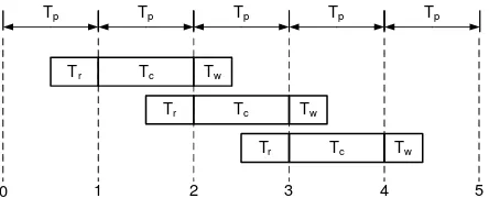
Figure 6. As both the stages read/write(Stage I) and computation(Stage II) use their own resources, we can pipeline them as shown in Figure 7 and call it memory-computation pipeline. Let the time for reading memory, doing datapath operations and writing back to memory are Tr,Tc and Tw respectively. The latency
of this pipeline is defined asTp= max(Tr+Tw, Tc).
The best is to choose the largest datapath for which
Tp=Tc≥Tr+Twprovided it also fits the area on the
FPGA. By doing this, memory access latency is totally concealed and datapath is being computed efficiently in every stage by using the optimal resources. The pipelining approach in Section 4 is different from what is discussed here as the pipelining in Section 4 refers to pipelining in datapath operations. Reading at the beginning and writing to the memory at the end of the kernel has two advantages as the total time to access the memory is minimized as all ports are used on every cycle and secondly the ordering of the accesses does not matter.
6. Experiments
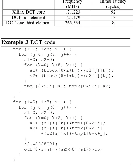
se-Table 2: Comparison of automatically optimized DCT with Xilinx hand optimized DCT
Frequency (MHz)
Initial latency (cycles)
Computation time for a block of8×8
(cycles)
Time (ns)
Slices
Xilinx DCT core 171.223 92 64 373.8 1213
DCT full element 121.479 13 64 526.8 9215
DCT one-third element 265.354 8 192 723.6 2031
Example 3DCT code for (i=0; i<8; i++) {
for (j=0; j<8; j++) { s1=0; s2=0;
for (k=0; k<8; k++) {
s1+=(block[8*i+k])*(c1[j][k]); s2+=(block[8*i+k])*(c2[j][k]); }
tmp1[8*i+j]=s1; tmp2[8*i+j]=s2; }
}
for (i=0; i<8; i++) { for (j=0; j<8; j++) {
s1=0; s2=0;
for (k=0; k<8; k++) {
s1+=(c1[i][k])*tmp1[8*k+j]; s2+=(c1[i][k])*tmp2[8*k+j]
+(c2[i][k])*tmp1[8*k+j]; }
s2+=8388591;
out[8*i+j]=((s2>>8)+s1)>>16; }
}
lected platform and kernel and finally we will show and discuss our results.
We have implemented the RVE transformation, find-ing repeats in an expression and givfind-ing all the short-listed candidates for pipelining short-listed in ascending order with their lengths to estimate the area and time to transfer the data. The user can choose the first sub-expression that fits memory and area requirements in that order. The variables that need to be transferred after every cycle in the start of the pipeline shown in Figure 4 are generated automatically for the chosen re-peated sub-expression. Finally, a synthesizable VHDL code is also generated automatically.
We use a Molen [15] prototype implemented on the Xilinx Virtex II pro platform XC2VP30 FPGA, which contains 13696 slices. The automatically generated code was simulated and synthesized on ModelSIM and Xilinx XST of ISE 8.2.022 respectively.
To evaluate and demonstrate the pipelining algo-rithm for RVE, we have used an integer implemen-tation of DCT as given in Example 3, which satisfies all the constraints of the technique given in Sections 2.1 and 4. The results of the automatically optimized and different pipeline sizes for the DCT are compared with the hand optimized and pipelined DCT core
(https://secure.xilinx.com/webreg/clickthrough.do?cid=55758)
pro-vided by Xilinx on the same platform. All the imple-mentations take 8-bit input block elements and output DCT of 9-bit. The port size to access on chip memory is 64 bits, which means at most 64 bits can be read or write simultaneously. It takes 3 cycles to read from on chip memory and store it in register set RI, whereas
it takes 1 cycle to write fromRO to on chip memory.
The total memory access time to transfer the data for a block of DCT is 39 cycles as given in Table 1.
A kernel of DCT outputs 64 elements whose generic expressions are the same. The repeat finding algorithm gives the optimal repeat in generic equation to be equal to expanded expression of one of these elements, we refer to it as full element in the experiment. This is the largest repeat which satisfy the area and memory requirements, therefore it is the optimal repeat. How-ever, if there is less area available on FPGA, The next largest repeat is equal to one third of the expanded expression of the element, we refer to it as one-third element.
Table 2 shows the results for different implementa-tion of DCT after synthesis. The Xilinx DCT core is hand optimized by knowing the properties of 2D DCT. In it, 1D DCT is only implemented with buffering and taking the transpose of the 8×8 block. Initially 1D DCT is computed from the inputs, then the output is transposed and fed back to the same 1D DCT circuit to produce 2D DCT. The generated code is very small and well pipelined, therefore it has very few slices and high frequency. However the initial latency is high due to transposition and computing again the 1DCT. Once the initial latency is spent, the circuit produces an entire DCT block every 64 cycles.
the pipeline. The code for DCT one-third is relatively small but still larger than Xilinx DCT core. It produces better frequency than Xilinx core at the cost of 3 times more cycles and low initial latency of 8 cycles to compute one DCT block. The time to compute DCT using one third element is increased by 37% with a 78% decrease in area as compared to computing with full element.
The results show that our pipelining design algo-rithm for RVE which applies on some limited type of problems gives a comparable performance at the cost of extra hardware than the hand optimized code. Although it is not better than hand optimized in perfor-mance, the main benefits of our approach is automated design, optimization, and HW generation of kernels starting from a program code. The design time for the two approaches is shown in Table 3, which shows that our approach due to automation takes negligible time as compared to hand optimized DCT and produces comparably fast circuit.
7. Conclusion
In this paper, we have presented a pipelining al-gorithm for RVE, which automatically generates an extensively parallel and pipelined VHDL code for a certain class of problems, which can compare in performance with hand optimized codes. Although the algorithm produce better performance for large area FPGA, still it can be used to get good performance for reasonably small FPGA. Our algorithm is a good choice for kernels which satisfy the given constraints for which hand optimized codes are not available, area is not major concern and high performance is the requirement in short design time. As a future work, we will apply our algorithm on more kernels for real life application and remove the equal size constraint of generic expressions for different outputs.
Acknowledgments
Delft Workbench is sponsored by the hArtes (IST-035143), the MORPHEUS (IST-027342) and RCOSY (DES-6392) projects. Also, we would like to thank Mudassir Shabbir.
References
[1] D. F. Baconet al., “Compiler transformations for high-performance computing,”ACM Comput. Surv., vol. 26, pp. 345–420, 1994.
[2] Z. Nawazet al., “Recursive variable expansion: A loop transformation for reconfigurable systems,” inICFPT 2007, 2007.
[3] V. H. Allanet al., “Software pipelining,”ACM Comput. Surv., vol. 27, pp. 367–432, 1995.
[4] T. J. Callahanet al., “Adapting software pipelining for reconfigurable computing,” inCASES ’00, 2000. [5] M. B. Gokhale et al., “Co-synthesis to a hybrid
risc/fpga architecture,” J. VLSI Signal Process. Syst., vol. 24, pp. 165–180, 2000.
[6] R. Schreiber et al., “High-level synthesis of nonpro-grammable hardware accelerators,” inASAP ’00, 2000. [7] G. Snider, “Performance-constrained pipelining of soft-ware loops onto reconfigurable hardsoft-ware,” in FPGA ’02, 2002.
[8] C. E. Leiserson et al., “Retiming synchronous cir-cuitry,”Algorithmica, vol. 6, pp. 5–35, 1991.
[9] M. Weinhardt et al., “Pipeline vectorization,” IEEE Transactions on CAD, vol. 20(2), pp. 234–248, 2001. [10] D. Petkovet al., “Efficient pipelining of nested loops:
Unroll-and-squash,” inIPDPS 02, 2002.
[11] H. E. Ziegler et al., “Compiler-generated communica-tion for piplined fpga applicacommunica-tions,” inDAC2003, 2003. [12] H. Styles et al., “Pipelining design with loop carried
dependencies,” inICFPT2004, 2004.
[13] A. H. Veen, “Dataflow machine architecture,” ACM Computing Surveys, vol. 18(4), 1986.
[14] R. Rodrigues et al., “A data-driven approach for pipelining sequences of data-dependent loops,” in
FCCM ’07, 2007.
[15] S. Vassiliadiset al., “The molen polymorphic proces-sor,”IEEE Transactions on Computers, pp. 1363– 1375, 2004.
[16] D. Kuck et al., “On the number of operations simul-taneously executable in fortran-like programs and their resulting speedup,”Transactions on Computers, vol. C-21, pp. 1293– 1310, 1972.
[17] Z. Nawazet al., “Acceleration of smith-waterman using recursive variable expansion,” inDSD’08, 2008. [18] D. E. Knuthet al., “Fast pattern matching in strings,”
SIAM Journal on Computing, vol. 6, pp. 323–350, 1977.
[19] D. Gusfield, Algorithms on Strings, Trees and Se-quences: Computer Science and Computational Biol-ogy. Cambridge University Press, 1997.
[20] E. Ukkonen, “On-line construction of suffix trees,”