Chapter 29
Magnetic Fields
C H A P T E R O U T L I N E
29.1
Magnetic Fields and Forces
29.2
Magnetic Force Acting on a
Current-Carrying Conductor
29.3
Torque on a Current Loop in a
Uniform Magnetic Field
29.4
Motion of a Charged Particle
in a Uniform Magnetic Field
29.5
Applications Involving
Charged Particles Moving in a
Magnetic Field
29.6
The Hall Effect
894
895
M
any historians of science believe that the compass, which uses a magnetic needle,was used in China as early as the 13th century B.C., its invention being of Arabic or Indian origin. The early Greeks knew about magnetism as early as 800 B.C. They discov-ered that the stone magnetite (Fe3O4) attracts pieces of iron. Legend ascribes the name magnetite to the shepherd Magnes, the nails of whose shoes and the tip of whose staff stuck fast to chunks of magnetite while he pastured his flocks.
In 1269 a Frenchman named Pierre de Maricourt found that the directions of a needle near a spherical natural magnet formed lines that encircled the sphere and passed through two points diametrically opposite each other, which he called the poles of the magnet. Subsequent experiments showed that every magnet, regardless of its shape, has two poles, called north (N) and south (S) poles, that exert forces on other magnetic poles similar to the way that electric charges exert forces on one another. That is, like poles (N–N or S–S) repel each other, and opposite poles (N–S) attract each other.
The poles received their names because of the way a magnet, such as that in a compass, behaves in the presence of the Earth’s magnetic field. If a bar magnet is sus-pended from its midpoint and can swing freely in a horizontal plane, it will rotate until its north pole points to the Earth’s geographic North Pole and its south pole points to the Earth’s geographic South Pole.1
In 1600 William Gilbert (1540–1603) extended de Maricourt’s experiments to a variety of materials. Using the fact that a compass needle orients in preferred directions, he suggested that the Earth itself is a large permanent magnet. In 1750 experimenters used a torsion balance to show that magnetic poles exert attractive or repulsive forces on each other and that these forces vary as the inverse square of the distance between in-teracting poles. Although the force between two magnetic poles is otherwise similar to the force between two electric charges, electric charges can be isolated (witness the electron and proton) whereas a single magnetic pole has never been isolated.That is, magnetic poles are always found in pairs. All attempts thus far to detect an isolated magnetic pole have been unsuccessful. No matter how many times a permanent magnet is cut in two, each piece always has a north and a south pole.2
The relationship between magnetism and electricity was discovered in 1819 when, during a lecture demonstration, the Danish scientist Hans Christian Oersted found that an electric current in a wire deflected a nearby compass needle.3In the 1820s,
1 Note that the Earth’s geographic North Pole is magnetically a south pole, whereas its
geo-graphic South Pole is magnetically a north pole. Because oppositemagnetic poles attract each
other, the pole on a magnet that is attracted to the Earth’s geographic North Pole is the magnet’s northpole and the pole attracted to the Earth’s geographic South Pole is the magnet’s south pole.
2 There is some theoretical basis for speculating that magnetic monopoles—isolated north or
south poles—may exist in nature, and attempts to detect them are an active experimental field of investigation.
3 The same discovery was reported in 1802 by an Italian jurist, Gian Dominico Romognosi, but
was overlooked, probably because it was published in an obscure journal.
Hans Christian
Oersted
Danish Physicist and Chemist (1777–1851)
further connections between electricity and magnetism were demonstrated indepen-dently by Faraday and Joseph Henry (1797–1878). They showed that an electric current can be produced in a circuit either by moving a magnet near the circuit or by changing the current in a nearby circuit. These observations demonstrate that a changing magnetic field creates an electric field. Years later, theoretical work by Maxwell showed that the reverse is also true: a changing electric field creates a mag-netic field.
This chapter examines the forces that act on moving charges and on current-carrying wires in the presence of a magnetic field. The source of the magnetic field is described in Chapter 30.
29.1
Magnetic Fields and Forces
In our study of electricity, we described the interactions between charged objects in terms of electric fields. Recall that an electric field surrounds any electric charge. In addition to containing an electric field, the region of space surrounding any moving electric charge also contains a magnetic field. A magnetic field also surrounds a mag-netic substance making up a permanent magnet.
Historically, the symbol B has been used to represent a magnetic field, and this is the notation we use in this text. The direction of the magnetic field Bat any loca-tion is the direcloca-tion in which a compass needle points at that localoca-tion. As with the electric field, we can represent the magnetic field by means of drawings with mag-netic field lines.
Figure 29.1 shows how the magnetic field lines of a bar magnet can be traced with the aid of a compass. Note that the magnetic field lines outside the magnet point away from north poles and toward south poles. One can display magnetic field patterns of a bar magnet using small iron filings, as shown in Figure 29.2.
We can define a magnetic field Bat some point in space in terms of the magnetic force FBthat the field exerts on a charged particle moving with a velocity v, which we
call the test object. For the time being, let us assume that no electric or gravitational fields are present at the location of the test object. Experiments on various charged particles moving in a magnetic field give the following results:
• The magnitude FBof the magnetic force exerted on the particle is proportional to
the charge qand to the speed vof the particle.
• The magnitude and direction of FBdepend on the velocity of the particle and on
the magnitude and direction of the magnetic field B.
• When a charged particle moves parallel to the magnetic field vector, the magnetic force acting on the particle is zero.
Properties of the magnetic force on a charge moving in a mag-netic field B
N S
Active Figure 29.1 Compass needles can be used to trace the magnetic field lines in the region outside a bar magnet.
S E C T I O N 2 9 . 1 • Magnetic Fields and Forces 897
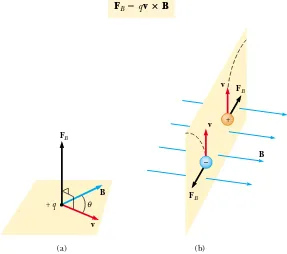
• When the particle’s velocity vector makes any angle !!0 with the magnetic field,
the magnetic force acts in a direction perpendicular to both vand B; that is, FBis
perpendicular to the plane formed by vand B(Fig. 29.3a).
• The magnetic force exerted on a positive charge is in the direction opposite the direction of the magnetic force exerted on a negative charge moving in the same direction (Fig. 29.3b).
• The magnitude of the magnetic force exerted on the moving particle is propor-tional to sin !, where ! is the angle the particle’s velocity vector makes with the direction of B.
We can summarize these observations by writing the magnetic force in the form
(29.1) FB"qv!B
(a) (b) (c)
Figure 29.2 (a) Magnetic field pattern surrounding a bar magnet as displayed with iron filings. (b) Magnetic field pattern between opposite poles (N–S) of two bar magnets. (c) Magnetic field pattern between like poles (N–N) of two bar magnets.
(a) FB
B + q
v θ
(b) FB
B –
v v F
B
+
Figure 29.3 The direction of the magnetic force FBacting on a charged particle moving with a velocity vin the presence of a magnetic field B. (a) The magnetic force is perpendicular to both vand B. (b) Oppositely directed magnetic forces FBare exerted on two oppositely charged particles moving at the same velocity in a magnetic field. The dashed lines show the paths of the particles, which we will investigate in Section 29.4.
Henry Leap and Jim Lehman
which by definition of the cross product (see Section 11.1) is perpendicular to both v and B. We can regard this equation as an operational definition of the magnetic field at some point in space. That is, the magnetic field is defined in terms of the force acting on a moving charged particle.
Figure 29.4 reviews two right-hand rules for determining the direction of the cross product v!B and determining the direction of FB. The rule in Figure 29.4a depends on our right-hand rule for the cross product in Figure 11.2. Point the four fingers of your right hand along the direction of vwith the palm facing B and curl them toward B. The extended thumb, which is at a right angle to the fingers, points in the direction of v!B. Because FB"qv!B, FBis in the direction of your thumb if q is positive and opposite the direction of your thumb if q is negative. (If you need more help understanding the cross product, you should review pages 337 to 339, in-cluding Fig. 11.2.)
An alternative rule is shown in Figure 29.4b. Here the thumb points in the direc-tion of vand the extended fingers in the direction of B. Now, the force FB on a posi-tive charge extends outward from your palm. The advantage of this rule is that the force on the charge is in the direction that you would push on something with your hand—outward from your palm. The force on a negative charge is in the opposite direction. Feel free to use either of these two right-hand rules.
The magnitude of the magnetic force on a charged particle is
(29.2) where !is the smaller angle between vand B. From this expression, we see that FBis zero when vis parallel or antiparallel to B (! "0 or 180°) and maximum when v is perpendicular to B(! "90°).
There are several important differences between electric and magnetic forces:
• The electric force acts along the direction of the electric field, whereas the mag-netic force acts perpendicular to the magmag-netic field.
• The electric force acts on a charged particle regardless of whether the particle is moving, whereas the magnetic force acts on a charged particle only when the parti-cle is in motion.
FB" !q!vB sin ! B FB
B v
(a)
v
(b) FB
Figure 29.4 Two right-hand rules for determining the direction of the magnetic force FB"qv!Bacting on a particle with charge qmoving with a velocity vin a magnetic field B. (a) In this rule, the fingers point in the direction of v, with Bcoming out of your palm, so that you can curl your fingers in the direction of B. The direction of v!B, and the force on a positive charge, is the direction in which the thumb points. (b) In this rule, the vector vis in the direction of your thumb and Bin the direction of your fingers. The force FBon a positive charge is in the direction of your palm, as if you are pushing the particle with your hand.
S E C T I O N 2 9 . 1 • Magnetic Fields and Forces 899
• The electric force does work in displacing a charged particle, whereas the magnetic force associated with a steady magnetic field does no work when a particle is dis-placed because the force is perpendicular to the displacement.
From the last statement and on the basis of the work–kinetic energy theorem, we conclude that the kinetic energy of a charged particle moving through a magnetic field cannot be altered by the magnetic field alone. In other words, when a charged particle moves with a velocity v through a magnetic field, the field can alter the direction of the velocity vector but cannot change the speed or kinetic energy of the particle.
From Equation 29.2, we see that the SI unit of magnetic field is the newton per coulomb-meter per second, which is called the tesla(T):
Because a coulomb per second is defined to be an ampere, we see that
A non-SI magnetic-field unit in common use, called the gauss(G), is related to the tesla through the conversion 1 T"104G. Table 29.1 shows some typical values of
mag-netic fields.
1 T"1 N A#m 1 T"1 N
C#m/s
Source of Field Field Magnitude (T)
Strong superconducting laboratory magnet 30 Strong conventional laboratory magnet 2
Medical MRI unit 1.5
Bar magnet 10$2
Surface of the Sun 10$2
Surface of the Earth 0.5%10$4
Inside human brain (due to nerve impulses) 10$13
Some Approximate Magnetic Field Magnitudes
Table 29.1
Quick Quiz 29.1
The north-pole end of a bar magnet is held near a posi-tively charged piece of plastic. Is the plastic (a) attracted, (b) repelled, or (c) unaf-fected by the magnet?Quick Quiz 29.2
A charged particle moves with velocity vin a magneticfield B. The magnetic force on the particle is a maximum when vis (a) parallel to B, (b) perpendicular to B, (c) zero.
Quick Quiz 29.3
An electron moves in the plane of this paper toward the top of the page. A magnetic field is also in the plane of the page and directed toward the right. The direction of the magnetic force on the electron is (a) toward the top of the page, (b) toward the bottom of the page, (c) toward the left edge of the page, (d) toward the right edge of the page, (e) upward out of the page, (f) downward into the page.29.2
Magnetic Force Acting on a Current-Carrying
Conductor
If a magnetic force is exerted on a single charged particle when the particle moves through a magnetic field, it should not surprise you that a current-carrying wire also experiences a force when placed in a magnetic field. This follows from the fact that the current is a collection of many charged particles in motion; hence, the resultant force exerted by the field on the wire is the vector sum of the individual forces exerted on all the charged particles making up the current. The force exerted on the particles is transmitted to the wire when the particles collide with the atoms making up the wire. Before we continue our discussion, some explanation of the notation used in this book is in order. To indicate the direction of B in illustrations, we sometimes present perspective views, such as those in Figure 29.5. If B lies in the plane of the page or is present in a perspective drawing, we use blue vectors or blue field lines with arrowheads. In non-perspective illustrations, we depict a magnetic field
Example 29.1 An Electron Moving in a Magnetic Field
An electron in a television picture tube moves toward the front of the tube with a speed of 8.0%106m/s along the x axis (Fig. 29.5). Surrounding the neck of the tube are coils of wire that create a magnetic field of magnitude 0.025 T, directed at an angle of 60°to the xaxis and lying in the xy plane.
(A) Calculate the magnetic force on the electron using Equation 29.2.
Solution Using Equation 29.2, we find the magnitude of the magnetic force:
2.8%10$14 N
"
"(1.6%10$19 C)(8.0%106 m/s)(0.025 T)(sin 60&)
FB" !q!vBsin !
Because v!Bis in the positive zdirection (from the right-hand rule) and the charge is negative, FBis in the negative z direction.
(B) Find a vector expression for the magnetic force on the electron using Equation 29.1.
Solution We begin by writing a vector expression for the velocity of the electron:
and one for the magnetic field:
The force on the electron, using Equation 29.1, is
where we have used Equations 11.7a and 11.7b to eva-luate and . Carrying out the multiplication, we
find,
This expression agrees with the result in part (A). The mag-nitude is the same as we found there, and the force vector is in the negative zdirection.
($2.8%10$14 N)ˆk FB"
iˆ!jˆ i
ˆ!ˆi
"($1.6%10$19 C)(8.0%106 m/s)(0.022 T)ˆk '($e)(8.0%106 m/s)(0.022 T)(ˆi!ˆj) "($e)(8.0%106 m/s)(0.013 T)(ˆi!ˆi)
'($e)[(8.0%106ˆi) m/s]%[(0.022ˆj)T] "($e)[(8.0%106ˆi) m/s]%[(0.013ˆi)T]
"($e)[(8.0%106ˆi) m/s]%[(0.013ˆi'0.022ˆj)T] FB"q v%B
"(0.013ˆi'0.022ˆj)T
B"(0.025 cos 60&ˆi '0.025 sin 60&ˆj)T v"(8.0%106ˆi) m/s
z
B
v
y
x
FB 60°
–e
S E C T I O N 2 9 . 2 • Magnetic Force Acting on a Current-Carrying Conductor 901
perpendicular to and directed out of the page with a series of blue dots, which represent the tips of arrows coming toward you (see Fig. 29.6a). In this case, we label the field Bout. If Bis directed perpendicularly into the page, we use blue crosses, which represent the feathered tails of arrows fired away from you, as in Figure 29.6b. In this case, we label the field Bin, where the subscript “in” indicates “into the page.” The same notation with crosses and dots is also used for other quantities that might be per-pendicular to the page, such as forces and current directions.
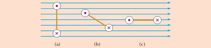
One can demonstrate the magnetic force acting on a current-carrying conductor by hanging a wire between the poles of a magnet, as shown in Figure 29.7a. For ease in visualization, part of the horseshoe magnet in part (a) is removed to show the end face of the south pole in parts (b), (c), and (d) of Figure 29.7. The magnetic field is directed into the page and covers the region within the shaded squares. When the current in the wire is zero, the wire remains vertical, as shown in Figure 29.7b. However, when the wire carries a current directed upward, as shown in Figure 29.7c, the wire deflects to the left. If we reverse the current, as shown in Figure 29.7d, the wire deflects to the right.
Let us quantify this discussion by considering a straight segment of wire of length L
and cross-sectional area A, carrying a current Iin a uniform magnetic field B, as shown in Figure 29.8. The magnetic force exerted on a charge qmoving with a drift velocity vdis qvd!B. To find the total force acting on the wire, we multiply the force qvd!B exerted on one charge by the number of charges in the segment. Because the volume of the segment is AL, the number of charges in the segment is nAL, where nis the number of charges per unit volume. Hence, the total magnetic force on the wire of length Lis
We can write this expression in a more convenient form by noting that, from Equation 27.4, the current in the wire is I"nqvdA. Therefore,
(29.3)
where Lis a vector that points in the direction of the current Iand has a magnitude equal to the length L of the segment. Note that this expression applies only to a straight segment of wire in a uniform magnetic field.
FB"I L!B
Figure 29.6 (a) Magnetic field lines coming out of the paper are indicated by dots, representing the tips of arrows coming outward. (b) Magnetic field lines going into the paper are indicated by crosses, representing the feathers of arrows
Figure 29.7 (a) A wire suspended vertically between the poles of a magnet. (b) The setup shown in part (a) as seen looking at the south pole of the magnet, so that the magnetic field (blue crosses) is directed into the page. When there is no current in the wire, it remains vertical. (c) When the current is upward, the wire deflects to the left. (d) When the current is downward, the wire deflects to the right.
q
Figure 29.8 A segment of a current-carrying wire in a magnetic field B. The magnetic force exerted on each charge making up the current is qvd!Band the net force on the segment of length Lis IL!B.
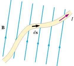
Now consider an arbitrarily shaped wire segment of uniform cross section in a magnetic field, as shown in Figure 29.9. It follows from Equation 29.3 that the magnetic force exerted on a small segment of vector length dsin the presence of a field Bis
(29.4) where dFBis directed out of the page for the directions of Band dsin Figure 29.9. We can consider Equation 29.4 as an alternative definition of B. That is, we can define the magnetic field Bin terms of a measurable force exerted on a current element, where the force is a maximum when Bis perpendicular to the element and zero when B is parallel to the element.
To calculate the total force FBacting on the wire shown in Figure 29.9, we integrate Equation 29.4 over the length of the wire:
(29.5)
where aand b represent the end points of the wire. When this integration is carried out, the magnitude of the magnetic field and the direction the field makes with the vector dsmay differ at different points.
We now treat two interesting special cases involving Equation 29.5. In both cases, the magnetic field is assumed to be uniform in magnitude and direction.
Case 1. A curved wire carries a current Iand is located in a uniform magnetic field B, as shown in Figure 29.10a. Because the field is uniform, we can take B outside the integral in Equation 29.5, and we obtain
(29.6)
But the quantity dsrepresents the vector sum of all the length elements from ato b. From the law of vector addition, the sum equals the vector L(, directed from ato b. Therefore, Equation 29.6 reduces to
(29.7)
From this we conclude that the magnetic force on a curved current-carrying wire in a uniform magnetic field is equal to that on a straight wire connecting the end points and carrying the same current.
FB"I L(!B "b
a
FB"I
#
"
b a ds$
!B FB"I
"
b a d
s!B
dFB"Ids!B B
ds
I
Figure 29.9 A wire segment of arbitrary shape carrying a current I in a magnetic field Bexperiences a magnetic force. The magnetic force on any segment dsis I ds!B and is directed out of the page. You should use the right-hand rule to confirm this force direction.
(b) ds
B I
I b
a ds
L′ B
(a)
S E C T I O N 2 9 . 2 • Magnetic Force Acting on a Current-Carrying Conductor 903
Case 2. An arbitrarily shaped closed loop carrying a current Iis placed in a uniform magnetic field, as shown in Figure 29.10b. We can again express the magnetic force acting on the loop in the form of Equation 29.6, but this time we must take the vector sum of the length elements dsover the entire loop:
Because the set of length elements forms a closed polygon, the vector sum must be zero. This follows from the procedure for adding vectors by the graphical method. Because %ds"0, we conclude that FB"0; that is, the net magnetic force acting on any closed current loop in a uniform magnetic field is zero.
FB"I
#
&
ds$
!BQuick Quiz 29.4
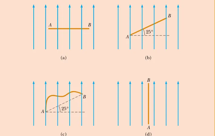
The four wires shown in Figure 29.11 all carry the same current from point Ato point Bthrough the same magnetic field. In all four parts of the figure, the points Aand Bare 10 cm apart. Rank the wires according to the magni-tude of the magnetic force exerted on them, from greatest to least.Quick Quiz 29.5
A wire carries current in the plane of this paper toward the top of the page. The wire experiences a magnetic force toward the right edge of the page. The direction of the magnetic field causing this force is (a) in the plane of the page and toward the left edge, (b) in the plane of the page and toward the bottom edge, (c) upward out of the page, (d) downward into the page.A B
A
B
25°
A B
25° B
A
(a) (b)
(c) (d)
Figure 29.11 (Quick Quiz 29.4) Which wire experiences the greatest magnetic force?
Example 29.2 Force on a Semicircular Conductor
A wire bent into a semicircle of radius Rforms a closed circuit and carries a current I. The wire lies in the xy plane, and a uniform magnetic field is directed along the positive y axis, as shown in Figure 29.12. Find the magnitude and direction of the magnetic force acting
on the straight portion of the wire and on the curved portion.
29.3
Torque on a Current Loop in a Uniform
Magnetic Field
In the preceding section, we showed how a magnetic force is exerted on a current-carrying conductor placed in a magnetic field. With this as a starting point, we now show that a torque is exerted on a current loop placed in a magnetic field. The results of this analysis will be of great value when we discuss motors in Chapter 31.
Consider a rectangular loop carrying a current Iin the presence of a uniform mag-netic field directed parallel to the plane of the loop, as shown in Figure 29.13a. No
shown in Figure 29.13a, and that of F4, the magnetic force exerted on wire $, is into the
page in the same view. If we view the loop from side "and sight along sides #and $, we see the view shown in Figure 29.13b, and the two magnetic forces F2and F4are
di-rected as shown. Note that the two forces point in opposite directions but are not di-rected along the same line of action. If the loop is pivoted so that it can rotate about point O, these two forces produce about Oa torque that rotates the loop clockwise. The magnitude of this torque )maxis
where the moment arm about Ois b/2 for each force. Because the area enclosed by the loop is A"ab, we can express the maximum torque as
(29.8)
This maximum-torque result is valid only when the magnetic field is parallel to the plane of the loop. The sense of the rotation is clockwise when viewed from side ", as indicated in Figure 29.13b. If the current direction were reversed, the force directions would also reverse, and the rotational tendency would be counterclockwise.
)max"IAB the wire is oriented perpendicular to B. The direction of F1
is out of the page based on the right-hand rule for the cross product L!B.
To find the magnetic force F2acting on the curved part, we use the results of Case 1. The magnetic force on the curved portion is the same as that on a straight wire of length 2Rcarrying current Ito the left. Thus, F2"ILB" 2IR B. The direction of F2 is into the page based on the right-hand rule for the cross product L!B.
Because the wire lies in the xyplane, the two forces on the loop can be expressed as
The net magnetic force on the loop is
Note that this is consistent with Case 2, because the wire forms a closed loop in a uniform magnetic field.
'
F"F1'F2"2IRBˆk$2IRBkˆ"0Figure 29.12 (Example 29.2) The net magnetic force acting on a closed current loop in a uniform magnetic field is zero. In the setup shown here, the magnetic force on the straight portion of the loop is 2IRBand directed out of the page, and the magnetic force on the curved portion is 2IRBdirected into the page. of a rectangular current loop in a uniform magnetic field. No mag-netic forces are acting on sides !
and "because these sides are
paral-lel to B. Forces are acting on sides
#and $, however. (b) Edge view of
the loop sighting down sides #and $shows that the magnetic forces F2
and F4exerted on these sides create a torque that tends to twist the loop clockwise. The purple dot in the left circle represents current in wire #
S E C T I O N 2 9 . 3 • Torque on a Current Loop in a Uniform Magnetic Field 905
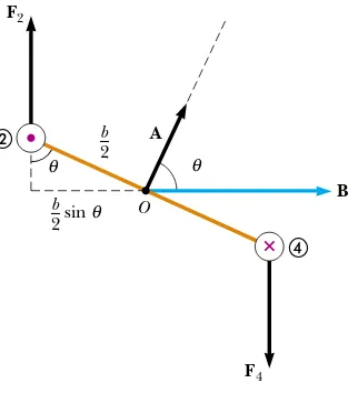
Now suppose that the uniform magnetic field makes an angle ! *90°with a line perpendicular to the plane of the loop, as in Figure 29.14. For convenience, we assume that Bis perpendicular to sides #and $. In this case, the magnetic forces F1and F3 exerted on sides !and "cancel each other and produce no torque because they pass through a common origin. However, the magnetic forces F2and F4acting on sides # and $ produce a torque about any point.Referring to the end view shown in Figure 29.14, we note that the moment arm of F2about the point Ois equal to (b/2) sin !. Likewise, the moment arm of F4about Ois also (b/2) sin !. Because F2"F4"IaB, the
magnitude of the net torque about Ois
where A"ab is the area of the loop. This result shows that the torque has its maximum value IABwhen the field is perpendicular to the normal to the plane of the loop (! "90°), as we saw when discussing Figure 29.13, and is zero when the field is parallel to the normal to the plane of the loop (! "0).
A convenient expression for the torque exerted on a loop placed in a uniform magnetic field Bis
(29.9) where A, the vector shown in Figure 29.14, is perpendicular to the plane of the loop and has a magnitude equal to the area of the loop. We determine the direction of Ausing the right-hand rule described in Figure 29.15. When you curl the fingers of your right hand in the direction of the current in the loop, your thumb points in the direction of A. As we see in Figure 29.14, the loop tends to rotate in the direction of decreasing values of ! (that is, such that the area vector Arotates toward the direction of the magnetic field).
The product IAis defined to be the magnetic dipole moment" (often simply called the “magnetic moment”) of the loop:
(29.10) The SI unit of magnetic dipole moment is ampere-meter2(A#m2). Using this definition,
we can express the torque exerted on a current-carrying loop in a magnetic field Bas
(29.11) Note that this result is analogous to Equation 26.18, #"p!E, for the torque exerted on an electric dipole in the presence of an electric field E, where p is the electric dipole moment.
# $ " !B ""IA #"IA!B "IAB sin !
"IaB
#
b2 sin !
$
'IaB#
b
2 sin !
$
"IabB sin ! ) "F2b
2 sin ! 'F4
b
2 sin ! F2
F4
O B
A
b 2 – sin θ
b 2 –
θ θ
θ
#
$
×Active Figure 29.14 An end view of the loop in Figure 29.13b rotated through an angle with respect to the magnetic field. If Bis at an angle ! with respect to vector A, which is perpendicular to the plane of the loop, the torque is IABsin !where the magnitude of Ais A, the area of the loop.
At the Active Figures link athttp://www.pse6.com, you can choose the current in the loop, the magnetic field, and the initial orientation of the loop and observe the subsequent motion.
Torque on a current loop in a magnetic field
Magnetic dipole moment of a current loop
Torque on a magnetic moment in a magnetic field
A
I µ
Although we obtained the torque for a particular orientation of Bwith respect to the loop, the equation #"" !B is valid for any orientation. Furthermore, although we derived the torque expression for a rectangular loop, the result is valid for a loop of any shape.
If a coil consists of Nturns of wire, each carrying the same current and enclosing the same area, the total magnetic dipole moment of the coil is Ntimes the magnetic dipole moment for one turn. The torque on an N-turn coil is Ntimes that on a one-turn coil. Thus, we write #"N"loop!B""coil!B.
In Section 26.6, we found that the potential energy of a system of an electric dipole in an electric field is given by U" $p!E. This energy depends on the orientation of the dipole in the electric field. Likewise, the potential energy of a system of a magnetic dipole in a magnetic field depends on the orientation of the dipole in the magnetic field and is given by
(29.12)
From this expression, we see that the system has its lowest energy Umin" $+Bwhen "
points in the same direction as B. The system has its highest energy Umax" '+Bwhen "points in the direction opposite B.
U" $" %B
Example 29.3 The Magnetic Dipole Moment of a Coil
A rectangular coil of dimensions 5.40 cm%8.50 cm consists of 25 turns of wire and carries a current of 15.0 mA. A 0.350-T magnetic field is applied parallel to the plane of the loop. (A) Calculate the magnitude of its magnetic dipole moment.
Solution Because the coil has 25 turns, we modify Equation 29.10 to obtain
1.72%10$3 A#m2
"
+coil"NIA"(25)(15.0%10$3 A)(0.054 0 m)(0.085 0 m)
(B) What is the magnitude of the torque acting on the loop?
Solution Because B is perpendicular to "coil, Equation 29.11 gives
6.02%10$4 N#m
"
) " +coilB"(1.72%10$3 A#m2)(0.350 T )
Potential energy of a system of a magnetic moment in a magnetic field
Quick Quiz 29.6
Rank the magnitudes of the torques acting on the rectan-gular loops shown edge-on in Figure 29.16, from highest to lowest. All loops are identi-cal and carry the same current.Quick Quiz 29.7
Rank the magnitudes of the net forces acting on the rec-tangular loops shown in Figure 29.16, from highest to lowest. All loops are identical and carry the same current.(a) (b) (c)
× ×
×
S E C T I O N 2 9 . 4 • Motion of a Charged Particle in a Uniform Magnetic Field 907
Example 29.4 Satellite Attitude Control
Many satellites use coils called torquers to adjust their orien-tation. These devices interact with the Earth’s magnetic field to create a torque on the spacecraft in the x, y, or z direc-tion. The major advantage of this type of attitude-control system is that it uses solar-generated electricity and so does not consume any thruster fuel.
If a typical device has a magnetic dipole moment of 250 A#m2, what is the maximum torque applied to a satellite when its torquer is turned on at an altitude where the mag-nitude of the Earth’s magnetic field is 3.0%10$5T?
Solution We once again apply Equation 29.11, recognizing that the maximum torque is obtained when the magnetic dipole moment of the torquer is perpendicular to the Earth’s magnetic field:
7.5%10$3 N#m
"
)max"+B"(250 A#m2)(3.0%10$5 T)
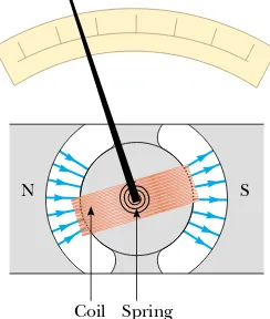
Example 29.5 The D’Arsonval Galvanometer
An end view of a D’Arsonval galvanometer (see Section 28.5) is shown in Figure 29.17. When the turns of wire mak-ing up the coil carry a current, the magnetic field created by the magnet exerts on the coil a torque that turns it (along with its attached pointer) against the spring. Show that the angle of deflection of the pointer is directly proportional to the current in the coil.
Solution We can use Equation 29.11 to find the torque )m that the magnetic field exerts on the coil. If we assume that the magnetic field through the coil is perpendicular to the normal to the plane of the coil, Equation 29.11 becomes
(This is a reasonable assumption because the circular cross section of the magnet ensures radial magnetic field lines.) This magnetic torque is opposed by the torque due to the spring, which is given by the rotational version of Hooke’s law, )s" $,-, where ,is the torsional spring constant and -is the angle through which the spring turns. Because the coil does not have an angular acceleration when the pointer is at rest, the sum of these torques must be zero:
Equation 29.10 allows us to relate the magnetic moment of the Nturns of wire to the current through them:
+ "NIA
(1)
)m')s"+B$,- "0 )m"+B
We can substitute this expression for + in Equation (1) to obtain
Thus, the angle of deflection of the pointer is directly pro-portional to the current in the loop. The factor NAB/,tells us that deflection also depends on the design of the meter.
NAB
, I
- " (NIA)B$,- "0
S
Coil N
Spring
Figure 29.17 (Example 29.5) Structure of a moving-coil galvanometer.
29.4
Motion of a Charged Particle in a Uniform
Magnetic Field
the particle is a circle! Figure 29.18 shows the particle moving in a circle in a plane perpendicular to the magnetic field.
The particle moves in a circle because the magnetic force FBis perpendicular to v and B and has a constant magnitude qvB. As Figure 29.18 illustrates, the rotation is counterclockwise for a positive charge. If q were negative, the rotation would be clockwise. We can use Equation 6.1 to equate this magnetic force to the product of the particle mass and the centripetal acceleration:
(29.13)
That is, the radius of the path is proportional to the linear momentum mvof the parti-cle and inversely proportional to the magnitude of the charge on the partiparti-cle and to the magnitude of the magnetic field. The angular speed of the particle (from Eq. 10.10) is
(29.14)
The period of the motion (the time interval the particle requires to complete one rev-olution) is equal to the circumference of the circle divided by the linear speed of the particle:
(29.15)
These results show that the angular speed of the particle and the period of the circular motion do not depend on the linear speed of the particle or on the radius of the orbit. The angular speed .is often referred to as the cyclotron frequencybecause charged particles circulate at this angular frequency in the type of accelerator called a cyclotron,
which is discussed in Section 29.5.
If a charged particle moves in a uniform magnetic field with its velocity at some arbitrary angle with respect to B, its path is a helix. For example, if the field is directed in the xdirection, as shown in Figure 29.19, there is no component of force in the x
direction. As a result, ax"0, and the x component of velocity remains constant. However, the magnetic force qv!B causes the components vy and vzto change in time, and the resulting motion is a helix whose axis is parallel to the magnetic field. The projection of the path onto the yzplane (viewed along the xaxis) is a circle. (The projections of the path onto the xyand x z planes are sinusoids!) Equations 29.13 to velocity of a charged particle is perpendicular to a uniform magnetic field, the particle moves in a circular path in a plane perpendicular to B. The magnetic force FBacting on the charge is always directed toward the center of the circle.
At the Active Figures link athttp://www.pse6.com, you can adjust the mass, speed, and charge of the particle and the magnitude of the magnetic that has a component parallel to a uniform magnetic field moves in a helical path.
At the Active Figures link at http://www.pse6.com,you can adjust the x component of the velocity of the particle and observe the resulting helical motion.
Quick Quiz 29.8
A charged particle is moving perpendicular to a magneticfield in a circle with a radius r. An identical particle enters the field, with v perpendicu-lar to B, but with a higher speed vthan the first particle. Compared to the radius of the circle for the first particle, the radius of the circle for the second particle is (a) smaller (b) larger (c) equal in size.
Quick Quiz 29.9
A charged particle is moving perpendicular to a magneticS E C T I O N 2 9 . 4 • Motion of a Charged Particle in a Uniform Magnetic Field 909
Example 29.7 Bending an Electron Beam
In an experiment designed to measure the magnitude of a uniform magnetic field, electrons are accelerated from rest through a potential difference of 350 V. The electrons travel along a curved path because of the magnetic force exerted on them, and the radius of the path is measured to be 7.5 cm. (Fig. 29.20 shows such a curved beam of electrons.) If the magnetic field is perpendicular to the beam,
(A) what is the magnitude of the field?
Solution Conceptualize the circular motion of the electrons with the help of Figures 29.18 and 29.20. We categorize this problem as one involving both uniform circular motion and a magnetic force. Looking at Equation 29.13, we see that we need the speed vof the electron if we are to find the magnetic field magnitude, and vis not given. Consequently, we must find the speed of the electron based on the potential difference through which it is accelerated. Therefore, we also categorize this as a problem in conserva-tion of mechanical energy for an isolated system. To begin analyzing the problem, we find the electron speed. For the isolated electron–electric field system, the loss of potential energy as the electron moves through the 350-V potential difference appears as an increase in the kinetic energy of the electron. Because Ki"0 and , we have
Now, using Equation 29.13, we find
(B) What is the angular speed of the electrons?
Solution Using Equation 29.14, we find that 8.4%10$4 T high speed that we found in part (A).
What If? What if a sudden voltage surge causes the accel-erating voltage to increase to 400 V? How does this affect the angular speed of the electrons, assuming that the magnetic field remains constant?
Answer The increase in accelerating voltage 0Vwill cause the electrons to enter the magnetic field with a higher speed v. This will cause them to travel in a circle with a larger radius r. The angular speed is the ratio of vto r. Both vand rincrease by the same factor, so that the effects cancel and the angular speed remains the same. Equation 29.14 is an expression for the cyclotron frequency, which is the same as the angular speed of the electrons. The cyclotron frequency depends only on the charge q, the magnetic field B, and the mass me, none of which have changed. Thus, the voltage surge has no effect on the angular speed. (However, in real-ity, the voltage surge may also increase the magnetic field if the magnetic field is powered by the same source as the
Example 29.6 A Proton Moving Perpendicular to a Uniform Magnetic Field
A proton is moving in a circular orbit of radius 14 cm in a uniform 0.35-T magnetic field perpendicular to the velocity of the proton. Find the linear speed of the proton.
Solution From Equation 29.13, we have
4.7%106 m/s
What If? What if an electron, rather than a proton, moves in a direction perpendicular to the same magnetic field with this same linear speed? Will the radius of its orbit be different?
Answer An electron has a much smaller mass than a proton, so the magnetic force should be able to change its velocity much easier than for the proton. Thus, we should expect the radius to be smaller. Looking at Equation 29.13, we see that r is proportional to mwith q, B, and vthe same for the electron as for the proton. Consequently, the radius will be smaller by the same factor as the ratio of masses me/mp.
At the Interactive Worked Example link at http://www.pse6.com,you can investigate the relationship between the radius of the circular path of the electrons and the magnetic field.
Interactive
Figure 29.20 (Example 29.7) The bending of an electron beam in a magnetic field.
When charged particles move in a nonuniform magnetic field, the motion is complex. For example, in a magnetic field that is strong at the ends and weak in the middle, such as that shown in Figure 29.21, the particles can oscillate back and forth between two positions. A charged particle starting at one end spirals along the field lines until it reaches the other end, where it reverses its path and spirals back. This configuration is known as a magnetic bottle because charged particles can be trapped within it. The magnetic bottle has been used to confine a plasma,a gas consisting of ions and electrons. Such a plasma-confinement scheme could fulfill a crucial role in the control of nuclear fusion, a process that could supply us with an almost endless source of energy. Unfortunately, the magnetic bottle has its problems. If a large number of particles are trapped, collisions between them cause the particles to eventually leak from the system.
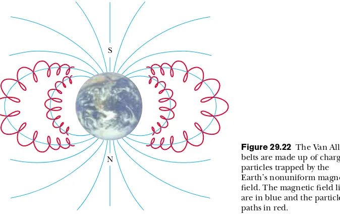
The Van Allen radiation belts consist of charged particles (mostly electrons and protons) surrounding the Earth in doughnut-shaped regions (Fig. 29.22). The parti-cles, trapped by the Earth’s nonuniform magnetic field, spiral around the field lines from pole to pole, covering the distance in just a few seconds. These particles originate mainly from the Sun, but some come from stars and other heavenly objects. For this reason, the particles are called cosmic rays.Most cosmic rays are deflected by the Earth’s magnetic field and never reach the atmosphere. However, some of the particles become trapped; it is these particles that make up the Van Allen belts. When the parti-cles are located over the poles, they sometimes collide with atoms in the atmosphere, causing the atoms to emit visible light. Such collisions are the origin of the beautiful Aurora Borealis, or Northern Lights, in the northern hemisphere and the Aurora Australis in the southern hemisphere. Auroras are usually confined to the polar regions because the Van Allen belts are nearest the Earth’s surface there. Occasionally, though, solar activity causes larger numbers of charged particles to enter the belts and significantly distort the normal magnetic field lines associated with the Earth. In these situations an aurora can sometimes be seen at lower latitudes.
29.5
Applications Involving Charged Particles
Moving in a Magnetic Field
A charge moving with a velocity vin the presence of both an electric field Eand a mag-netic field Bexperiences both an electric force qEand a magnetic force qv!B. The total force (called the Lorentz force) acting on the charge is
(29.16) F"qE'qv!B
Path of particle
+
Figure 29.21 A charged particle moving in a nonuniform
magneticfield (a magnetic bottle) spirals about the field and oscillates between the end points. The magnetic force exerted on the particle near either end of the bottle has a component that causes the particle to spiral back toward the center.
S
N
Figure 29.22 The Van Allen belts are made up of charged particles trapped by the Earth’s nonuniform magnetic field. The magnetic field lines are in blue and the particle paths in red.
S E C T I O N 2 9 . 5 • Applications Involving Charged Particles Moving in a Magnetic Field 911
Velocity Selector
In many experiments involving moving charged particles, it is important that the particles all move with essentially the same velocity. This can be achieved by applying a combina-tion of an electric field and a magnetic field oriented as shown in Figure 29.23. A uniform electric field is directed vertically downward (in the plane of the page in Fig. 29.23a), and a uniform magnetic field is applied in the direction perpendicular to the electric field (into the page in Fig. 29.23a). If qis positive and the velocity vis to the right, the magnetic force qv!Bis upward and the electric force qEis downward. When the magnitudes of the two fields are chosen so that qE"qvB, the particle moves in a straight horizontal line through the region of the fields. From the expression qE"qvB, we find that
(29.17)
Only those particles having speed vpass undeflected through the mutually perpendic-ular electric and magnetic fields. The magnetic force exerted on particles moving at speeds greater than this is stronger than the electric force, and the particles are deflected upward. Those moving at speeds less than this are deflected downward.
The Mass Spectrometer
A mass spectrometerseparates ions according to their mass-to-charge ratio. In one version of this device, known as the Bainbridge mass spectrometer,a beam of ions first passes through a velocity selector and then enters a second uniform magnetic field B0
that has the same direction as the magnetic field in the selector (Fig. 29.24). Upon
Active Figure 29.23 (a) A velocity selector. When a positively charged particle is moving with velocity vin the presence of a magnetic field directed into the page and an electric field directed downward, it experiences a downward electric force qEand an upward magnetic force qv!B.(b) When these forces balance, the particle moves in a horizontal line through the fields.
×
Active Figure 29.24 A mass spectrometer. Positively charged particles are sent first through a velocity selector and then into a region where the magnetic field B0causes the particles to move in a semicircular path and strike a detector array at P.
downward. From Equation 29.13, we can express the ratio m/qas
Using Equation 29.17, we find that
(29.18)
Therefore, we can determine m/qby measuring the radius of curvature and knowing the field magnitudes B, B0, and E. In practice, one usually measures the masses of
vari-ous isotopes of a given ion, with the ions all carrying the same charge q. In this way, the mass ratios can be determined even if qis unknown.
A variation of this technique was used by J. J. Thomson (1856–1940) in 1897 to measure the ratio e/mefor electrons. Figure 29.25a shows the basic apparatus he used. Electrons are accelerated from the cathode and pass through two slits. They then drift into a region of perpendicular electric and magnetic fields. The magnitudes of the two fields are first adjusted to produce an undeflected beam. When the magnetic field is turned off, the electric field produces a measurable beam deflection that is recorded on the fluorescent screen. From the size of the deflection and the measured values of
Eand B, the charge-to-mass ratio can be determined. The results of this crucial experi-ment represent the discovery of the electron as a fundaexperi-mental particle of nature.
m q "
rB0B
E m
q " rB0
v
Fluorescent coating
–
Slits Cathode
–
+ +
+
Deflection plates
Magnetic field coil
Deflected electron beam
Undeflected electron beam
(a)
Figure 29.25 (a) Thomson’s apparatus for measuring e/me. Electrons are accelerated from the cathode, pass through two slits, and are deflected by both an electric field and a magnetic field (directed perpendicular to the electric field). The beam of electrons then strikes a fluorescent screen. (b) J. J. Thomson (left)in the Cavendish Laboratory, University of Cambridge. The man on the right, Frank Baldwin Jewett, is a distant rela-tive of John W. Jewett, Jr., co-author of this text.
Bell T
elephone Labs/Courtesy of Emilio Segrè V
isual Archives
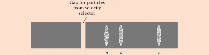
Quick Quiz 29.10
Three types of particles enter a mass spectrometer like the one shown in Figure 29.24. Figure 29.26 shows where the particles strike the detector array. Rank the particles that arrive at a, b, and cby speed and m/qratio.Figure 29.26 (Quick Quiz 29.10) Which particles have the highest speed and which have the highest ratio of m/q?
c b
a
Gap for particles from velocity
selector
S E C T I O N 2 9 . 5 • Applications Involving Charged Particles Moving in a Magnetic Field 913
The Cyclotron
A cyclotronis a device that can accelerate charged particles to very high speeds. The energetic particles produced are used to bombard atomic nuclei and thereby produce nuclear reactions of interest to researchers. A number of hospitals use cyclotron facili-ties to produce radioactive substances for diagnosis and treatment.
Both electric and magnetic forces have a key role in the operation of a cyclotron. A schematic drawing of a cyclotron is shown in Figure 29.27a. The charges move inside two semicircular containers D1and D2, referred to as dees, because of their shape like the letter D.A high-frequency alternating potential difference is applied to the dees, and a uniform magnetic field is directed perpendicular to them. A positive ion released at Pnear the center of the magnet in one dee moves in a semicircular path (indicated by the dashed red line in the drawing) and arrives back at the gap in a time interval T/2, where T is the time interval needed to make one complete trip around the two dees, given by Equation 29.15. The frequency of the applied potential differ-ence is adjusted so that the polarity of the dees is reversed in the same time interval during which the ion travels around one dee. If the applied potential difference is adjusted such that D2is at a lower electric potential than D1by an amount 0V, the ion accelerates across the gap to D2and its kinetic energy increases by an amount q0V. It then moves around D2in a semicircular path of greater radius (because its speed has increased). After a time interval T/2, it again arrives at the gap between the dees. By this time, the polarity across the dees has again been reversed, and the ion is given another “kick” across the gap. The motion continues so that for each half-circle trip around one dee, the ion gains additional kinetic energy equal to q0V. When the radius of its path is nearly that of the dees, the energetic ion leaves the system through the exit slit. Note that the operation of the cyclotron is based on the fact that Tis inde-pendent of the speed of the ion and of the radius of the circular path (Eq. 29.15).
We can obtain an expression for the kinetic energy of the ion when it exits the cyclotron in terms of the radius R of the dees. From Equation 29.13 we know that
v"qBR/m.Hence, the kinetic energy is
(29.19)
When the energy of the ions in a cyclotron exceeds about 20 MeV, relativistic effects come into play. (Such effects are discussed in Chapter 39.) We observe that T
increases and that the moving ions do not remain in phase with the applied potential
K"12mv2" q 2B2R2
2m
B
P
D1
D2
(a)
North pole of magnet Particle exits here Alternating ∆V
▲
PITFALL PREVENTION
29.1
The Cyclotron Is Not
State-of-the-Art
Technology
The cyclotron is important histori-cally because it was the first particle accelerator to achieve very high particle speeds. Cyclotrons are still in use in medical appli-cations, but most accelerators currently in research use are not cyclotrons. Research accelerators work on a different principle and are generally called synchrotrons.
Figure 29.27 (a) A cyclotron consists of an ion source at P, two dees D1and D2across which an alternating potential difference is applied, and a uniform magnetic field. (The south pole of the magnet is not shown.) The red dashed curved lines represent the path of the particles. (b) The first cyclotron, invented by E. O. Lawrence and M. S. Livingston in 1934.
Courtesy of Lawrence Berkeley Laboratory/University of California
difference. Some accelerators overcome this problem by modifying the period of the applied potential difference so that it remains in phase with the moving ions.
29.6
The Hall Effect
When a current-carrying conductor is placed in a magnetic field, a potential difference is generated in a direction perpendicular to both the current and the magnetic field. This phenomenon, first observed by Edwin Hall (1855–1938) in 1879, is known as the
Hall effect.It arises from the deflection of charge carriers to one side of the conductor as a result of the magnetic force they experience. The Hall effect gives information regarding the sign of the charge carriers and their density; it can also be used to measure the magnitude of magnetic fields.
The arrangement for observing the Hall effect consists of a flat conductor carrying a current Iin the xdirection, as shown in Figure 29.28. A uniform magnetic field Bis applied in the y direction. If the charge carriers are electrons moving in the negative
xdirection with a drift velocity vd, they experience an upward magnetic force FB"
qvd!B, are deflected upward, and accumulate at the upper edge of the flat conduc-tor, leaving an excess of positive charge at the lower edge (Fig. 29.29a). This accumula-tion of charge at the edges establishes an electric field in the conductor and increases until the electric force on carriers remaining in the bulk of the conductor balances the magnetic force acting on the carriers. When this equilibrium condition is reached, the electrons are no longer deflected upward. A sensitive voltmeter or potentiometer connected across the sample, as shown in Figure 29.29, can measure the potential difference—known as the Hall voltage0VH—generated across the conductor.
If the charge carriers are positive and hence move in the positive xdirection (for rightward current), as shown in Figures 29.28 and 29.29b, they also experience an upward magnetic force qvd!B. This produces a buildup of positive charge on the upper edge and leaves an excess of negative charge on the lower edge. Hence, the sign of the Hall voltage generated in the sample is opposite the sign of the Hall voltage resulting from the deflection of electrons. The sign of the charge carriers can therefore be determined from a measurement of the polarity of the Hall voltage.
In deriving an expression for the Hall voltage, we first note that the magnetic force exerted on the carriers has magnitude q vdB. In equilibrium, this force is balanced by the electric force q EH, where EH is the magnitude of the electric field due to the
charge separation (sometimes referred to as the Hall field). Therefore,
EH"vdB
qvdB"qEH
vd
y
vd
x z
a I
t
d
c
+ –
I
B
B FB
FB
S E C T I O N 2 9 . 6 • The Hall Effect 915
0
× × × × × × × × × × × × × × × × × × × × × × × × × × × × × × × × × × × × × × × × × × × ×
I I
+ + + + + + + + + – – – – – – – – –
(a) c
qvd×B –
qEH B
vd
a
∆VH
0
× × × × × × × × × × × × × × × × × × × × × × × × × × × × × × × × × × × × × × × × × × × ×
I I
– – – – – – – – – + + + + + + + + +
(b) c
qvd×B
qEH B
vd
a
+ ∆VH
Figure 29.29 (a) When the charge carriers in a Hall-effect apparatus are negative, the upper edge of the conductor becomes negatively charged, and cis at a lower electric potential than a. (b) When the charge carriers are positive, the upper edge becomes positively charged, and cis at a higher potential than a. In either case, the charge carri-ers are no longer deflected when the edges become sufficiently charged that there is a balance on the charge carriers between the electrostatic force q EHand the magnetic deflection force qvB.
If dis the width of the conductor, the Hall voltage is
(29.20)
Thus, the measured Hall voltage gives a value for the drift speed of the charge carriers if dand Bare known.
We can obtain the charge carrier density nby measuring the current in the sample. From Equation 27.4, we can express the drift speed as
(29.21)
where Ais the cross-sectional area of the conductor. Substituting Equation 29.21 into Equation 29.20, we obtain
(29.22)
Because A"td,where tis the thickness of the conductor, we can also express Equation 29.22 as
(29.23)
where RH"1/nqis the Hall coefficient.This relationship shows that a properly
cali-brated conductor can be used to measure the magnitude of an unknown magnetic field. Because all quantities in Equation 29.23 other than nqcan be measured, a value for the Hall coefficient is readily obtainable. The sign and magnitude of RHgive the sign
of the charge carriers and their number density. In most metals, the charge carriers are electrons, and the charge-carrier density determined from Hall-effect measurements is in good agreement with calculated values for such metals as lithium (Li), sodium (Na), copper (Cu), and silver (Ag), whose atoms each give up one electron to act as a current carrier. In this case, n is approximately equal to the number of conducting electrons per unit volume. However, this classical model is not valid for metals such as iron (Fe), bismuth (Bi), and cadmium (Cd) or for semiconductors. These discrepan-cies can be explained only by using a model based on the quantum nature of solids.
An interesting medical application related to the Hall effect is the electromagnetic blood flowmeter, first developed in the 1950s and continually improved since then. Imagine that we replace the conductor in Figure 29.29 with an artery carrying blood. The blood contains charged ions that experience electric and magnetic forces like the charge carriers in the conductor. The speed of flow of these ions can be related to the volume rate of flow of blood. Solving Equation 29.20 for the speed vdof the ions in
∆VH"
IB nqt "
RHIB
t
∆VH"
IBd nqA vd"
I nqA
∆VH"EHd"vdBd
the blood, we obtain
Thus, by measuring the voltage across the artery, the diameter of the artery, and the applied magnetic field, the speed of the blood can be calculated.
vd"
∆VH
Bd
Example 29.8 The Hall Effect for Copper
A rectangular copper strip 1.5 cm wide and 0.10 cm thick carries a current of 5.0 A. Find the Hall voltage for a 1.2-T magnetic field applied in a direction perpendicular to the strip.
Solution If we assume that one electron per atom is available for conduction, we can take the charge carrier density to be 8.49%1028 electrons/m3 (see Example 27.1). Substituting this value and the given data into Equation 29.23 gives
0.44 +V ∆VH"
" (5.0 A)(1.2 T)
(8.49%1028 m$3)(1.6%10$19 C)(0.001 0 m)
∆VH"
IB nqt
Such an extremely small Hall voltage is expected in good conductors. (Note that the width of the conductor is not needed in this calculation.)
What If? What if the strip has the same dimensions but is made of a semiconductor? Will the Hall voltage be smaller or larger?
Answer In semiconductors, nis much smaller than it is in metals that contribute one electron per atom to the current; hence, the Hall voltage is usually larger because it varies as the inverse of n. Currents on the order of 0.1 mA are gener-ally used for such materials. Consider a piece of silicon that has the same dimensions as the copper strip in this example and whose value for n is 1.0%1020 electrons/m3. Taking
B"1.2 T and I"0.10 mA, we find that 0VH"7.5 mV. A potential difference of this magnitude is readily measured.
The magnetic force that acts on a charge qmoving with a velocity vin a magnetic field Bis
(29.1)
The direction of this magnetic force is perpendicular both to the velocity of the parti-cle and to the magnetic field. The magnitude of this force is
(29.2)
where !is the smaller angle between vand B. The SI unit of Bis the tesla(T), where 1 T"1 N/A#m.
When a charged particle moves in a magnetic field, the work done by the magnetic force on the particle is zero because the displacement is always perpendicular to the direction of the force. The magnetic field can alter the direction of the particle’s velocity vector, but it cannot change its speed.
If a straight conductor of length Lcarries a current I, the force exerted on that conductor when it is placed in a uniform magnetic field Bis
(29.3)
where the direction of Lis in the direction of the current and !L!"L.
If an arbitrarily shaped wire carrying a current Iis placed in a magnetic field, the magnetic force exerted on a very small segment dsis
(29.4)
To determine the total magnetic force on the wire, one must integrate Equation 29.4, keeping in mind that both Band dsmay vary at each point. Integration gives for the
d FB"Ids!B FB"I L!B
FB" !q!vB sin ! FB"q v!B
S U M M A R Y
Take a practice test for this chapter by clicking on the Practice Test link at