AUTOMATIC CLUSTERING AND OPTIMIZED FUZZY LOGICAL
RELATIONSHIPS FOR MINIMUM LIVING NEEDS FORECASTING
Yusuf Priyo Anggodo1, Wayan Firdaus Mahmudy2
Faculty of Computer Science, Univesitas Brawijaya, Indonesia Email: [email protected], [email protected]
ABSTRACT
Forecasting of minimum living needs is useful for companies in financial planning next year. In this study, the firescasting is done using automatic clustering and optimized fuzzy logical relationships. Automatic clustering is used to form a sub-interval time series data. Particle swarm optimization is used to set and optimze interval values in fuzzy logical relationships. The data used as many as 11 years of historical data from 2005-2015. The optimal value of the test results obtained by the
p = 4, the number of iterations = 100, the number of particles = 45, a combination of
Vmin and Vmax = [-0.6, 0.6], as well as combinations Wmax and Wmin = [0, 4, 0 , 8]. These parameters values produce good forecasting results.
Keywords: minimum living needs, automatic clustering, particle swarm optimization, fuzzy logical relationships
1. INTRODUCTION
Minimum living needs is set in the regulation of the Minister of Manpower and Transmigration, namely "the need for decent living hereinafter abbreviated KHL is a standard requirement for a single worker or workers can live well physically to the needs of one (1) month". In addition to the articles 6 to 8 also stipulates that the KHM is used as a parameter for determining the minimum wage provinces and cities. From the information on the results of forecasting minimum necessities of life can be used as the design of the company's financial future.
Forecasting is usually done a lot of people to know the events that will occur in the future by looking at the events that have occurred previously (Chen et al, 2016). Such as forecasting temperature, precipitation, stock
items, earthquakes, etc. Forecasting
traditionally do not pay attention to the previous data and more qualitative not quantitative. On the problem of forecasting minimum life needs no studies when forecasting the minimum living needs will be beneficial for the company.
There are several methods of forecasting that uses quantitative approach, one of them is fuzzy logic (Fatyanosa & Mahmudy, 2016; Wahyuni, Mahmudy & Iriany, 2016). In addition there are other fuzzy model, the model of fuzzy time series Chen et al's more simple also be applied to predict the number of applicants at the University of Alabama (Chen and Tunawijaya, 2010). Forecasting methods developed by Chen et al's or so-called fuzzy logical relationship can produce good forecasting for time series data (Chen and Chen, 2011; Chen and Chen, 2015; Qiu et al, 2015; Cheng et al, 2015). Fuzzy logical relationship get an error lower than in previous studies. From the existing research can be concluded that the fuzzy logical relationship can solve the problems of forecasting.
Use of the method of automatic clustering effectively within the classification of previous data so that it can form a cluster with both (Chen and Tunawijaya, 2011; He and Tan, 2012; Saha and Bandyopadyay, 2013; Hung and Kang, 2014; Askari et al, 2015; Wang and Liu , 2015; Garcia and Flores, 2016). Deemed the use of automatic clustering greatly assist in forecasting to obtain the error value is lower. To improve forecasting results better optimization of the value interval on fuzzy logical relationships can be performed using particle swarm optimization giving an error that the lower (Chen and Kao, 2013; Cheng et al, 2016).
this study, the first to examine on the basis of fuzzy time series. The second classification data history minimum living needs using automatic clustering. Third optimization using particle swarm optimization interval. Fourth forecasting the minimum living needs using fuzzy logical relationships. Fifth calculate the error value using the Root Mean Squere Error (RMSE) forecasting results with actual data.
2. FUZZY TIME SERIES
Fuzzy time series is a representation of a fuzzy set. Fuzzy set is built based on the time series data of the KHM. A fuzzy set of data generated from the present into the current state and future year data into the next state. Fuzzy set which has been set used for forecasting the coming year.
2.1. Forecast Using Fuzzy Logical Relationships
In this section we will clarify the steps of forecasting methods fuzzy logical relationships by using automatic classification clustering, (Cheng et al, 2016) as follows:
Step 1: classifying the data using automatic clustering algorithm and optimize the value of the interval using the PSO.
Step 2: Assume there are n intervals, u1, u2, u3, ..., un. Then the form of fuzzy sets Ai,
where 1 ≤ i ≤ n, so that will be formed:
A1 = 1/u1 + 0.5/u2 + 0/u3 + 0/u4 + ... + 0/un-1 + 0/un,
A2 = 0.5/u1 + 1/u2 + 0.5/u3 + 0/u4 + ... + 0/un-1 + 0/un,
A3 = 0/u1 + 0.5/u2 + 1/u3 + 0.5/u4 + ... + 0/un-1 + 0/un,
. . .
An =0/u1 + 0/u2 + 0/u3 + 0/u4 + ... + 0.5/un-1 + 1/un.
Step 3: fuzzification every datum of historical data into fuzzy sets. If the datum is ui, where 1
≤ i ≤ n. So do fuzzification as Ai.
Step 4: building a relationship based on the fuzzy logical fuzzification step 3. If the fuzzification year t and t + 1 is Aj and Ak. So
fuzzy logical relationship that is built is Aj →
Ak, where Aj called the current state and the next state at the Ak as fuzzy logical relationship. From fuzzy logical relationship be grouped together, in which the same current state included in one group.
Step 5: forecasting using the following principles:
Principle 1: if fuzzification year t is Aj and there is a logical relationship in fuzzy fuzzy logical relationship group, with conditions:
Aj → Ak,
Thus, in forecasting the year t + 1 is mk, where mk is the midpoint of the interval uk and the maximum value of membership of fuzzy sets Ak Uk interval.
Principle 2: If fuzzification year t is Aj and no fuzzy logical ralationship in fuzzy logical relationship group, with conditions:
Aj → Ak¬1 (x1), Ak¬2 (x2), ... Ak¬p (xp)
So as to make forecasting year t + 1 using equation 1:
, (1) Where xi is the number of fuzzy logical relationships from Aj → Ak in fuzzy logical relationship group, 1 ≤ i ≤ n. mki is the
Principle 3: if fuzzification year t is Aj and there is a logical relationship in fuzzy fuzzy logical retlationship group, with conditions:
Aj → #
Where the value # is blank. Thus forecasting the year t + 1 is m¬j, where mj is the midpoint of the interval ui and a maximum value of membership of fuzzy sets Aj Uj interval.
2.2. Classification Of Data Using Automatic Clustering
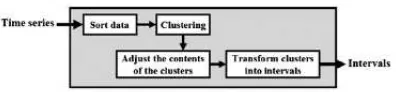
Figure 1.
Stages automatic clustering methods (Qiu et al, 2015)Here are the steps automatic clustering algorithm (Wang and Liu, 2015; Chen and Tunawijaya, 2015):
Step 1: The first sort ascending numerical data, assuming no similar data.
d1, d2, d3,. , , , di. , , ,dn.
Then calculate avarage_diff using equation 2:
avarage_diff = ∑
, (2)
avarage_diff which is the average of the data numberik and d1, d1, ...,dn. is the numerical
data that has been sorted.
Step 2: Take the first numerical data (ie the smallest datum) to be placed to the current cluster or need to create a new cluster based on the following principles:
Principle 1: assume the current cluster is the first cluster and there is only one datum that d1 and d2 is considered that datum adjacent to d1, shown as follows:
{d1}, d2, d3, ..., di, ..., dn.
If avarage_diff≤ d2-d1, d2 then input into the current cluster consisting d1, if it does
not create a new cluster consisting d2.
Principle 2: assume that the current cluster is not the first cluster and dj is the datum
only in the current cluster. Assume dk is
adjacent to the datum datum datum dj and
is the largest in the antecedent of a cluster, shown as follows:
{d1}, . . . , {...,di},{dj}, dk, . . . , dn.
If the dk-dj ≤ avarage_diff and dk - dj≤ dj -
di, then input to a cluster owned dk dj, if it
does not create a new cluster consisting dk.
Principle 3: assume that the current cluster is not the first cluster and assume that in a datum the current cluster. Assume that datum adadalah dj nearest to.
{d1}, . . . , {....},{. . . , di}, dj, . . . , dn.
If dj-di ≤ avarage_diff and dj-di ≤ cluster_diff, then dj input into clusters
consisting di. If it does not create a new
cluster for dj. Cluster_diff calculation
shown in equation 3.
cluster_diff = ∑
, (3)
cluster_diff which is the average of the current cluster and c1, c2, ... cn is the data
in the current cluster.
Step 3: based on the clarification step 2, according to the contents corresponding cluster following principles:
Principle 1: if the cluster there are more than two datum, then maintain the smallest and largest datum and datum remove the others.
Principle 2: If the cluster there are two datum, then maintain it all.
Principle 3: If the cluster has only one datum dq, then add the datum to the value dq - avarage_diff and dq + avarage_diff
into clusters. But also must adjust to the following situations:
Situation 1: if the first cluster, then remove dq - avarage_diff and maintain
dq.
Situation 2: if the cluster Last post, then remove avarage_diff + dq and
maintain dq.
Situation 3: if dq - avarage_diff smaller
than the smallest value in the antecedent cluster datum, then the third principle does not apply.
Step 4: assume the results of step 3 as follows:
{d1, d2}, {d3, d4}, {d5, d6}, . . ., {dr}, {ds, dt}, . . .
, {dn-1, dn}.
Changing the cluster results into an adjacent cluster sub-step through the following:
4.1 The first cluster fox {d1, d2} to the
interval [d1, d2).
4.2 if the current interval [di, dj) and the
current cluster {dk, dl}, then:
(1) if the dj ≥ dk, then the shape of an
interval [dj, dl). interval [dj, dl) is now the
current interval and the next cluster {dm,
dn} be the current cluster.
(2) if di < dk, then change the current
cluster {dk, dl} to the interval [dk, dl) and
create a new interval [dj, dk) on the
becomes current and next interval cluster {dm, dn} be the current cluster. If now the
current interval [di, dj) and the current
cluster is {df}, then change the current
interval [di, dj) be [di, dk). Now [di, dk) is
the current interval and next interval becomes current inteval.
4.3 repeat sub-steps 4.1 and 4.2 until all cluster into intervals.
Step 5: results of step 4 for the interval into sub-intervals p, where p≥ 1.
2.3. Interval Optimization Using PSO
The concept of PSO algorithm is quite simple and effective in for finding solutions of complex problems (Novitasari, Cholissodin & Mahmudy, 2016; Mahmudy 2014), PSO algorithm model the best solution search by activities of particles moving in the search space, the position of the particle is a representation of the solution represented by the cost. Cost value obtained from the calculation error forecasting results using the RMSE (Cheng et al, 2016). PSO main concept is every particle has a speed which is calculated based pbest and gbest and coefficient values was raised at random. Each to shift the position of each particle must update the value of pbest, gbest, as well as the speed of each particle.
The process of the PSO algorithm in the optimization objective function in accordance with the problems. The first initializes particles presenting the solution of problems. Both do the calculation of the value of cost for each particle. The third did the best position value updates of each particle or particles or pbest and overall gbest. Fourth calculate the speed of each particle, the particle velocity will determine the direction of movement of the particle's position. The fifth did displacement particle positions and do repair to sort in ascending value of the particle, the first iteration randomly generated for the next iteration obtained by equation 4.
vit+1 = w.vi + c1.r1(pbit– xit )+ c2.r2(gbt– xit), (4)
which vi shows the particle velocity i, t is the
iteration time, w is the weight of inertia, ci is
the coefficient of particles (cognitive = 1, social = 2), ri is a random value in the interval
[0,1], xi the value of the position of the particle
i, gb t
value the best solution on the particle i and iteration t, and the best overall solution value gbt particle at iteration t. Once the updated value of the speed, the next step is to change the position of each particle using the equation 5.
xi t+1
= xi t
+ vi t+1
, (5)
Each iteration changes inertia weight value shown in equation 6.
w = wmin + (wmax– wmin)
, (6)
tmax is the maximum iteration value has
diinsialisasi beginning before PSO do, t is an ongoing iteration. wmax and wmin a minimum
and maximum weight diinsialisasi previously. Updates the value of w in equation 6 usually called time varying Inertia Weight (TVIW).
In the PSO algorithm implementation is sometimes found fast moving particles, the particles have a tendency to come out as a result of the search space limit. Hence, to control the exploitation of the particles need to be limits on the minimum and maximum speed or so-called velocity clamping (Marini and Walczak, 2015). The calculation of the speed limit is shown in equation 7.
vmax = k , (7)
Where vmax shows the value of the maximum
speed, k generated at random intervals (0, 1], whereas xmax and xmin respectively the smallest
and largest value of minimum living needs. Limitation of speed or threshold that is used as follows:
ifvi t+1
> vmax then vi t+1
= vmax ifvi
t+1
< vmax then vi t+1
= - vmax
3. EXPERIMENTAL RESULT
living needs. For testing the PSO performed 10 times. Use of this because stotastic PSO algorithm, the best result of the average value.
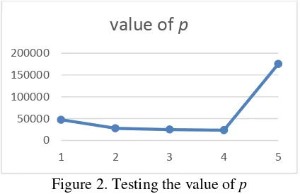
3.1. Testing The Value of P
The first will be tested on automatic clustering p values shown in Figure 2.
Figure 2. Testing the value of p
Figure 2 shows the value of p = 4 RMSE worth 23404,944 and when the value of p = 5 RMSE values increase. Based on this it does not conduct further testing of the p value for a value of more than 5.
3.2. Testing of Iterations
Testing iteration aims to see the value of the best iterations on this issue. These initial conditions include a parameter p = 4, the number of particles = 5, Wmax = 0.9, Wmin = 0.1, c1 = 1, c2 = 1. Figure 3 shows the results of
testing the number of iterations.
Figure 3 shows the number of iterations of 100 had a value of cost (RMSE) from the bottom at 22065.574096827. Can be seen in the increasing number of iterations does not mean the lower the cost is because the PSO algorithm is an algorithm stotastic or random nature.
3.3. Testing the Number of Particle
Testing the numberof particles aimed to look at the value of the number of particles the best on this issue. These initial conditions include a parameter p = 4, the number of iterations = 100, Wmax = 0.9, Wmin = 0.1, c1 =
1, c2 = 1. Figure 4 shows the results of testing
the number of particles.
Figure 4. Testing the number of particles
Figure 4 shows the number of particles 45 provides a value that is equal to the lowest cost 22036.208233097. On the number of particles after 45 value higher cost, so that on this issue the best particle number is 45.
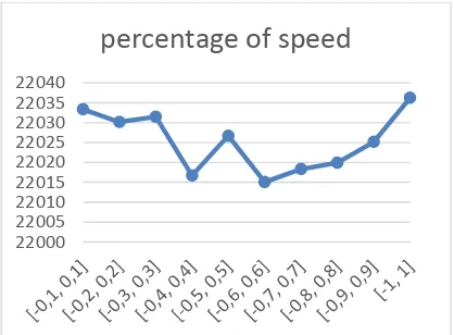
3.4. Testing Percentage of Speed
Testing the percentage of speed or Vmin and Vmax aims to know the value of a percentage of the dynamic range of the velocity of particles in PSO resulting combination with interval fuzzy logical relationships are optimal. These initial conditions include a parameter p = 4, the number of iterations = 100, the number of particles = 45, Wmax = 0.9, Wmin = 0.1, c1 = 1,
c2 = 1. Figure 5 shows the percentage of the
speed test results.
0 50000 100000 150000 200000
1 2 3 4 5
value of p
22020 22040 22060 22080
5 10 15 20 25 30 35 40 45 50
number of particles
21900 22000 22100 22200 22300
10 30 50 70 90 110 130 150
iterations
Figure 5. Testing the percentage of speed
Figure 5 shows a combination of the best value Vmin and Vmax is [-0.6, 0,6]. In the combination produced the lowest cost value is equal 22015.075310004.
3.5. Testing Value of Wmin and Wmax
Testing the value of Wmin and Wmax to get the best combination. These initial conditions include a parameter p = 4, the number of iterations = 100, the number of particles = 45, Vmin = -0.6, Vmax = 0.6, c1 = 1,
c2 = 1. Figure 6 shows the results of testing the
value Wmin and Wmax.
Figure 6 shows the best combination of value
Wmin and Wmax is [0.4, 0.8] for
22006.341736784
.
3.6. Testing using the Best Parameter
This section will compare the results of forecasting the results of forecasting using
automatic clustering, fuzzy logical
relationships (ACFLR) with p = 4 while the forecasting results using automatic clustering,
particle swarm optimization, and fuzzy logical relationships with the parameter value p = 4, the number of iterations = 100, the number of particles = 45, the percentage of Vmax = 0.6, the percentage of Vmin = -0.6, Wmin = 0.4, Wmax = 0.8, c1 = 1 and c2 = 1 shown in Figure
7.
Figure 7. Compare the result of forecasting
Figure 7 shows the results of data comparison between the actual with ACPSOFLR and
ACFLR, where ACPSOFLR forecasting
results closer to the actual data with RMSE value of 22006.34154 while ACFLR has RMSE value of 23404.9442.
4. CONCLUSION
Fuzzy logical Relatioships Particle swarm optimization is very helpful to optimize the value of the interval on fuzzy logical relationships that get results RMSE values were lower. Automatic clustering in classifying time series data to establish the interval. The best parameter values so as to produce the optimal value, among others, p = 4, the number of iterations = 100, the number of particles = 45, the percentage of speed = [-0.6, 0.6], the value Wmin and Wmax = [0.4, 0.8 ].
Further research can be applied this method for forecasting other data are more numerous and optimizing the parameters of fuzzy logical relationships resulting in smaller RMSE values.
5. REFERENCES
ANGGODO, YP & MAHMUDY, WF 2016, 'Peramalan Butuhan Hidup Minimum Menggunakan Automatic Clustering dan Fuzzy Logical Relationship ', Jurnal Teknologi Informasi dan Ilmu Komputer, vol. 3, no. 2, pp. 94-102.
22000 22005 22010 22015 22020 22025 22030 22035 22040
percentage of speed
0 200000 400000 600000 800000 1000000
2006 2007 2008 2009 2010 2011 2012 2013 2014 2015
Aktual ACFLR ACPSOFLR
21990 21995 22000 22005 22010 22015 22020 22025 22030 22035
[0,2 0,7]
[0,2 0,8]
[0,2 0,9]
[0,3 0,7]
[0,3 0,8]
[0,3 0,9]
[0,4 0,7]
[0,4 0,8]
[0,4 0,9] Wmin andWmax
ASKARI, S., MONTAZERIN, N. & ZARANDI, M. H. F. 2015. A clustering
based forecasting algorithm for
multivariable fuzzy time series using
linear combinations of indepent
variables. Applied Soft Computing, 35, 151-160.
CHEN, S. M. & CHEN, C. D. 2011. Handling forecasting problems based on high-order fuzzy logical relationships. Expert Systems with Applications, 38, 3856-3864.
CHEN, S. M. & CHEN, S. W. 2015. Fuzzy forecasting based on two-factors second-order fuzzy-trend logical relationship group and the probabilites of tren of fuzzy logical relatonships. IEEE Transactions on Cybernetics, Vol 45, No. 3.
CHEN, S. M. & KAO, P. Y. 2013. TAIEX forecasting based on fuzzy time series, particle swarm optimazation techniques
and support vector machines.
Information Sciences, 247, 62-71. CHEN, S. M. & TUNAWIJAYA, K. 2011.
Multivariate fuzzy forecasting based on fuzzy time series and automatic clustering technique. Expert System with Applications, 38, 10594-10605.
CHENG, S. H., CHEN, S. M. & JIAN, W. S. 2015. A novel fuzzy time series forecasting method based on fuzzy logical relationships and similarity
measures. IEEE International
Conference on Systems, Man, and Cybernetics, 978(1), 4799-8697.
CHENG S. H., CHEN, S. M. & JIAN, W. S. 2016. Fuzzy time series forecasting based on fuzzy logical relationships and
similarity measures. Information
Sciences, 327, 272-287.
FATYANOSA, TN & MAHMUDY, WF 2016, Implementation of Real Coded Genetic Fuzzy System for Rainfall Forecasting, International Conference on Sustainable Information Engineering and Technology (SIET), Malang, 17 October, Fakultas Ilmu Komputer, Universitas Brawijaya, pp. 24-33.
GARCIA, A. J. & FLORES, W. G. 2016. Automatic clustering using nature-inspired metaheuristics : a survey. Applied Soft Computing, 41, 192-213. HE, H. & TAN, Y. 2012. A Two-stage genetic
algorithm for automatic clustering. Neurcomputing, 81, 49-59.
MAHMUDY, WF 2014, Optimasi part type selection and machine loading problems
pada FMS menggunakan metode
particle swarm optimization, Konferensi Nasional Sistem Informasi (KNSI), STMIK Dipanegara, Makassar, 27 Februari - 1 Maret, pp. 1718-1723. MARINI, F. & WALCZAK, B. 2015. Paticle
swarm optimization (PSO). A tutorial. Chemometrics and Intellegent Laboratory Systems, 149, 153-165. NOVITASARI, D, CHOLISSODIN, I &
MAHMUDY, WF 2016, Hybridizing PSO With SA for Optimizing SVR Applied to Software Effort Estimation, Telkomnika (Telecommunication Computing Electronics and Control), vol. 14, no. 1, pp. 245-253.
QIU, W., ZHANG, P. & WANG, Y. 2015. Fuzzy time series forecasting model
based on automatic clustering
techniques and generalized fuzzy logical
relationship. Hindawi Publishing
Corporation Mathematical Problems in Engineering, 962597.
SAHA, S. & BANDYOPADHYAY, S. 2013. A generalized automatic clustering algorithm in a multiobjective famework. Applied Soft Computing, 13, 89-108. WAHYUNI, I, MAHMUDY, WF & IRIANY,
A 2016, Rainfall Prediction in Tengger Region Indonesia using Tsukamoto Fuzzy Inference System, International Conference on Information Technology, Information Systems and Electrical Engineering (ICITISEE), Yogyakarta, Indonesia, 23-24 August 2016, pp. 130-135.
WANG, W. DAN LIU, X., 2015. Fuzzy
forecasting based on automatic