Academic.Press.Elasticity.Theory.Applications.and.Numerics

(1)

(2)

(3)

ELASTICITY

(4)

(5)

ELASTICITY

Theory, Applications, and Numerics

MARTIN H. SADD

Professor, University of Rhode Island

Department of Mechanical Engineering and Applied Mechanics Kingston, Rhode Island

AMSTERDAM . BOSTON

.

HEIDELBERG

.

LONDON

.

NEW YORK OXFORD . PARIS

.

SAN DIEGO

.

SAN FRANCISCO

.

SINGAPORE

(6)

Elsevier Butterworth–Heinemann

200 Wheeler Road, Burlington, MA 01803, USA Linacre House, Jordan Hill, Oxford OX2 8DP, UK

No part of this publication may be reproduced, stored in a retrieval system, or transmitted in

any form or by any means, electronic, mechanical, photocopying, recording, or otherwise, without the prior written permission of the publisher.

Permissions may be sought directly from Elsevier’s Science & Technology Rights Department in Oxford, UK: phone: (þ44) 1865 843830, fax: (þ44) 1865 853333, e-mail: permissions@elsevier.com.uk. You may also complete your request on-line via the Elsevier homepage (http://www.elsevier.com), by selecting ‘‘Customer Support’’ and then ‘‘Obtaining Permissions.’’

Recognizing the importance of preserving what has been written, Elsevier prints its books on acid-free paper whenever possible.

Library of Congress Cataloging-in-Publication Data

ISBN 0-12-605811-3

British Library Cataloguing-in-Publication Data

A catalogue record for this book is available from the British Library. (Application submitted)

For information on all Butterworth–Heinemann publications visit our Web site at www.bh.com

04 05 06 07 08 09 10 10 9 8 7 6 5 4 3 2 1

(7)

Preface

This text is an outgrowth of lecture notes that I have used in teaching a two-course sequence in theory of elasticity. Part I of the text is designed primarily for the first course, normally taken by beginning graduate students from a variety of engineering disciplines. The purpose of the first course is to introduce students to theory and formulation and to present solutions to some basic problems. In this fashion students see how and why the more fundamental elasticity model of deformation should replace elementary strength of materials analysis. The first course also provides the foundation for more advanced study in related areas of solid mechanics. More advanced material included in Part II has normally been used for a second course taken by second- and third-year students. However, certain portions of the second part could be easily integrated into the first course.

So what is the justification of my entry of another text in the elasticity field? For many years, I have taught this material at several U.S. engineering schools, related industries, and a government agency. During this time, basic theory has remained much the same; however, changes in problem solving emphasis, research applications, numerical/computational methods, and engineering education pedagogy have created needs for new approaches to the subject. The author has found that current textbook titles commonly lack a concise and organized presentation of theory, proper format for educational use, significant applications in contemporary areas, and a numerical interface to help understand and develop solutions.

(8)

of MATLAB, one of the most popular engineering software packages. This software is used throughout the text for applications such as: stress and strain transformation, evaluation and plotting of stress and displacement distributions, finite element calculations, and making comparisons between strength of materials, and analytical and numerical elasticity solutions. With numerical and graphical evaluations, application problems become more interesting and useful for student learning.

Text Contents

The book is divided into two main parts; the first emphasizes formulation details and elemen-tary applications. Chapter 1 provides a mathematical background for the formulation of elasticity through a review of scalar, vector, and tensor field theory. Cartesian index tensor notation is introduced and is used throughout the formulation sections of the book. Chapter 2 covers the analysis of strain and displacement within the context of small deformation theory. The concept of strain compatibility is also presented in this chapter. Forces, stresses, and equilibrium are developed in Chapter 3. Linear elastic material behavior leading to the generalized Hook’s law is discussed in Chapter 4. This chapter also includes brief discussions on non-homogeneous, anisotropic, and thermoelastic constitutive forms. Later chapters more fully investigate anisotropic and thermoelastic materials. Chapter 5 collects the previously derived equations and formulates the basic boundary value problems of elasticity theory. Displacement and stress formulations are made and general solution strategies are presented. This is an important chapter for students to put the theory together. Chapter 6 presents strain energy and related principles including the reciprocal theorem, virtual work, and minimum potential and complimentary energy. Two-dimensional formulations of plane strain, plane stress, and anti-plane strain are given in Chapter 7. An extensive set of solutions for specific two-dimensional problems are then presented in Chapter 8, and numerous MATLAB applica-tions are used to demonstrate the results. Analytical soluapplica-tions are continued in Chapter 9 for the Saint-Venant extension, torsion, and flexure problems. The material in Part I provides the core for a sound one-semester beginning course in elasticity developed in a logical and orderly manner. Selected portions of the second part of this book could also be incorporated in such a beginning course.

(9)

The Subject

Elasticity is an elegant and fascinating subject that deals with determination of the stress, strain, and displacement distribution in an elastic solid under the influence of external forces. Following the usual assumptions of linear, small-deformation theory, the formulation estab-lishes a mathematical model that allows solutions to problems that have applications in many engineering and scientific fields. Civil engineering applications include important contribu-tions to stress and deflection analysis of structures including rods, beams, plates, and shells. Additional applications lie in geomechanics involving the stresses in such materials as soil, rock, concrete, and asphalt. Mechanical engineering uses elasticity in numerous problems in analysis and design of machine elements. Such applications include general stress analysis, contact stresses, thermal stress analysis, fracture mechanics, and fatigue. Materials engineering uses elasticity to determine the stress fields in crystalline solids, around dislocations and in materials with microstructure. Applications in aeronautical and aerospace engineering include stress, fracture, and fatigue analysis in aerostructures. The subject also provides the basis for more advanced work in inelastic material behavior including plasticity and viscoe-lasticity, and to the study of computational stress analysis employing finite and boundary element methods.

Elasticity theory establishes a mathematical model of the deformation problem, and this requires mathematical knowledge to understand the formulation and solution procedures. Governing partial differential field equations are developed using basic principles of con-tinuum mechanics commonly formulated in vector and tensor language. Techniques used to solve these field equations can encompass Fourier methods, variational calculus, integral transforms, complex variables, potential theory, finite differences, finite elements, etc. In order to prepare students for this subject, the text provides reviews of many mathematical topics, and additional references are given for further study. It is important that students are adequately prepared for the theoretical developments, or else they will not be able to under-stand necessary formulation details. Of course with emphasis on applications, we will concen-trate on theory that is most useful for problem solution.

(10)

Exercises and Web Support

Of special note in regard to this text is the use of exercises and the publisher’s web site, www.books.elsevier.com. Numerous exercises are provided at the end of each chapter for homework assignment to engage students with the subject matter. These exercises also provide an ideal tool for the instructor to present additional application examples during class lectures. Many places in the text make reference to specific exercises that work out details to a particular problem. Exercises marked with an asterisk (*) indicate problems requiring numerical and plotting methods using the suggested MATLAB software. Solutions to all exercises are provided on-line at the publisher’s web site, thereby providing instructors with considerable help in deciding on problems to be assigned for homework and those to be discussed in class. In addition, downloadable MATLAB software is also available to aid both students and instructors in developing codes for their own particular use, thereby allowing easy integration of the numerics.

Feedback

The author is keenly interested in continual improvement of engineering education and strongly welcomes feedback from users of this text. Please feel free to send comments concerning suggested improvements or corrections via surface or e-mail (sadd@egr.uri.edu). It is likely that such feedback will be shared with text user community via the publisher’s web site.

Acknowledgments

Many individuals deserve acknowledgment for aiding the successful completion of this textbook. First, I would like to recognize the many graduate students who have sat in my elasticity classes. They are a continual source of challenge and inspiration, and certainly influenced my efforts to find a better way to present this material. A very special recognition goes to one particular student, Ms. Qingli Dai, who developed most of the exercise solutions and did considerable proofreading. Several photoelastic pictures have been graciously pro-vided by our Dynamic Photomechanics Laboratory. Development and production support from several Elsevier staff was greatly appreciated. I would also like to acknowledge the support of my institution, the University of Rhode Island for granting me a sabbatical leave to complete the text. Finally, a special thank you to my wife, Eve, for being patient with my extended periods of manuscript preparation.

This book is dedicated to the late Professor Marvin Stippes of the University of Illinois, who first showed me the elegance and beauty of the subject. His neatness, clarity, and apparent infinite understanding of elasticity will never be forgotten by his students.

(11)

About the Author

(15)

(16)

(17)

1 Mathematical Preliminaries

Similar to other field theories such as fluid mechanics, heat conduction, and electromagnetics, the study and application of elasticity theory requires knowledge of several areas of applied mathematics. The theory is formulated in terms of a variety of variables including scalar, vector, and tensor fields, and this calls for the use of tensor notation along with tensor algebra and calculus. Through the use of particular principles from continuum mechanics, the theory is developed as a system of partial differential field equations that are to be solved in a region of space coinciding with the body under study. Solution techniques used on these field equations commonly employ Fourier methods, variational techniques, integral transforms, complex variables, potential theory, finite differences, and finite and boundary elements. Therefore, to develop proper formulation methods and solution techniques for elasticity problems, it is necessary to have an appropriate mathematical background. The purpose of this initial chapter is to provide a background primarily for the formulation part of our study. Additional review of other mathematical topics related to problem solution technique is provided in later chapters where they are to be applied.

1.1 Scalar, Vector, Matrix, and Tensor Definitions

(18)

mass density scalar¼r

wheree1,e2,e3 are the usual unit basis vectors in the coordinate directions. Thus, scalars,

vectors, and matrices are specified by one, three, and nine components, respectively. The formulation of elasticity problems not only involves these types of variables, but also incorporates additional quantities that require even more components to characterize. Because of this, most field theories such as elasticity make use of atensor formalismusing index notation. This enables efficient representation of all variables and governing equations using a single standardized scheme. The tensor concept is defined more precisely in a later section, but for now we can simply say that scalars, vectors, matrices, and other higher-order variables can all be represented by tensors of various orders. We now proceed to a discussion on the notational rules of order for the tensor formalism. Additional information on tensors and index notation can be found in many texts such as Goodbody (1982) or Chandrasekharaiah and Debnath (1994).

1.2 Index Notation

Index notation is a shorthand scheme whereby a whole set of numbers (elements or compon-ents) is represented by a single symbol with subscripts. For example, the three numbers a1,a2,a3 are denoted by the symbolai, where indexiwill normally have the range 1, 2, 3.

In a similar fashion,aij represents the nine numbersa11,a12,a13,a21,a22,a23,a31,a32,a33.

Although these representations can be written in any manner, it is common to use a scheme related to vector and matrix formats such that

ai¼

In the matrix format,a1j represents the first row, whileai1 indicates the first column. Other

columns and rows are indicated in similar fashion, and thus the first index represents the row, while the second index denotes the column.

In general a symbol a_ij...k with N distinct indices represents 3N distinct numbers. It should be apparent that ai and aj represent the same three numbers, and likewise aij and amn signify the same matrix. Addition, subtraction, multiplication, and equality of index symbols are defined in the normal fashion. For example, addition and subtraction are given by

(19)

lai¼

la1

la2

la3

2

4 3

5,laij¼

la11 la12 la13

la21 la22 la23

la31 la32 la33

2

4

3

5 (1:2:3)

The multiplication of two symbols with different indices is calledouter multiplication,and a simple example is given by

aibj¼

a1b1 a1b2 a1b3

a2b1 a2b2 a2b3

a3b1 a3b2 a3b3

2

4

3

5 (1:2:4)

The previous operations obey usual commutative, associative, and distributive laws, for example:

ai_þbi_¼bi_þai aijbk ¼bkaij

aiþ(biþci)¼(aiþbi)þci ai(bjkcl)_¼(aibjk)cl

aij(bkþck)¼aijbkþaijck

(1:2:5)

Note that the simple relations ai¼bi and aij¼bij imply that a1¼b1, a2¼b2,. . .and

a11¼b11,a12¼b12, . . . However, relations of the form ai¼bj oraij¼bkl have ambiguous

meaning because the distinct indices on each term are not the same, and these types of expressions are to be avoided in this notational scheme. In general, the distinct subscripts on all individual terms in an equation should match.

It is convenient to adopt the convention that if a subscript appears twice in the same term, thensummationover that subscript from one to three is implied; for example:

aii¼X

3

i¼1

aii¼a11þa22þa33

aijbj¼ X

3

j¼1

aijbj¼ai1b1þai2b2þai3b3

(1:2:6)

It should be apparent that aii¼ajj¼akk¼. . ., and therefore the repeated subscripts or indices are sometimes calleddummysubscripts. Unspecified indices that are not repeated are calledfreeordistinctsubscripts. The summation convention may be suspended by underlining one of the repeated indices or by writingno sum. The use of three or more repeated indices in the same term (e.g.,aiii oraiijbij) has ambiguous meaning and is to be avoided. On a given symbol, the process of setting two free indices equal is calledcontraction. For example,aiiis obtained from aij by contraction on i and j. The operation of outer multiplication of two indexed symbols followed by contraction with respect to one index from each symbol generates aninner multiplication; for example,aijbjk is an inner product obtained from the outer productaijbmkby contraction on indicesjandm.

A symbolaij_...m...n...kis said to besymmetricwith respect to index pairmnif

(20)

while it isantisymmetricorskewsymmetricif

aij_...m...n...k¼ aij...n...m...k (1:2:8)

Note that ifaij_...m...n...k is symmetric inmnwhilebpq...m...n...r is antisymmetric inmn, then the product is zero:

aij_...m...n...kbpq...m...n...r¼0 (1:2:9)

A useful identity may be written as

aij¼1

2(aijþaji)þ 1

2(aijaji)¼a(ij)þa[ij] (1:2:10) The first terma(ij)¼1=2(aijþaji) is symmetric, while the second terma[ij]¼1=2(aijaji) is

antisymmetric, and thus an arbitrary symbolaijcan be expressed as the sum of symmetric and antisymmetric pieces. Note that ifaijis symmetric, it has only six independent components. On the other hand, ifaijis antisymmetric, its diagonal termsaii(no sum oni) must be zero, and it has only three independent components. Note that sincea[ij]has only three independent

compon-ents, it can be related to a quantity with a single index, for example,ai(see Exercise 1-14).

1.3 Kronecker Delta and Alternating Symbol

A useful special symbol commonly used in index notational schemes is theKronecker delta defined by

dij_¼ 1,if i¼j(no sum) 0,if i6¼j

¼

1 0 0 0 1 0 0 0 1 2

4

3

5 (1:3:1)

Within usual matrix theory, it is observed that this symbol is simply the unit matrix. Note that the Kronecker delta is a symmetric symbol. Particular useful properties of the Kronecker delta include the following:

dij¼dji dii¼3,dii¼1 dijaj_¼ai,dijai_¼aj dijajk¼aik,djkaik¼aij dijaij¼aii,dijdij¼3

(1:3:2)

Another useful special symbol is thealternatingorpermutation symboldefined by

eijk¼ þ

1, if ijkis an even permutation of 1, 2, 3

1, if ijkis an odd permutation of 1, 2, 3 0, otherwise

(

(1:3:3)

Consequently, e123¼e231¼e312¼1,e321¼e132¼e213¼ 1,e112¼e131¼e222¼. . .¼0.

(21)

equal to1, and all others are 0. The alternating symbol is antisymmetric with respect to any pair of its indices.

This particular symbol is useful in evaluating determinants and vector cross products, and the determinant of an arrayaijcan be written in two equivalent forms:

det[aij]¼ jaijj ¼

where the first index expression represents the row expansion, while the second form is the column expansion. Using the property

eijkepqr¼

another form of the determinant of a matrix can be written as

det[aij]¼ 1

6eijkepqraipajqakr (1:3:6)

1.4 Coordinate Transformations

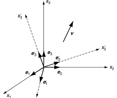
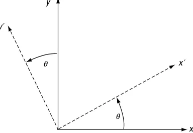
It is convenient and in fact necessary to express elasticity variables and field equations in several different coordinate systems (see Appendix A). This situation requires the development of particular transformation rules for scalar, vector, matrix, and higher-order variables. This concept is fundamentally connected with the basic definitions of tensor variables and their related tensor transformation laws. We restrict our discussion to transformations only between Cartesian coordinate systems, and thus consider the two systems shown in Figure 1-1. The two Cartesian frames (x1,x2,x3) and (x01,x02,x03) differ only by orientation, and the unit basis vectors

(22)

LetQijdenote the cosine of the angle between thex0_i-axis and thexj-axis:

Qij¼cos (x0_i,xj) (1:4:1)

Using this definition, the basis vectors in the primed coordinate frame can be easily expressed in terms of those in the unprimed frame by the relations

e0₁¼Q11e1þQ12e2þQ13e3

e02¼Q21e1þQ22e2þQ23e3

e0₃¼Q31e1þQ32e2þQ33e3

(1:4:2)

or in index notation

e0_i¼Qijej (1:4:3)

Likewise, the opposite transformation can be written using the same format as

ei¼Qjie0_j (1:4:4)

Now an arbitrary vectorvcan be written in either of the two coordinate systems as

v¼v1e1þv2e2þv3e3¼viei

¼v0₁e01þv02e02þv03e03¼v0ie0i

(1:4:5)

Substituting form (1.4.4) into (1:4:5)1gives

v¼viQjie0_j

but from (1:4:5)2,v¼v0je0j, and so we find that

v0_i_¼Qijvj (1:4:6)

In similar fashion, using (1.4.3) in (1:4:5)2gives

vi¼Qjiv0_j (1:4:7)

Relations (1.4.6) and (1.4.7) constitute the transformation laws for the Cartesian components of a vector under a change of rectangular Cartesian coordinate frame. It should be understood that under such transformations, the vector is unaltered (retaining original length and orienta-tion), and only its components are changed. Consequently, if we know the components of a vector in one frame, relation (1.4.6) and/or relation (1.4.7) can be used to calculate components in any other frame.

The fact that transformations are being made only between orthogonal coordinate systems places some particular restrictions on the transformation or direction cosine matrixQij. These can be determined by using (1.4.6) and (1.4.7) together to get

(23)

From the properties of the Kronecker delta, this expression can be written as

dikvk¼QjiQjkvk or (QjiQjkdik)vk¼0

and since this relation is true for all vectorsvk, the expression in parentheses must be zero, giving the result

QjiQjk ¼dik (1:4:9)

In similar fashion, relations (1.4.6) and (1.4.7) can be used to eliminatevi(instead ofv0i) to get

QijQkj¼dik (1:4:10)

Relations (1.4.9) and (1.4.10) comprise the orthogonality conditions that Qij must satisfy. Taking the determinant of either relation gives another related result:

det[Qij]¼ 1 (1:4:11)

Matrices that satisfy these relations are called orthogonal, and the transformations given by (1.4.6) and (1.4.7) are therefore referred to as orthogonal transformations.

1.5 Cartesian Tensors

Scalars, vectors, matrices, and higher-order quantities can be represented by a general index notational scheme. Using this approach, all quantities may then be referred to as tensors of different orders. The previously presented transformation properties of a vector can be used to establish the general transformation properties of these tensors. Restricting the transformations to those only between Cartesian coordinate systems, the general set of transformation relations for various orders can be written as

a0_¼a, zero order (scalar)

a0_i_¼Qipap,Wrst order (vector)

a0_ij¼QipQjqapq, second order (matrix) a0ijk¼QipQjqQkrapqr, third order a0_ijkl_¼QipQjqQkrQlsapqrs, fourth order

.. .

a0_ijk_..._m¼QipQjqQkr Qmtapqr_...tgeneral order

(1:5:1)

(24)

tensor. The alternating symboleijkis found to be the third-order isotropic form. The fourth-order case (Exercise 1-9) can be expressed in terms of products of Kronecker deltas, and this has important applications in formulating isotropic elastic constitutive relations in Section 4.2.

The distinction between the components and the tensor should be understood. Recall that a vectorvcan be expressed as

v¼v1e1þv2e2þv3e3¼viei

¼v0₁e0₁þv0₂e0₂þv0₃e0₃¼v0_ie0_i (1:5:2)

In a similar fashion, a second-order tensorAcan be written

A¼A11e1e1þA12e1e2þA13e1e3

þA21e2e1þA22e2e2þA23e2e3

þA31e3e1þA32e3e2þA33e3e3

¼Aijeiej¼A0_ije0ie0j

(1:5:3)

and similar schemes can be used to represent tensors of higher order. The representation used in equation (1.5.3) is commonly called dyadic notation,and some authors write the dyadic productseiejusing atensor productnotationeiej. Additional information on dyadic notation can be found in Weatherburn (1948) and Chou and Pagano (1967).

Relations (1.5.2) and (1.5.3) indicate that any tensor can be expressed in terms of compon-ents in any coordinate system, and it is only the componcompon-ents that change under coordinate transformation. For example, the state of stress at a point in an elastic solid depends on the problem geometry and applied loadings. As is shown later, these stress components are those of a second-order tensor and therefore obey transformation law (1:5:1)3. Although the

com-ponents of the stress tensor change with the choice of coordinates, the stress tensor (represent-ing the state of stress) does not.

An important property of a tensor is that if we know its components in one coordinate system, we can find them in any other coordinate frame by using the appropriate transform-ation law. Because the components of Cartesian tensors are representable by indexed symbols, the operations of equality, addition, subtraction, multiplication, and so forth are defined in a manner consistent with the indicial notation procedures previously discussed. The terminology tensorwithout the adjectiveCartesianusually refers to a more general scheme in which the coordinates are not necessarily rectangular Cartesian and the transformations between coordin-ates are not always orthogonal. Such general tensor theory is not discussed or used in this text.

EXAMPLE 1-1: Transformation Examples

The components of a first- and second-order tensor in a particular coordinate frame are given by

ai¼

1 4 2 2

4 3

5,aij¼

1 0 3 0 2 2 3 2 4 2

4

3

(25)

EXAMPLE 1-1: Transformation Examples–

Cont’d

Determine the components of each tensor in a new coordinate system found through a rotation of 608 (p=6 radians) about the x3-axis. Choose a counterclockwise rotation

when viewing down the negativex3-axis (see Figure 1-2).

The original and primed coordinate systems shown in Figure 1-2 establish the angles be-tween the various axes. The solution starts by determining the rotation matrix for this case:

Qij¼

The transformation for the vector quantity follows from equation (1:5:1)2:

a0_i¼Qijaj¼

and the second-order tensor (matrix) transforms according to (1:5:1)3:

a0_ij_¼QipQjqapq_¼

where [ ]Tindicates transpose (defined in Section 1.7). Although simple transformations can be worked out by hand, for more general cases it is more convenient to use a computational scheme to evaluate the necessary matrix multiplications required in the transformation laws (1.5.1). MATLAB software is ideally suited to carry out such calculations, and an example program to evaluate the transformation of second-order tensors is given in Example C-1 in Appendix C.

x₃

(26)

1.6 Principal Values and Directions for Symmetric

Second-Order Tensors

Considering the tensor transformation concept previously discussed, it should be apparent that there might exist particular coordinate systems in which the components of a tensor take on maximum or minimum values. This concept is easily visualized when we consider the components of a vector shown in Figure 1-1. If we choose a particular coordinate system that has been rotated so that the x3-axis lies along the direction of the vector, then

the vector will have componentsv¼{0, 0,jvj}. For this case, two of the components have been reduced to zero, while the remaining component becomes the largest possible (the total magnitude).

This situation is most useful for symmetric second-order tensors that eventually represent the stress and/or strain at a point in an elastic solid. The direction determined by the unit vector nis said to be aprincipal directionoreigenvectorof the symmetric second-order tensoraijif there exists a parameterlsuch that

aijnj¼lni (1:6:1)

where l is called the principal value or eigenvalueof the tensor. Relation (1.6.1) can be rewritten as

(aijldij)nj¼0

and this expression is simply a homogeneous system of three linear algebraic equations in the unknownsn1,n2,n3. The system possesses a nontrivial solution if and only if the determinant

of its coefficient matrix vanishes, that is:

det[aijldij]¼0

Expanding the determinant produces a cubic equation in terms ofl:

det[aijldij]¼ l3þIal2IIalþIIIa¼0 (1:6:2)

The scalarsIa,IIa, andIIIaare called thefundamental invariantsof the tensoraij, and relation (1.6.2) is known as thecharacteristic equation. As indicated by their name, the three invariants do not change value under coordinate transformation. The roots of the characteristic equation determine the allowable values forl, and each of these may be back-substituted into relation (1.6.1) to solve for the associated principal directionn.

Under the condition that the componentsaijare real, it can be shown that all three roots l1,l2,l3of the cubic equation (1.6.2) must be real. Furthermore, if these roots are distinct, the

(27)

principal directions and at most three distinct principal values that are the roots of the characteristic equation. By denoting the principal directions n(1)_,_n(2)_,_n(3)_{corresponding to}

the principal valuesl1,l2,l3, three possibilities arise:

1. All three principal values distinct; thus, the three corresponding principal directions are unique (except for sense).

2. Two principal values equal (l16¼l2¼l3); the principal directionn(1)is unique

(except for sense), and every direction perpendicular ton(1)is a principal direction associated withl2,l3.

3. All three principal values equal; every direction is principal, and the tensor is isotropic, as per discussion in the previous section.

Therefore, according to what we have presented, it is always possible to identify a right-handed Cartesian coordinate system such that each axis lies along the principal directions of any given symmetric second-order tensor. Such axes are called the principal axes of the tensor. For this case, the basis vectors are actually the unit principal directions {n(1)_,_n(2)_,_n(3)_{}, and it can be shown that with respect to principal axes the tensor reduces to}

the diagonal form

aij_¼

l1 0 0

0 l2 0

0 0 l3

2

4

3

5 (1:6:4)

Note that the fundamental invariants defined by relations (1.6.3) can be expressed in terms of the principal values as

Ia¼l1þl2þl3

IIa¼l1l2þl2l3þl3l1

IIIa_¼l1l2l3

(1:6:5)

The eigenvalues have important extremal properties. If we arbitrarily rank the principal values such thatl1>l2>l3, thenl1will be the largest of all possible diagonal elements, whilel3

will be the smallest diagonal element possible. This theory is applied in elasticity as we seek the largest stress or strain components in an elastic solid.

EXAMPLE 1-2: Principal Value Problem

Determine the invariants and principal values and directions of the following symmetric second-order tensor:

aij¼

2 0 0

0 3 4

0 4 3 2

4

3

5

The invariants follow from relations (1.6.3)

(28)

EXAMPLE 1-2: Principal Value Problem–

Cont’d

The characteristic equation then becomes

det[aijldij]¼ l3þ2l2þ25l50¼0

)(l2)(l225)¼0

;l1¼5,l2¼2,l3¼ 5

Thus, for this case all principal values are distinct. For thel1¼5 root, equation (1.6.1) gives the system

3n(1)₁ _¼0

. In similar fashion, the other two principal directions are found to ben(2)¼ e1,n(3)¼ (e22e3)=

ffiffiffi 5

p

. It is easily verified that these directions are mutually orthogonal. Figure 1-3 illustrates their direc-tions with respect to the given coordinate system, and this establishes the right-handed principal coordinate axes (x0₁,x0₂,x0₃). For this case, the transformation matrixQijdefined by (1.4.1) becomes

Notice the eigenvectors actually form the rows of theQ-matrix.

x₃

(29)

EXAMPLE 1-2: Principal Value Problem–

Cont’d

Using this in the transformation law (1:5:1)3, the components of the given second-order

tensor become

This result then validates the general theory given by relation (1.6.4) indicating that the tensor should take on diagonal form with the principal values as the elements.

Only simple second-order tensors lead to a characteristic equation that is factorable, thus allowing solution by hand calculation. Most other cases normally develop a general cubic equation and a more complicated system to solve for the principal directions. Again particular routines within the MATLAB package offer convenient tools to solve these more general problems. Example C-2 in Appendix C provides a simple code to determine the principal values and directions for symmetric second-order tensors.

1.7 Vector, Matrix, and Tensor Algebra

Elasticity theory requires the use of many standard algebraic operations among vector, matrix, and tensor variables. These operations include dot and cross products of vectors and numerous matrix/tensor products. All of these operations can be expressed efficiently using compact tensor index notation. First, consider some particular vector products. Given two vectorsaand b, with Cartesian componentsaiandbi, thescalarordot productis defined by

ab¼a1b1þa2b2þa3b3¼aibi (1:7:1)

Because all indices in this expression are repeated, the quantity must be a scalar, that is, a tensor of order zero. The magnitude of a vector can then be expressed as

jaj ¼(aa)1=2¼(aiai)1=2 (1:7:2) Thevectororcross productbetween two vectorsaandbcan be written as

ab¼

whereeiare the unit basis vectors for the coordinate system. Note that the cross product gives a vector resultant whose components areeijkajbk. Another common vector product is thescalar triple productdefined by

abc¼

(30)

Aa¼[A]{a}¼Aijaj_¼ajAij aTA¼{a}T[A]¼aiAij¼Aijai

(1:7:5)

whereaT _{denotes the} _transpose,_{and for a vector quantity this simply changes the column} matrix (31) into a row matrix (13). Note that each of these products results in a vector resultant. These types of expressions generally involve various inner products within the index notational scheme, and as noted, once the summation index is properly specified, the order of listing the product terms does not change the result. We will encounter several different combinations of products between two matricesAandB:

AB¼[A][B]_¼AijBjk ABT¼AijBkj ATB¼AjiBjk tr(AB)¼AijBji

tr(ABT)¼tr(ATB)¼AijBij

(1:7:6)

whereAT indicates thetransposeandtrAis thetraceof the matrix defined by

AT_ij¼Aji

trA_¼Aii¼A11þA22þA33

(1:7:7)

Similar to vector products, once the summation index is properly specified, the results in (1.7.6) do not depend on the order of listing the product terms. Note that this does not imply thatAB¼BA, which is certainly not true.

1.8 Calculus of Cartesian Tensors

Most variables within elasticity theory are field variables, that is, functions depending on the spatial coordinates used to formulate the problem under study. For time-dependent problems, these variables could also have temporal variation. Thus, our scalar, vector, matrix, and general tensor variables are functions of the spatial coordinates (x1,x2,x3). Because many

elasticity equations involve differential and integral operations, it is necessary to have an understanding of the calculus of Cartesian tensor fields. Further information on vector differen-tial and integral calculus can be found in Hildebrand (1976) and Kreyszig (1999).

The field concept for tensor components can be expressed as

a¼a(x1,x2,x3)¼a(xi)¼a(x)

ai¼ai(x1,x2,x3)¼ai(xi)¼ai(x)

aij_¼aij(x1,x2,x3)¼aij(xi)¼aij(x)

.. .

It is convenient to introduce thecomma notationfor partial differentiation:

a,i¼ @

@xia,ai,j¼ @

(31)

It can be shown that if the differentiation index is distinct, the order of the tensor is increased by one. For example, the derivative operation on a vectorai_,jproduces a second-order tensor or matrix given by

ai_,j¼

Using Cartesian coordinates (x,y,z), consider the directional derivative of a scalar field functionfwith respect to a directions:

df

Note that the unit vector in the direction ofscan be written as

n¼dx

Therefore, the directional derivative can be expressed as the following scalar product:

df

ds¼n rrrf (1:8:1) whererrrf is called thegradientof the scalar functionfand is defined by

rr

and the symbolic vector operatorrrris called thedel operator

r

These and other useful operations can be expressed in Cartesian tensor notation. Given the scalar fieldfand vector fieldu, the following common differential operations can be written in index notation:

Laplacian of a Vectorr2_u

¼ui,kkei

(32)

Iffandcare scalar fields anduandvare vector fields, several useful identities exist:

Each of these identities can be easily justified by using index notation from definition relations (1.8.4).

Next consider some results from vector/tensor integral calculus. We simply list some theorems that have later use in the development of elasticity theory.

1.8.1 Divergence or Gauss Theorem

LetSbe a piecewise continuous surface bounding the region of spaceV. If a vector fielduis continuous and has continuous first derivatives inV, then

ð ð

wherenis the outer unit normal vector to surfaceS. This result is also true for tensors of any order, that is:

LetSbe an open two-sided surface bounded by a piecewise continuous simple closed curveC. Ifuis continuous and has continuous first derivatives onS, then

þ

where the positive sense for the line integral is for the regionSto lie to the left as one traverses curveC andnis the unit normal vector toS. Again, this result is also valid for tensors of arbitrary order, and so

(33)

It can be shown that both divergence and Stokes theorems can be generalized so that the dot product in (1.8.6) and/or (1.8.8) can be replaced with a cross product.

1.8.3 Green’s Theorem in the Plane

Applying Stokes theorem to a planar domainSwith the vector field selected asu¼fe1þge2

gives the result

ð ð

S @g @x

@f @y

dxdy¼

ð

C

(fdxþgdy) (1:8:10)

Further, special choices with eitherf _¼0 org_¼0 imply

ð ð

S @g @xdxdy¼

ð

C gnxds,

ð ð

S @f @ydxdy¼

ð

C

fnyds (1:8:11)

1.8.4 Zero-Value Theorem

Letfij_...kbe a continuous tensor field of any order defined in an arbitrary regionV. If the integral offij_...k overVvanishes, thenfij...k must vanish inV, that is:

ð ð ð

V

fij_...kdV¼0)fij_...k¼02V (1:8:12)

1.9 Orthogonal Curvilinear Coordinates

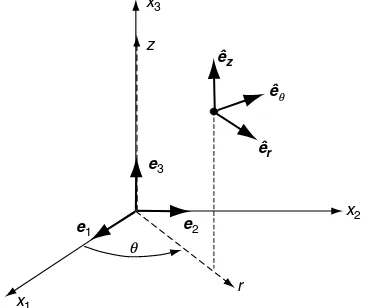
Many applications in elasticity theory involve domains that have curved boundary surfaces, commonly including circular, cylindrical, and spherical surfaces. To formulate and develop solutions for such problems, it is necessary to use curvilinear coordinate systems. This requires redevelopment of some previous results in orthogonal curvilinear coordinates. Before pursuing these general steps, we review the two most common curvilinear systems, cylindrical and spherical coordinates. The cylindrical coordinate system shown in Figure 1-4 uses (r,y,z)

e₂ e₃

e₁

x₃

x₁

x₂

r

q

z

ê_z

ê_r ê_q

(34)

coordinates to describe spatial geometry. Relations between the Cartesian and cylindrical systems are given by

x1¼rcosy,x2¼siny,x3¼z

r¼

ffiffiffiffiffiffiffiffiffiffiffiffiffiffiffi x2

1þx22

q

,y_¼tan1x2 x1

,z¼x3

(1:9:1)

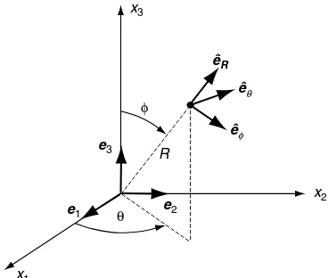
The spherical coordinate system is shown in Figure 1-5 and uses (R,f,y) coordinates to describe geometry. The relations between Cartesian and spherical coordinates are

x1¼Rcosysinf,x2¼Rsinysinf,x3¼Rcosf

R¼

ffiffiffiffiffiffiffiffiffiffiffiffiffiffiffiffiffiffiffiffiffiffiffiffi x2

1þx22þx23

q

,f_¼cos1 ffiffiffiffiffiffiffiffiffiffiffiffiffiffiffiffiffiffiffiffiffiffiffiffix3 x2

1þx22þx23

p ,y¼tan 1x2

x1

(1:9:2)

The unit basis vectors for each of these curvilinear systems are illustrated in Figures 4 and 1-5. These represent unit tangent vectors along each of the three orthogonal coordinate curves.

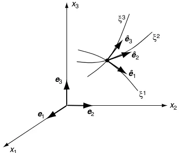
Although primary use of curvilinear systems employs cylindrical and spherical coordinates, we briefly present a general discussion valid for arbitrary coordinate systems. Consider the general case in which three orthogonal curvilinear coordinates are denoted byx1_,_x2_,_x3_{, while}

the Cartesian coordinates are defined byx1_,_x2_,_x3 _{(see Figure 1-6). We assume there exist}

invertible coordinate transformations between these systems specified by

xm_¼xm(x1_,_x2_,_x3_),_xm

¼xm(x1,x2,x3) (1:9:3)

In the curvilinear system, an arbitrary differential length in space can be expressed by

(ds)2¼(h1dx1)2þ(h2dx2)2þ(h3dx3)2 (1:9:4)

whereh1,h2,h3are calledscale factorsthat are in general nonnegative functions of position.

Letek be the fixed Cartesian basis vectors andee^k the curvilinear basis (see Figure 1-6). By

e₃

e₂ e₁

x₃

x₁

x₂ R

ê_R

êq

êf

θ φ

(35)

using similar concepts from the transformations discussed in Section 1.5, the curvilinear basis can be expressed in terms of the Cartesian basis as

^

It follows from (1.9.5) that the quantity

Qk_r¼_h1

r @xk

@xr, (no sum onr) (1:9:7)

represents the transformation tensor giving the curvilinear basis in terms of the Cartesian basis. This concept is similar to the transformation tensorQijdefined by (1.4.1) that is used between Cartesian systems.

Thephysical componentsof a vector or tensor are simply the components in a local set of Cartesian axes tangent to the curvilinear coordinate curves at any point in space. Thus, by using transformation relation (1.9.7), the physical components of a tensor a in a general curvilinear system are given by

e₂

(36)

a<ij...k>¼QpiQ q j Q

s

kapq...s (1:9:8)

where apq_...s are the components in a fixed Cartesian frame. Note that the tensor can be expressed in either system as

a¼aij_...keiej ek

¼a<ij...k>ee^i^eej ee^k

(1:9:9)

Because many applications involve differentiation of tensors, we must consider the differenti-ation of the curvilinear basis vectors. The Cartesian basis systemekis fixed in orientation and therefore @ek=@xj¼@ek=@xj¼0. However, derivatives of the curvilinear basis do not in

general vanish, and differentiation of relations (1.9.5) gives the following results:

@ee^m

Using these results, the derivative of any tensor can be evaluated. Consider the first derivative of a vectoru:

The last term can be evaluated using (1.9.10), and thus the derivative ofucan be expressed in terms of curvilinear components. Similar patterns follow for derivatives of higher-order tensors. All vector differential operators of gradient, divergence, curl, and so forth can be expressed in any general curvilinear system by using these techniques. For example, the vector differen-tial operator previously defined in Cartesian coordinates in (1.8.3) is given by

r ¼^ee1

and this leads to the construction of the other common forms:

Gradient of a Scalar_r_r_rf _¼ee^1

Laplacian of a Scalarr2_f

(37)

Gradient of a Vectorru¼X

Laplacian of a Vector_r2_u

¼ X

It should be noted that these forms are significantly different from those previously given in relations (1.8.4) for Cartesian coordinates. Curvilinear systems add additional terms not found in rectangular coordinates. Other operations on higher-order tensors can be developed in a similar fashion (see Malvern 1969, app. II). Specific transformation relations and field equa-tions in cylindrical and spherical coordinate systems are given in Appendices A and B. Further discussion of these results is taken up in later chapters.

EXAMPLE 1-3: Polar Coordinates

Consider the two-dimensional case of a polar coordinate system as shown in Figure 1-7. The differential length relation (1.9.4) for this case can be written as

(ds)2_¼(dr)2_þ(rdy)2

and thush1¼1 andh2¼r. By using relations (1.9.5) or simply by using the geometry

shown in Figure 1-7,

^

(38)

EXAMPLE 1-3: Polar Coordinates–

Cont’d

The basic vector differential operations then follow to be

r simply pass through and operate on each of the individual components as in the Cartesian case. Additional terms are generated because of the curvature of the particular coordinate system. Similar relations can be developed for cylindrical and spherical coordinate systems (see Exercises 1-15 and 1-16).

The material reviewed in this chapter is used in many places for formulation develop-ment of elasticity theory. Throughout the entire text, notation uses scalar, vector, and tensor formats depending on the appropriateness to the topic under discussion. Most of the general formulation procedures in Chapters 2 through 5 use tensor index notation, while later chapters commonly use vector and scalar notation. Additional review of mathe-matical procedures for problem solution is supplied in chapter locations where they are applied.

References

Chandrasekharaiah DS, Debnath L:Continuum Mechanics, Academic Press, Boston, 1994.

Chou PC, Pagano NJ: Elasticity—Tensor, Dyadic and Engineering Approaches, D. Van Nostrand, Princeton, NJ, 1967.

Goodbody AM:Cartesian Tensors: With Applications to Mechanics, Fluid Mechanics and Elasticity, Ellis Horwood, New York, 1982.

Hildebrand FB:Advanced Calculus for Applications, 2nd ed, Prentice Hall, Englewood Cliffs, NJ, 1976. Kreyszig E:Advanced Engineering Mathematics, 8th ed, John Wiley, New York, 1999.

Malvern LE:Introduction to the Mechanics of a Continuous Medium, Prentice Hall, Englewood Cliffs, NJ, 1969.

(39)

Exercises

1-1. For the given matrix and vector

aij¼

1 1 1 0 4 2 0 1 1 2

4

3

5,bi¼ 1 0 2 2

4 3

5

compute the following quantities:aii,aijaij,aijajk,aijbj,aijbibj,bibj,bibi. For each quantity, point out whether the result is a scalar, vector, or matrix. Note thataijbjis actually the matrix product [a]{b}, whileaijajk is the product [a][a].

1-2. Use the decomposition result (1.2.10) to expressaijfrom Exercise 1-1 in terms of the sum of symmetric and antisymmetric matrices. Verify thata(ij)anda[ij]satisfy the conditions

given in the last paragraph of Section 1.2.

1-3. Ifaijis symmetric andbijis antisymmetric, prove in general that the productaijbijis zero. Verify this result for the specific case by using the symmetric and antisymmetric terms from Exercise 1-2.

1-4. Explicitly verify the following properties of the Kronecker delta:

dijaj¼ai dijajk_¼aik

1-5. Formally expand the expression (1.3.4) for the determinant and justify that either index notation form yields a result that matches the traditional form for det[aij].

1-6. Determine the components of the vectorbiand matrixaijgiven in Exercise 1-1 in a new coordinate system found through a rotation of 458(p=4 radians) about thex1-axis. The

rotation direction follows the positive sense presented in Example 1-1.

1-7. Consider the two-dimensional coordinate transformation shown in Figure 1-7. Through the counterclockwise rotationy, a new polar coordinate system is created. Show that the transformation matrix for this case is given by

Qij¼ cosy siny siny cosy

Ifbi¼ b1

b2

,aij¼ a11

a12

a21

a22

are the components of a first- and second-order tensor in the

x1,x2system, calculate their components in the rotated polar coordinate system.

1-8. Show that the second-order tensoradij, whereais an arbitrary constant, retains its form under any transformationQij. This form is then an isotropic second-order tensor.

1-9. The most general form of a fourth-order isotropic tensor can be expressed by

adijdklþbdikdjlþgdildjk

wherea,b, andgare arbitrary constants. Verify that this form remains the same under the general transformation given by (1.5.1)5.

(40)

1-11. Determine the invariants, principal values, and directions of the matrix

Use the determined principal directions to establish a principal coordinate system, and, following the procedures in Example 1-2, formally transform (rotate) the given matrix into the principal system to arrive at the appropriate diagonal form.

1-12*. A second-order symmetric tensor field is given by

aij¼

Using MATLAB (or similar software), investigate the nature of the variation of the principal values and directions over the interval 1x12. Formally plot the variation

of the absolute value of each principal value over the range 1x12.

1-13. For the Cartesian vector field specified by

u¼x1e1þx1x2e2þ2x1x2x3e3

calculater rr u,rr r u,r2_u_,_r_r_r_u_,_tr₍_r_r_r_u₎_:

1-14. Thedual vector aiof an antisymmetric second-order tensoraijis defined by ai¼ 1=2eijkajk. Show that this expression can be inverted to getajk¼ eijkai. 1-15. Using index notation, explicitly verify the three vector identities (1.8.5)2,6,9.

1-16. Extend the results found in Example 1-3, and determine the forms ofrrrf,rrr u,r2_f_,

andrrr ufor a three-dimensional cylindrical coordinate system (see Figure 1-4). 1-17. For the spherical coordinate system (R,f,y) in Figure 1-5, show that

h1¼1,h2¼R,h3¼Rsinf

and the standard vector operations are given by

(41)

2 Deformation: Displacements and Strains

We begin development of the basic field equations of elasticity theory by first investigating the kinematics of material deformation. As a result of applied loadings, elastic solids will change shape or deform, and these deformations can be quantified by knowing the displacements of material points in the body. The continuum hypothesis establishes a displacement field at all points within the elastic solid. Using appropriate geometry, particular measures of deformation can be constructed leading to the development of the strain tensor. As expected, the strain components are related to the displacement field. The purpose of this chapter is to introduce the basic definitions of displacement and strain, establish relations between these two field quantities, and finally investigate requirements to ensure single-valued, continuous displace-ment fields. As appropriate for linear elasticity, these kinematical results are developed under the conditions of small deformation theory. Developments in this chapter lead to two funda-mental sets of field equations: the strain-displacement relations and the compatibility equa-tions. Further field equation development, including internal force and stress distribution, equilibrium and elastic constitutive behavior, occurs in subsequent chapters.

2.1 General Deformations

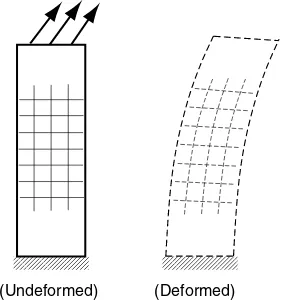
Under the application of external loading, elastic solids deform. A simple two-dimensional cantilever beam example is shown in Figure 2-1. The undeformed configuration is taken with the rectangular beam in the vertical position, and the end loading displaces material points to the deformed shape as shown. As is typical in most problems, the deformation varies from point to point and is thus said to benonhomogenous. A superimposed square mesh is shown in the two configurations, and this indicates how elements within the material deform locally. It is apparent that elements within the mesh undergo extensional and shearing deformation. An elastic solid is said to be deformed or strained when therelative displacementsbetween points in the body are changed. This is in contrast torigid-body motionwhere the distance between points remains the same.

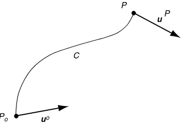
In order to quantify deformation, consider the general example shown in Figure 2-2. In the undeformed configuration, we identify two neighboring material points Poand P connected with

(42)

undeformed and deformed configurations can be significantly different, and a distinction between these two configurations must be maintained leading to Lagrangian and Eulerian descriptions; see, for example, Malvern (1969) or Chandrasekharaiah and Debnath (1994). However, since we are developing linear elasticity, which uses only small deformation theory, the distinction between undeformed and deformed configurations can be dropped.

Using Cartesian coordinates, define the displacement vectors of points Poand P to beuoand

u, respectively. Since P and Poare neighboring points, we can use a Taylor series expansion

around point Poto express the components ofuas

u¼uoþ@u

@xrxþ @u @yryþ

@u @zrz

v¼voþ@v

@xrxþ @v @yryþ

@v @zrz

w¼woþ@w

@xrxþ @w

@yryþ @w

@zrz

(2:1:1)

(Undeformed) (Deformed)

FIGURE 2-1 Two-dimensional deformation example.

P

Po

r _r

(Undeformed) (Deformed)

′ ′

′

(43)

Note that the higher-order terms of the expansion have been dropped since the components ofr are small. The change in the relative position vectorrcan be written as

Dr¼r0r¼uuo (2:1:2)

and using (2.1.1) gives

Drx¼@u

or in index notation

Dri_¼ui_,jrj (2:1:4)

The tensorui,jis called thedisplacement gradient tensor,and may be written out as

ui,j¼

From relation (1.2.10), this tensor can be decomposed into symmetric and antisymmetric parts as

The tensoreijis called thestrain tensor,while!ijis referred to as therotation tensor. Relations (2.1.4) and (2.1.6) thus imply that for small deformation theory, the change in the relative position vector between neighboring points can be expressed in terms of asumof strain and rotation components. Combining relations (2.1.2), (2.1.4), and (2.1.6), and choosingri¼dxi, we can also write the general result in the form

ui¼uo_iþeijdxjþ!ijdxj (2:1:8)

(44)

be associated with the rotation tensor such that!i¼ 1=2eijk!jk. Using this definition, it is found that

!1¼!32¼

1 2

@u3

@x2

@u2

@x3

!2¼!13¼

1 2

@u1

@x3

@u3

@x1

!3¼!21¼

1 2

@u2

@x1

@u1

@x2

(2:1:9)

which can be expressed collectively in vector format asv¼(1=2)(r u). As is shown in the next section, these components represent rigid-body rotation of material elements about the coordinate axes. These general results indicate that the strain deformation is related to the strain tensoreij, which in turn is a related to the displacement gradients. We next pursue a more geometric approach and determine specific connections between the strain tensor components and geometric deformation of material elements.

2.2 Geometric Construction of Small Deformation Theory

Although the previous section developed general relations for small deformation theory, we now wish to establish a more geometrical interpretation of these results. Typically, elasticity variables and equations are field quantities defined at each point in the material continuum. However, particular field equations are often developed by first investigating the behavior of infinitesimal elements (with coordinate boundaries), and then a limiting process is invoked that allows the element to shrink to a point. Thus, consider the common deformational behavior of a rectangular element as shown in Figure 2-3. The usual types of motion include rigid-body rotation and extensional and shearing deformations as illustrated. Rigid-body motion does not contribute to the strain field, and thus also does not affect the stresses. We therefore focus our study primarily on the extensional and shearing deformation.

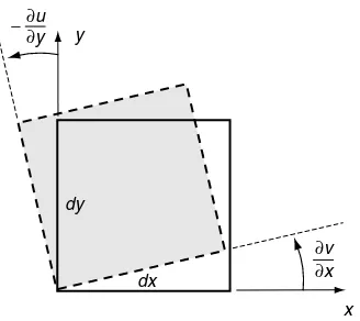
Figure 2-4 illustrates the two-dimensional deformation of a rectangular element with original dimensions dx by dy. After deformation, the element takes a rhombus form as shown in the dotted outline. The displacements of various corner reference points are indicated

(Rigid Body Rotation) (Undeformed Element)

(Horizontal Extension) (Vertical Extension) (Shearing Deformation)

(45)

in the figure. Reference pointAis taken at location (x,y), and the displacement components of this point are thus u(x,y) and v(x,y). The corresponding displacements of point B are u(xþdx,y) andv(xþdx,y), and the displacements of the other corner points are defined in an analogous manner. According to small deformation theory, u(xþdx,y)u(x,y)þ (@u=@x)dx, with similar expansions for all other terms.

Thenormal orextensional strain componentin a direction nis defined as the change in length per unit length of fibers oriented in the n-direction. Normal strain is positive if fibers increase in length and negative if the fiber is shortened. In Figure 2-4, the normal strain in thex direction can thus be defined by

ex _¼A 0_B0_AB

AB

From the geometry in Figure 2-4,

A0B0¼

where, consistent with small deformation theory, we have dropped the higher-order terms. Using these results and the fact thatAB¼dx, the normal strain in thex-direction reduces to

ex_¼@u

@x (2:2:1)

In similar fashion, the normal strain in they-direction becomes

ey¼@v

@y (2:2:2)

A second type of strain is shearing deformation, which involves angles changes (see Figure 2-3). Shear strain is defined as the change in angle between two originally orthogonal

u(x,y)

(46)

directions in the continuum material. This definition is actually referred to as theengineering shear strain. Theory of elasticity applications generally use a tensor formalism that requires a shear strain definition corresponding to one-half the angle change between orthogonal axes; see previous relation (2:1:7)1. Measured in radians, shear strain is positive if the right angle

between the positive directions of the two axes decreases. Thus, the sign of the shear strain depends on the coordinate system. In Figure 2-4, the engineering shear strain with respect to thex-andy-directions can be defined as

g_xy_¼p 2 ﬀC

0_A0_B0_¼_a_þ_b

For small deformations,atanaandbtanb, and the shear strain can then be expressed as

gxy¼

where we have again neglected higher-order terms in the displacement gradients. Note that each derivative term is positive if linesABandACrotate inward as shown in the figure. By simple interchange ofxandyanduandv, it is apparent thatg_xy_¼g_yx.

By considering similar behaviors in the y-zand x-z planes, these results can be easily extended to the general three-dimensional case, giving the results:

ex¼@u

Thus, we define three normal and three shearing strain components leading to a total of six independent components that completely describe small deformation theory. This set of equations is normally referred to as thestrain-displacement relations. However, these results are written in terms of the engineering strain components, and tensorial elasticity theory prefers to use the strain tensoreij defined by (2:1:7)1. This represents only a minor change

because the normal strains are identical and shearing strains differ by a factor of one-half; for example,e11¼ex¼exande12¼exy¼1=2gxy, and so forth.

Therefore, using the strain tensoreij, the strain-displacement relations can be expressed in component form as

Using the more compact tensor notation, these relations are written as

eij¼1

Academic.Press.Elasticity.Theory.Applications.and.Numerics

ELASTICITY

ELASTICITY

Theory, Applications, and Numerics

MARTIN H. SADD

.

.

.

.

.

.

Preface

Text Contents

The Subject

Exercises and Web Support

Feedback

Table of Contents

About the Author

1

Mathematical Preliminaries

1.1

Scalar, Vector, Matrix, and Tensor Definitions

1.2

Index Notation

1.3

Kronecker Delta and Alternating Symbol

1.4

Coordinate Transformations

1.5

Cartesian Tensors

EXAMPLE 1-1: Transformation Examples

EXAMPLE 1-1: Transformation Examples–

Cont’d

1.6

Principal Values and Directions for Symmetric

Second-Order Tensors

EXAMPLE 1-2: Principal Value Problem

EXAMPLE 1-2: Principal Value Problem–

Cont’d

EXAMPLE 1-2: Principal Value Problem–

Cont’d

1.7

Vector, Matrix, and Tensor Algebra

1.8

Calculus of Cartesian Tensors

1.9

Orthogonal Curvilinear Coordinates

EXAMPLE 1-3: Polar Coordinates

EXAMPLE 1-3: Polar Coordinates–

Cont’d

References

Exercises

2

Deformation: Displacements and Strains

2.1

General Deformations

2.2

Geometric Construction of Small Deformation Theory