LINEAR ALGEBRA
K. R. MATTHEWS
DEPARTMENT OF MATHEMATICS
UNIVERSITY OF QUEENSLAND
LINEAR EQUATIONS
1.1
Introduction to linear equations
Alinear equationinn unknownsx1, x2,· · ·, xn is an equation of the form
a1x1+a2x2+· · ·+anxn=b, wherea1, a2, . . . , an, b are given real numbers.
For example, with x and y instead of x1 and x2, the linear equation 2x+ 3y = 6 describes the line passing through the points (3,0) and (0,2). Similarly, with x, y and z instead of x1, x2 and x3, the linear equa-tion 2x + 3y + 4z = 12 describes the plane passing through the points (6,0,0),(0,4,0),(0,0,3).
Asystemofmlinear equations innunknownsx1, x2,· · ·, xnis a family of linear equations
a11x1+a12x2+· · ·+a1nxn = b1
a21x1+a22x2+· · ·+a2nxn = b2 .. .
am1x1+am2x2+· · ·+amnxn = bm.
We wish to determine if such a system has a solution, that is to find out if there exist numbersx1, x2,· · ·, xn which satisfy each of the equations simultaneously. We say that the system is consistent if it has a solution. Otherwise the system is calledinconsistent.
Note that the above system can be written concisely as
n
X
j=1
aijxj =bi, i= 1,2,· · ·, m.
The matrix
a11 a12 · · · a1n
a21 a22 · · · a2n ..
. ...
am1 am2 · · · amn
is called the coefficient matrixof the system, while the matrix
a11 a12 · · · a1n b1
a21 a22 · · · a2n b2 ..
. ... ...
am1 am2 · · · amn bm
is called the augmented matrixof the system.
Geometrically, solving a system of linear equations in two (or three) unknowns is equivalent to determining whether or not a family of lines (or planes) has a common point of intersection.
EXAMPLE 1.1.1 Solve the equation
2x+ 3y= 6.
Solution. The equation 2x+ 3y = 6 is equivalent to 2x = 6−3y or
x= 3−32y, wherey is arbitrary. So there are infinitely many solutions.
EXAMPLE 1.1.2 Solve the system
x+y+z = 1
x−y+z = 0.
Solution. We subtract the second equation from the first, to get 2y = 1 and y = 12. Then x =y−z= 12 −z, where z is arbitrary. Again there are infinitely many solutions.
Solution. Whenx has the values−3,−1,1,2, theny takes corresponding values−2,2,5,1 and we get four equations in the unknowns a0, a1, a2, a3:
a0−3a1+ 9a2−27a3 = −2
a0−a1+a2−a3 = 2
a0+a1+a2+a3 = 5
a0+ 2a1+ 4a2+ 8a3 = 1.
This system has the unique solution a0 = 93/20, a1 = 221/120, a2 =
−23/20,
a3 =−41/120. So the required polynomial is
y = 93
20+ 221 120x−
23 20x
2− 41 120x
3.
In [26, pages 33–35] there are examples of systems of linear equations which arise from simple electrical networks using Kirchhoff’s laws for elec-trical circuits.
Solving a system consisting of a single linear equation is easy. However if we are dealing with two or more equations, it is desirable to have a systematic method of determining if the system is consistent and to find all solutions.
Instead of restricting ourselves to linear equations with rational or real coefficients, our theory goes over to the more general case where the coef-ficients belong to an arbitrary field. A field F is a set F which possesses operations ofaddition and multiplication which satisfy the familiar rules of rational arithmetic. There are ten basic properties that a field must have:
THE FIELD AXIOMS.
1. (a+b) +c=a+ (b+c) for alla, b, c inF;
2. (ab)c=a(bc) for all a, b, cinF;
3. a+b=b+afor all a, binF;
4. ab=bafor all a, binF;
5. there exists an element 0 inF such that 0 +a=afor allain F;
7. to everyainF, there corresponds anadditive inverse−ainF, satis-fying
a+ (−a) = 0;
8. to every non–zero a in F, there corresponds a multiplicative inverse
a−1 inF, satisfying
aa−1 = 1; 9. a(b+c) =ab+acfor alla, b, c inF;
10. 06= 1.
With standard definitions such as a−b = a+ (−b) and a
b = ab−
1 for
b6= 0, we have the following familiar rules:
−(a+b) = (−a) + (−b), (ab)−1=a−1b−1;
−(−a) = a, (a−1)−1=a;
−(a−b) = b−a, (a
b)
−1 = b
a; a
b + c
d =
ad+bc bd ; a
b c
d =
ac bd; ab
ac = b c,
a ¡b
c
¢ = ac
b ;
−(ab) = (−a)b=a(−b);
−³ab´ = −a
b = a
−b;
0a = 0; (−a)−1 = −(a−1).
Fields which have only finitely many elements are of great interest in many parts of mathematics and its applications, for example to coding the-ory. It is easy to construct fields containing exactlyp elements, where p is a prime number. First we must explain the idea of modular addition and modular multiplication. If a is an integer, we define a (mod p) to be the least remainder on dividingaby p: That is, if a=bp+r, wherebandr are integers and 0≤r < p, thena(modp) =r.
Then addition and multiplication mod p are defined by
a⊕b = (a+b) (modp)
a⊗b = (ab) (modp).
For example, with p = 7, we have 3⊕4 = 7 (mod 7) = 0 and 3 ⊗5 = 15 (mod 7) = 1. Here are the complete addition and multiplication tables mod 7:
⊕ 0 1 2 3 4 5 6 0 0 1 2 3 4 5 6 1 1 2 3 4 5 6 0 2 2 3 4 5 6 0 1 3 3 4 5 6 0 1 2 4 4 5 6 0 1 2 3 5 5 6 0 1 2 3 4 6 6 0 1 2 3 4 5
⊗ 0 1 2 3 4 5 6 0 0 0 0 0 0 0 0 1 0 1 2 3 4 5 6 2 0 2 4 6 1 3 5 3 0 3 6 2 5 1 4 4 0 4 1 5 2 6 3 5 0 5 3 1 6 4 2 6 0 6 5 4 3 2 1
If we now letZp ={0,1, . . . , p−1}, then it can be proved thatZp forms a field under the operations of modular addition and multiplication mod p. For example, the additive inverse of 3 in Z7 is 4, so we write −3 = 4 when calculating inZ7. Also the multiplicative inverse of 3 inZ7 is 5 , so we write 3−1= 5 when calculating in Z7.
In practice, we writea⊕banda⊗basa+bandabora×bwhen dealing with linear equations overZp.
The simplest field isZ2, which consists of two elements 0,1 with addition satisfying 1 + 1 = 0. So inZ2,−1 = 1 and the arithmetic involved in solving equations overZ2 is very simple.
EXAMPLE 1.1.4 Solve the following system overZ2:
x+y+z = 0
x+z = 1.
Solution. We add the first equation to the second to gety= 1. Then x= 1−z= 1 +z, withzarbitrary. Hence the solutions are (x, y, z) = (1,1,0) and (0,1,1).
1.2
Solving linear equations
We show how to solve any system of linear equations over an arbitrary field, using theGAUSS–JORDANalgorithm. We first need to define some terms.
DEFINITION 1.2.1 (Row–echelon form) A matrix is in row–echelon formif
(i) all zero rows (if any) are at the bottom of the matrix and
(ii) if two successive rows are non–zero, the second row starts with more zeros than the first (moving from left to right).
For example, the matrix
0 1 0 0 0 0 1 0 0 0 0 0 0 0 0 0
is in row–echelon form, whereas the matrix
0 1 0 0 0 1 0 0 0 0 0 0 0 0 0 0
is not in row–echelon form.
The zeromatrix of any size is always in row–echelon form.
DEFINITION 1.2.2 (Reduced row–echelon form) A matrix is in re-duced row–echelon formif
1. it is in row–echelon form,
2. the leading (leftmost non–zero) entry in each non–zero row is 1,
3. all other elements of the column in which the leading entry 1 occurs are zeros.
For example the matrices
·
1 0 0 1
¸
and
0 1 2 0 0 2 0 0 0 1 0 3 0 0 0 0 1 4 0 0 0 0 0 0
are in reduced row–echelon form, whereas the matrices
1 0 0 0 1 0 0 0 2
and
1 2 0 0 1 0 0 0 0
are not in reduced row–echelon form, but are in row–echelon form. The zeromatrix of any size is always in reduced row–echelon form.
Notation. If a matrix is in reduced row–echelon form, it is useful to denote the column numbers in which the leading entries 1 occur, byc1, c2, . . . , cr, with the remaining column numbers being denoted by cr+1, . . . , cn, where
r is the number of non–zero rows. For example, in the 4×6 matrix above, we have r= 3, c1 = 2, c2= 4, c3= 5, c4 = 1, c5 = 3, c6 = 6.
The following operations are the ones used on systems of linear equations and do not change the solutions.
DEFINITION 1.2.3 (Elementary row operations) There are three types of elementary row operationsthat can be performed on matrices:
1. Interchanging two rows:
Ri ↔Rj interchanges rows iandj. 2. Multiplying a row by a non–zero scalar:
Ri →tRi multiplies row iby the non–zero scalart. 3. Adding a multiple of one row to another row:
Rj →Rj+tRi addst times rowito rowj.
DEFINITION 1.2.4 [Row equivalence]MatrixA isrow–equivalentto ma-trixB ifB is obtained fromA by a sequence of elementary row operations.
EXAMPLE 1.2.1 Working from left to right,
A=
1 2 0 2 1 1 1 −1 2
R2 →R2+ 2R3
1 2 0 4 −1 5 1 −1 2
R2↔R3
1 2 0 1 −1 2 4 −1 5
R1 →2R1
2 4 0 1 −1 2 4 −1 5
Thus A is row–equivalent to B. Clearly B is also row–equivalent to A, by performing the inverse row–operationsR1→ 12R1, R2 ↔R3, R2→R2−2R3 onB.
It is not difficult to prove that ifAandB are row–equivalent augmented matrices of two systems of linear equations, then the two systems have the same solution sets – a solution of the one system is a solution of the other. For example the systems whose augmented matrices are A and B in the above example are respectively
x+ 2y = 0 2x+y = 1
x−y = 2
and
2x+ 4y = 0
x−y = 2 4x−y = 5
and these systems have precisely the same solutions.
1.3
The Gauss–Jordan algorithm
We now describe the GAUSS–JORDAN ALGORITHM. This is a process which starts with a given matrixAand produces a matrixBin reduced row– echelon form, which is row–equivalent to A. If A is the augmented matrix of a system of linear equations, thenB will be a much simpler matrix than
Afrom which the consistency or inconsistency of the corresponding system is immediately apparent and in fact the complete solution of the system can be read off.
STEP 1.
Find the first non–zero column moving from left to right, (column c1) and select a non–zero entry from this column. By interchanging rows, if necessary, ensure that the first entry in this column is non–zero. Multiply row 1 by the multiplicative inverse ofa1c1 thereby convertinga1c1 to 1. For
each non–zero element aic1, i > 1, (if any) in column c1, add −aic1 times
row 1 to rowi, thereby ensuring that all elements in columnc1, apart from the first, are zero.
STEP 2. If the matrix obtained at Step 1 has its 2nd, . . . , mth rows all zero, the matrix is in reduced row–echelon form. Otherwise suppose that the first column which has a non–zero element in the rows below the first is columnc2. Thenc1< c2. By interchanging rows below the first, if necessary, ensure thata2c2 is non–zero. Then converta2c2 to 1 and by adding suitable
The process is repeated and will eventually stop after r steps, either because we run out of rows, or because we run out of non–zero columns. In general, the final matrix will be in reduced row–echelon form and will have
r non–zero rows, with leading entries 1 in columns c1, . . . , cr, respectively. EXAMPLE 1.3.1
0 0 4 0 2 2 −2 5 5 5 −1 5
R1↔R2
2 2 −2 5 0 0 4 0 5 5 −1 5
R1 → 12R1
1 1 −1 52 0 0 4 0 5 5 −1 5
R3 →R3−5R1
1 1 −1 52
0 0 4 0
0 0 4 −152
R2 → 14R2
1 1 −1 52
0 0 1 0
0 0 4 −15 2
½
R1 →R1+R2
R3 →R3−4R2
1 1 0 52 0 0 1 0 0 0 0 −15 2
R3 → −152R3
1 1 0 52 0 0 1 0 0 0 0 1
R1→R1−52R3
1 1 0 0 0 0 1 0 0 0 0 1
The last matrix is in reduced row–echelon form.
REMARK 1.3.1 It is possible to show that a given matrix over an ar-bitrary field is row–equivalent to precisely one matrix which is in reduced row–echelon form.
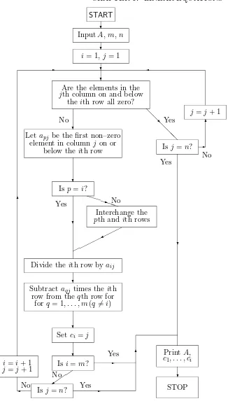
A flow–chart for the Gauss–Jordan algorithm, based on [1, page 83] is pre-sented in figure 1.1 below.
1.4
Systematic solution of linear systems.
Suppose a system ofm linear equations innunknownsx1,· · ·, xn has aug-mented matrix A and that A is row–equivalent to a matrix B which is in reduced row–echelon form, via the Gauss–Jordan algorithm. ThenAandB
arem×(n+ 1). Suppose thatB hasr non–zero rows and that the leading entry 1 in row ioccurs in column numberci, for 1≤i≤r. Then
START
❄ InputA, m, n
❄
i= 1, j= 1 ❄
✲ ✛
❄
Are the elements in the
jth column on and below the ith row all zero?
j=j+ 1 ❅
❅ ❅
❅❅ ❘ Yes No
❄
Is j=n?
Yes No
✲ ✻ Let apj be the first non–zero
element in column j on or below theith row
❄ Is p=i?
Yes
❄
PPPqPPNo
Interchange the
pth and ith rows ✟
✟ ✟ ✟ ✟ ✟ ✟
✙
Divide theith row byaij ❄
Subtractaqj times the ith row from the qth row for
forq = 1, . . . , m(q6=i)
❄ Setci=j
❄ Is i=m?
✑ ✑ ✑ ✰ Is j=n? ✛
i=i+ 1
j=j+ 1 ✻
No No
Yes
Yes✲
✲ ✻
❄
PrintA,
c1, . . . , ci ❄
STOP
Also assume that the remaining column numbers arecr+1,· · ·, cn+1, where 1≤cr+1< cr+2< · · · < cn≤n+ 1.
Case 1: cr = n+ 1. The system is inconsistent. For the last non–zero row ofB is [0,0,· · ·,1] and the corresponding equation is
0x1+ 0x2+· · ·+ 0xn= 1,
which has no solutions. Consequently the original system has no solutions. Case 2: cr ≤n. The system of equations corresponding to the non–zero rows ofB is consistent. First notice thatr≤nhere.
If r=n, thenc1 = 1, c2= 2,· · ·, cn=nand
B =
1 0 · · · 0 d1 0 1 · · · 0 d2
..
. ...
0 0 · · · 1 dn 0 0 · · · 0 0
..
. ...
0 0 · · · 0 0
.
There is a unique solutionx1=d1, x2 =d2,· · ·, xn=dn.
If r < n, there will be more than one solution (infinitely many if the field is infinite). For all solutions are obtained by taking the unknowns
xc1,· · ·, xcr asdependentunknowns and using the r equations
correspond-ing to the non–zero rows of B to express these unknowns in terms of the remaining independent unknowns xcr+1, . . . , xcn, which can take on
arbi-trary values:
xc1 = b1n+1−b1cr+1xcr+1− · · · −b1cnxcn
.. .
xcr = br n+1−brcr+1xcr+1− · · · −brcnxcn.
In particular, taking xcr+1 = 0, . . . , xcn−1 = 0 and xcn = 0,1 respectively,
produces at least two solutions.
EXAMPLE 1.4.1 Solve the system
x+y = 0
Solution. The augmented matrix of the system is
A=
1 1 0 1 −1 1 4 2 1
which is row equivalent to
B =
1 0 12 0 1 −12 0 0 0
.
We read off the unique solution x= 12, y=−12.
(Here n = 2, r = 2, c1 = 1, c2 = 2. Also cr = c2 = 2 < 3 = n+ 1 and
r=n.)
EXAMPLE 1.4.2 Solve the system
2x1+ 2x2−2x3 = 5 7x1+ 7x2+x3 = 10 5x1+ 5x2−x3 = 5.
Solution. The augmented matrix is
A=
2 2 −2 5 7 7 1 10 5 5 −1 5
which is row equivalent to
B =
1 1 0 0 0 0 1 0 0 0 0 1
.
We read off inconsistency for the original system.
(Heren= 3, r= 3, c1= 1, c2= 3. Alsocr=c3 = 4 =n+ 1.)
EXAMPLE 1.4.3 Solve the system
x1−x2+x3 = 1
Solution. The augmented matrix is
A=
·
1 −1 1 1 1 1 −1 2
¸
which is row equivalent to
B =
·
1 0 0 32 0 1 −1 12
¸ .
The complete solution is x1= 32, x2= 12+x3, withx3 arbitrary.
(Here n = 3, r = 2, c1 = 1, c2 = 2. Also cr = c2 = 2 < 4 = n+ 1 and
r < n.)
EXAMPLE 1.4.4 Solve the system
6x3+ 2x4−4x5−8x6 = 8 3x3+x4−2x5−4x6 = 4 2x1−3x2+x3+ 4x4−7x5+x6 = 2 6x1−9x2+ 11x4−19x5+ 3x6 = 1.
Solution. The augmented matrix is
A=
0 0 6 2 −4 −8 8 0 0 3 1 −2 −4 4 2 −3 1 4 −7 1 2 6 −9 0 11 −19 3 1
which is row equivalent to
B =
1 −32 0 116 −196 0 241 0 0 1 13 −2
3 0 53 0 0 0 0 0 1 14 0 0 0 0 0 0 0
.
The complete solution is
x1= 241 + 32x2−116x4+ 196x5,
x3= 53 −13x4+ 23x5,
x6= 14, withx2, x4, x5 arbitrary.
EXAMPLE 1.4.5 Find the rational numbertfor which the following sys-tem is consistent and solve the syssys-tem for this value oft.
x+y = 2
x−y = 0 3x−y = t.
Solution. The augmented matrix of the system is
A=
1 1 2 1 −1 0 3 −1 t
which is row–equivalent to the simpler matrix
B =
1 1 2
0 1 1
0 0 t−2
.
Hence ift 6= 2 the system is inconsistent. If t= 2 the system is consistent and
B=
1 1 2 0 1 1 0 0 0
→
1 0 1 0 1 1 0 0 0
.
We read off the solutionx= 1, y= 1.
EXAMPLE 1.4.6 For which rationals a and b does the following system have (i) no solution, (ii) a unique solution, (iii) infinitely many solutions?
x−2y+ 3z = 4 2x−3y+az = 5 3x−4y+ 5z = b.
Solution. The augmented matrix of the system is
A=
1 −2 3 4 2 −3 a 5 3 −4 5 b
½
R2 →R2−2R1
R3 →R3−3R1
1 −2 3 4
0 1 a−6 −3 0 2 −4 b−12
R3 →R3−2R2
1 −2 3 4
0 1 a−6 −3 0 0 −2a+ 8 b−6
=B.
Case 1. a6= 4. Then −2a+ 86= 0 and we see thatB can be reduced to a matrix of the form
1 0 0 u
0 1 0 v
0 0 1 −b2a+8−6
and we have the unique solutionx=u, y=v, z = (b−6)/(−2a+ 8). Case 2. a= 4. Then
B =
1 −2 3 4 0 1 −2 −3 0 0 0 b−6
.
If b6= 6 we get no solution, whereas ifb= 6 then
B =
1 −2 3 4 0 1 −2 −3
0 0 0 0
R1 → R1 + 2R2
1 0 −1 −2 0 1 −2 −3 0 0 0 0
. We
read off the complete solutionx=−2 +z, y =−3 + 2z, with zarbitrary.
EXAMPLE 1.4.7 Find the reduced row–echelon form of the following ma-trix overZ3:
·
2 1 2 1 2 2 1 0
¸ .
Hence solve the system
2x+y+ 2z = 1 2x+ 2y+z = 0
overZ3.
·
2 1 2 1 2 2 1 0
¸
R2 →R2−R1
·
2 1 2 1 0 1 −1 −1
¸
=
·
2 1 2 1 0 1 2 2
¸
R1 →2R1
·
1 2 1 2 0 1 2 2
¸
R1 →R1+R2
·
1 0 0 1 0 1 2 2
¸
.
The last matrix is in reduced row–echelon form.
To solve the system of equations whose augmented matrix is the given matrix over Z3, we see from the reduced row–echelon form thatx = 1 and
y = 2−2z = 2 +z, where z = 0,1,2. Hence there are three solutions to the given system of linear equations: (x, y, z) = (1, 2,0), (1,0,1) and (1,1,2).
1.5
Homogeneous systems
A system of homogeneous linear equations is a system of the form
a11x1+a12x2+· · ·+a1nxn = 0
a21x1+a22x2+· · ·+a2nxn = 0 .. .
am1x1+am2x2+· · ·+amnxn = 0.
Such a system is always consistent as x1 = 0,· · ·, xn = 0 is a solution. This solution is called the trivial solution. Any other solution is called a non–trivial solution.
For example the homogeneous system
x−y = 0
x+y = 0
has only the trivial solution, whereas the homogeneous system
x−y+z = 0
x+y+z = 0
has the complete solutionx=−z, y = 0, z arbitrary. In particular, taking
z= 1 gives the non–trivial solutionx=−1, y= 0, z= 1.
There is simple but fundamental theorem concerning homogeneous sys-tems.
Proof. Suppose that m < n and that the coefficient matrix of the system is row–equivalent toB, a matrix in reduced row–echelon form. Letr be the number of non–zero rows in B. Then r ≤m < n and hence n−r >0 and so the number n−r of arbitrary unknowns is in fact positive. Taking one of these unknowns to be 1 gives a non–trivial solution.
REMARK 1.5.1 Let two systems of homogeneous equations in n un-knowns have coefficient matrices Aand B, respectively. If each row of B is a linear combination of the rows of A (i.e. a sum of multiples of the rows ofA) and each row ofAis a linear combination of the rows of B, then it is easy to prove that the two systems have identical solutions. The converse is true, but is not easy to prove. Similarly ifA and B have the same reduced row–echelon form, apart from possibly zero rows, then the two systems have identical solutions and conversely.
There is a similar situation in the case of two systems of linear equations (not necessarily homogeneous), with the proviso that in the statement of the converse, the extra condition that both the systems are consistent, is needed.
1.6
PROBLEMS
1. Which of the following matrices of rationals is in reduced row–echelon form?
[Answers:
(a)
·
1 2 0 0 0 0
¸
(b)
·
1 0 −2 0 1 3
¸
(c)
1 0 0 0 1 0 0 0 1
(d)
1 0 0 0 0 0 0 0 0
.]
3. Solve the following systems of linear equations by reducing the augmented matrix to reduced row–echelon form:
(a) x+y+z = 2 (b) x1+x2−x3+ 2x4 = 10 2x+ 3y−z = 8 3x1−x2+ 7x3+ 4x4 = 1
x−y−z = −8 −5x1+ 3x2−15x3−6x4 = 9
(c) 3x−y+ 7z = 0 (d) 2x2+ 3x3−4x4 = 1 2x−y+ 4z = 21 2x3+ 3x4 = 4
x−y+z = 1 2x1+ 2x2−5x3+ 2x4 = 4 6x−4y+ 10z = 3 2x1−6x3+ 9x4 = 7
[Answers: (a) x=−3, y= 194 , z= 14; (b) inconsistent; (c)x=−12 −3z, y =−32−2z, withz arbitrary;
(d)x1 = 192 −9x4, x2=−52 +174x4, x3 = 2−32x4, withx4 arbitrary.] 4. Show that the following system is consistent if and only if c = 2a−3b
and solve the system in this case.
2x−y+ 3z = a
3x+y−5z = b
−5x−5y+ 21z = c.
[Answer: x= a+b5 + 25z, y= −3a+2b5 + 195z, with zarbitrary.]
5. Find the value oftfor which the following system is consistent and solve the system for this value oft.
x+y = 1
tx+y = t
(1 +t)x+ 2y = 3.
6. Solve the homogeneous system
−3x1+x2+x3+x4 = 0
x1−3x2+x3+x4 = 0
x1+x2−3x3+x4 = 0
x1+x2+x3−3x4 = 0.
[Answer: x1 =x2=x3 =x4, withx4 arbitrary.]
7. For which rational numbersλdoes the homogeneous system
x+ (λ−3)y = 0 (λ−3)x+y = 0
have a non–trivial solution? [Answer: λ= 2,4.]
8. Solve the homogeneous system
3x1+x2+x3+x4 = 0 5x1−x2+x3−x4 = 0.
[Answer: x1 =−14x3, x2=−14x3−x4, withx3 and x4 arbitrary.]
9. Let A be the coefficient matrix of the following homogeneous system of
nequations inn unknowns:
(1−n)x1+x2+· · ·+xn = 0
x1+ (1−n)x2+· · ·+xn = 0
· · · = 0
x1+x2+· · ·+ (1−n)xn = 0.
Find the reduced row–echelon form ofAand hence, or otherwise, prove that the solution of the above system is x1 =x2 =· · ·=xn, withxn arbitrary. 10. Let A =
· a b c d
¸
be a matrix over a field F. Prove that A is row–
equivalent to
·
1 0 0 1
¸
11. For which rational numbers a does the following system have (i) no solutions (ii) exactly one solution (iii) infinitely many solutions?
x+ 2y−3z = 4 3x−y+ 5z = 2 4x+y+ (a2−14)z = a+ 2.
[Answer: a = −4, no solution; a = 4, infinitely many solutions; a 6= ±4, exactly one solution.]
12. Solve the following system of homogeneous equations overZ2:
x1+x3+x5 = 0
x2+x4+x5 = 0
x1+x2+x3+x4 = 0
x3+x4 = 0.
[Answer: x1=x2 =x4+x5, x3=x4, with x4 and x5 arbitrary elements of Z2.]
13. Solve the following systems of linear equations overZ5:
(a) 2x+y+ 3z = 4 (b) 2x+y+ 3z = 4 4x+y+ 4z = 1 4x+y+ 4z = 1 3x+y+ 2z = 0 x+y = 3.
[Answer: (a) x = 1, y = 2, z = 0; (b) x = 1 + 2z, y = 2 + 3z, with z an arbitrary element ofZ5.]
14. If (α1, . . . , αn) and (β1, . . . , βn) are solutions of a system of linear equa-tions, prove that
((1−t)α1+tβ1, . . . ,(1−t)αn+tβn) is also a solution.
16. Find the values ofaand b for which the following system is consistent. Also find the complete solution whena=b= 2.
x+y−z+w = 1
ax+y+z+w = b
3x+ 2y+ aw = 1 +a.
[Answer: a6= 2 or a= 2 =b;x= 1−2z, y= 3z−w, withz, w arbitrary.] 17. LetF ={0,1, a, b} be a field consisting of 4 elements.
(a) Determine the addition and multiplication tables ofF. (Hint: Prove that the elements 1 + 0,1 + 1,1 +a,1 +bare distinct and deduce that 1 + 1 + 1 + 1 = 0; then deduce that 1 + 1 = 0.)
(b) A matrix A, whose elements belong toF, is defined by
A=
1 a b a
a b b 1
1 1 1 a
,
prove that the reduced row–echelon form ofA is given by the matrix
B =
1 0 0 0 0 1 0 b
0 0 1 1
MATRICES
2.1
Matrix arithmetic
A matrix over a fieldF is a rectangular array of elements fromF. The sym-bolMm×n(F) denotes the collection of allm×nmatrices overF. Matrices will usually be denoted by capital letters and the equationA= [aij] means that the element in the i–th row and j–th column of the matrix A equals
aij. It is also occasionally convenient to write aij = (A)ij. For the present, all matrices will have rational entries, unless otherwise stated.
EXAMPLE 2.1.1 The formula aij = 1/(i+j) for 1≤ i≤ 3,1 ≤ j ≤4 defines a 3×4 matrix A= [aij], namely
A=
1
2 13 14 15 1
3 1 4
1 5
1 6 1
4 15 16 17
.
DEFINITION 2.1.1 (Equality of matrices) MatricesAandBare said to be equal if A and B have the same size and corresponding elements are equal; that isA and B ∈Mm×n(F) and A= [aij], B = [bij], with aij =bij for 1≤i≤m, 1≤j ≤n.
DEFINITION 2.1.2 (Addition of matrices) Let A = [aij] and B = [bij] be of the same size. Then A+B is the matrix obtained by adding corresponding elements ofA and B; that is
A+B = [aij] + [bij] = [aij+bij].
DEFINITION 2.1.3 (Scalar multiple of a matrix) LetA= [aij] and
t∈F (that istis ascalar). Then tAis the matrix obtained by multiplying all elements ofA byt; that is
tA=t[aij] = [taij].
DEFINITION 2.1.4 (Additive inverse of a matrix) Let A = [aij] . Then −A is the matrix obtained by replacing the elements of A by their additive inverses; that is
−A=−[aij] = [−aij].
DEFINITION 2.1.5 (Subtraction of matrices) Matrix subtraction is defined for two matrices A = [aij] and B = [bij] of the same size, in the usual way; that is
A−B = [aij]−[bij] = [aij−bij].
DEFINITION 2.1.6 (The zero matrix) For each m, n the matrix in
Mm×n(F), all of whose elements are zero, is called the zero matrix (of size
m×n) and is denoted by the symbol 0.
The matrix operations of addition, scalar multiplication, additive inverse and subtraction satisfy the usual laws of arithmetic. (In what follows,sand
twill be arbitrary scalars and A, B, C are matrices of the same size.)
1. (A+B) +C=A+ (B+C);
2. A+B =B+A;
3. 0 +A=A;
4. A+ (−A) = 0;
5. (s+t)A=sA+tA, (s−t)A=sA−tA;
6. t(A+B) =tA+tB, t(A−B) =tA−tB;
7. s(tA) = (st)A;
8. 1A=A, 0A= 0, (−1)A=−A;
9. tA= 0⇒t= 0 or A= 0.
DEFINITION 2.1.7 (Matrix product) Let A = [aij] be a matrix of
Matrix multiplication obeys many of the familiar laws of arithmetic apart from the commutative law.
1. (AB)C=A(BC) if A, B, C arem×n, n×p, p×q, respectively;
2. t(AB) = (tA)B =A(tB), A(−B) = (−A)B =−(AB); 3. (A+B)C=AC+BC ifA and B are m×nand C is n×p;
4. D(A+B) =DA+DB ifAand B arem×n andD isp×m. We prove the associative law only:
Similarly
However the double summations are equal. For sums of the form n
represent the sum of thenpelements of the rectangular array [djk], by rows and by columns, respectively. Consequently
((AB)C)il= (A(BC))il for 1≤i≤m, 1≤l≤q. Hence (AB)C=A(BC).
The system of mlinear equations in nunknowns
a11x1+a12x2+· · ·+a1nxn = b1
a21x1+a22x2+· · ·+a2nxn = b2 .. .
am1x1+am2x2+· · ·+amnxn = bm is equivalent to a single matrix equation
is the vector of unknowns and B =
is the vector of
constants.
EXAMPLE 2.1.3 The system
x+y+z = 1
x−y+z = 0.
is equivalent to the matrix equation
·
1 1 1 1 −1 1
¸
x y z
= ·
1 0
¸
and to the equation
x ·
1 1
¸
+y ·
1
−1
¸
+z ·
1 1
¸
=
·
1 0
¸ .
2.2
Linear transformations
An n–dimensional column vectoris an n×1 matrix overF. The collection of alln–dimensional column vectors is denoted by Fn.
Every matrix is associated with an important type of function called a linear transformation.
DEFINITION 2.2.1 (Linear transformation) WithA∈Mm×n(F), we associate the function TA : Fn → Fm defined by TA(X) = AX for all
X ∈Fn. More explicitly, using components, the above function takes the form
y1 = a11x1+a12x2+· · ·+a1nxn
y2 = a21x1+a22x2+· · ·+a2nxn ..
.
ym = am1x1+am2x2+· · ·+amnxn,
wherey1, y2,· · ·, ym are the components of the column vector TA(X). The function just defined has the property that
TA(sX+tY) =sTA(X) +tTA(Y) (2.1) for alls, t∈F and all n–dimensional column vectorsX, Y. For
REMARK 2.2.1 It is easy to prove that if T : Fn → Fm is a function satisfying equation 2.1, thenT =TA, where A is the m×n matrix whose columns are T(E1), . . . , T(En), respectively, where E1, . . . , En are the n– dimensionalunit vectors defined by
E1 =
1 0 .. . 0
, . . . , En=
0 0 .. . 1
.
One well–known example of a linear transformation arises from rotating the (x, y)–plane in 2-dimensional Euclidean space, anticlockwise through θ
radians. Here a point (x, y) will be transformed into the point (x1, y1), where
x1 = xcosθ−ysinθ
y1 = xsinθ+ycosθ.
In 3–dimensional Euclidean space, the equations
x1 =xcosθ−ysinθ, y1 =xsinθ+ycosθ, z1 =z;
x1 =x, y1 =ycosφ−zsinφ, z1=ysinφ+zcosφ;
x1 =xcosψ−zsinψ, y1=y, z1=xsinψ+zcosψ;
correspond to rotations about the positivez, x, y–axes, anticlockwise through
θ, φ, ψradians, respectively.
The product of two matrices is related to the product of the correspond-ing linear transformations:
IfAism×nandBisn×p, then the functionTATB :Fp→Fm, obtained by first performingTB, thenTAis in fact equal to the linear transformation
TAB. For ifX∈Fp, we have
TATB(X) =A(BX) = (AB)X=TAB(X).
The following example is useful for producing rotations in 3–dimensional animated design. (See [27, pages 97–112].)
θ
l
(x1, y1)
¡¡ ¡¡
¡¡ ¡¡
¡ ¡ ¡ ¡ ¡
❅ ❅ ❅ ❅
❅ ❅
❅
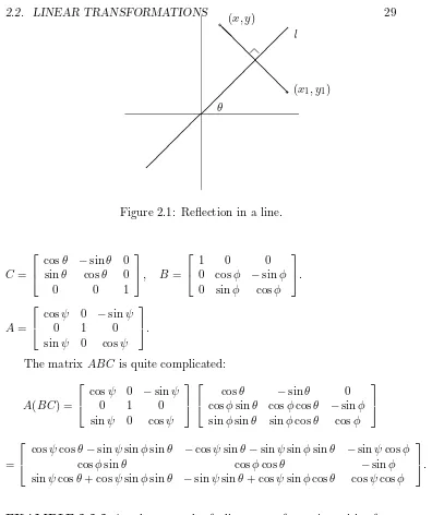
Figure 2.1: Reflection in a line.
C=
cosθ −sinθ 0 sinθ cosθ 0
0 0 1
, B =
1 0 0
0 cosφ −sinφ
0 sinφ cosφ
.
A=
cosψ 0 −sinψ
0 1 0
sinψ 0 cosψ
.
The matrix ABC is quite complicated:
A(BC) =
cosψ 0 −sinψ
0 1 0
sinψ 0 cosψ
cosθ −sinθ 0 cosφsinθ cosφcosθ −sinφ
sinφsinθ sinφcosθ cosφ
=
cosψcosθ−sinψsinφsinθ −cosψsinθ−sinψsinφsinθ −sinψcosφ
cosφsinθ cosφcosθ −sinφ
sinψcosθ+ cosψsinφsinθ −sinψsinθ+ cosψsinφcosθ cosψcosφ
.
EXAMPLE 2.2.2 Another example of a linear transformation arising from geometry is reflection of the plane in a line l inclined at an angle θ to the positivex–axis.
θ
Figure 2.2: Projection on a line.
In terms of matrices, we get transformation equations
·
The more general transformation
·
represents a rotation, followed by a scaling and then by a translation. Such transformations are important in computer graphics. See [23, 24].
EXAMPLE 2.2.3 Our last example of a geometrical linear transformation arises from projecting the plane onto a line l through the origin, inclined at angle θ to the positive x–axis. Again we reduce that problem to the simpler case where l is the x–axis and the equations of transformation are
x1 =x, y1 = 0.
In terms of matrices, we get transformation equations
=
·
cosθ 0 sinθ 0
¸ ·
cosθ sinθ
−sinθ cosθ ¸ ·
x y
¸
=
·
cos2θ cosθsinθ sinθcosθ sin2θ
¸ · x y
¸ .
2.3
Recurrence relations
DEFINITION 2.3.1 (The identity matrix) The n ×n matrix In = [δij], defined by δij = 1 ifi=j, δij = 0 if i6=j, is called the n×n identity matrix of order n. In other words, the columns of the identity matrix of order nare the unit vectorsE1,· · ·, En, respectively.
For example, I2 =
·
1 0 0 1
¸
.
THEOREM 2.3.1 If A ism×n, thenImA=A=AIn.
DEFINITION 2.3.2 (k–th power of a matrix) IfAis ann×nmatrix, we defineAk recursively as follows: A0=I
n andAk+1=AkA fork≥0. For exampleA1 =A0A=InA=Aand henceA2 =A1A=AA.
The usual index laws hold providedAB=BA:
1. AmAn=Am+n, (Am)n=Amn; 2. (AB)n=AnBn;
3. AmBn=BnAm;
4. (A+B)2 =A2+ 2AB+B2;
5. (A+B)n= n
X
i=0
¡n
i
¢
AiBn−i;
6. (A+B)(A−B) =A2−B2.
We now state a basic property of the natural numbers.
AXIOM 2.3.1 (PRINCIPLE OF MATHEMATICAL INDUCTION)
(ii) the truth of Pn implies that ofPn+1 for each n≥1, thenPn is true for alln≥1.
EXAMPLE 2.3.1 LetA=
·
7 4
−9 −5
¸
.Prove that
An=
·
1 + 6n 4n
−9n 1−6n ¸
if n≥1.
Solution. We use the principle of mathematical induction.
Take Pn to be the statement
An=
·
1 + 6n 4n
−9n 1−6n ¸
.
ThenP1 asserts that
A1 =
·
1 + 6×1 4×1
−9×1 1−6×1
¸
=
·
7 4
−9 −5
¸ ,
which is true. Now letn≥1 and assume thatPnis true. We have to deduce that
An+1=
·
1 + 6(n+ 1) 4(n+ 1)
−9(n+ 1) 1−6(n+ 1)
¸
=
·
7 + 6n 4n+ 4
−9n−9 −5−6n ¸
.
Now
An+1 = AnA
=
·
1 + 6n 4n
−9n 1−6n ¸ ·
7 4
−9 −5
¸
=
·
(1 + 6n)7 + (4n)(−9) (1 + 6n)4 + (4n)(−5) (−9n)7 + (1−6n)(−9) (−9n)4 + (1−6n)(−5)
¸
=
·
7 + 6n 4n+ 4
−9n−9 −5−6n ¸
,
and “the induction goes through”.
EXAMPLE 2.3.2 The following system of recurrence relations holds for alln≥0:
xn+1 = 7xn+ 4yn
yn+1 = −9xn−5yn. Solve the system forxn and yn in terms ofx0 and y0.
Solution. Combine the above equations into a single matrix equation
· xn+1
yn+1
¸
=
·
7 4
−9 −5
¸ · xn
yn
¸ ,
orXn+1 =AXn, whereA=
·
7 4
−9 −5
¸
and Xn=
· xn
yn
¸
. We see that
X1 = AX0
X2 = AX1=A(AX0) =A2X0 ..
.
Xn = AnX0.
(The truth of the equation Xn = AnX0 for n ≥ 1, strictly speaking follows by mathematical induction; however for simple cases such as the above, it is customary to omit the strict proof and supply instead a few lines of motivation for the inductive statement.)
Hence the previous example gives
· xn
yn
¸
=Xn =
·
1 + 6n 4n
−9n 1−6n ¸ ·
x0
y0
¸
=
·
(1 + 6n)x0+ (4n)y0 (−9n)x0+ (1−6n)y0
¸ ,
and hencexn= (1 + 6n)x0+ 4ny0andyn= (−9n)x0+ (1−6n)y0, forn≥1.
2.4
PROBLEMS
1. LetA, B, C, D be matrices defined by
A=
3 0
−1 2 1 1
, B =
1 5 2
−1 1 0
−4 1 3
C=
Which of the following matrices are defined? Compute those matrices which are defined.
A+B, A+C, AB, BA, CD, DC, D2.
for suitable numbers a and b. Use the associative law to show that (BA)2B =B. induction, to prove that
whereA =
· a b
1 0
¸
and hence express
· xn+1
xn
¸
in terms of
· x1
x0
¸
. If a= 4 and b =−3, use the previous question to find a formula for
xn in terms ofx1 and x0. [Answer:
xn=
3n−1 2 x1+
3−3n 2 x0.]
6. LetA=
·
2a −a2
1 0
¸
.
(a) Prove that
An=
·
(n+ 1)an −nan+1 nan−1 (1−n)an
¸
ifn≥1.
(b) A sequencex0, x1, . . . , xn, . . .satisfies the recurrence relationxn+1 = 2axn−a2xn−1 forn≥1. Use part (a) and the previous question to prove thatxn=nan−1x1+ (1−n)anx0 forn≥1.
7. Let A =
· a b
c d ¸
and suppose that λ1 and λ2 are the roots of the quadratic polynomialx2−(a+d)x+ad−bc. (λ
1andλ2 may be equal.) Letknbe defined by k0 = 0, k1 = 1 and forn≥2
kn= n
X
i=1
λn1−iλi2−1.
Prove that
kn+1= (λ1+λ2)kn−λ1λ2kn−1, ifn≥1. Also prove that
kn=
½
(λn1 −λn2)/(λ1−λ2) ifλ16=λ2,
nλn1−1 ifλ1=λ2. Use mathematical induction to prove that ifn≥1,
An=knA−λ1λ2kn−1I2, [Hint: Use the equationA2= (a+d)A−(ad−bc)I
8. Use Question 6 to prove that ifA=
·
1 2 2 1
¸
, then
An= 3 n 2
·
1 1 1 1
¸
+(−1) n−1 2
·
−1 1 1 −1
¸
ifn≥1.
9. The Fibonacci numbers are defined by the equations F0 = 0, F1 = 1 andFn+1=Fn+Fn−1 ifn≥1. Prove that
Fn= √1 5
ÃÃ
1 +√5 2
!n
−
Ã
1−√5 2
!n!
ifn≥0.
10. Let r > 1 be an integer. Let a and b be arbitrary positive integers. Sequencesxnand ynof positive integers are defined in terms ofaand
bby the recurrence relations
xn+1 = xn+ryn
yn+1 = xn+yn, forn≥0, where x0 =aand y0 =b.
Use Question 6 to prove that
xn
yn →
√
r asn→ ∞.
2.5
Non–singular matrices
DEFINITION 2.5.1 (Non–singular matrix)
A square matrix A ∈ Mn×n(F) is called non–singular or invertible if there exists a matrix B∈Mn×n(F) such that
AB=In=BA.
THEOREM 2.5.1 (Inverses are unique)
If Ahas inverses B andC, then B=C.
Proof. Let B and C be inverses of A. Then AB = In = BA and AC =
In=CA. ThenB(AC) =BIn=B and (BA)C=InC=C. Hence because
B(AC) = (BA)C, we deduce thatB=C.
REMARK 2.5.1 If Ahas an inverse, it is denoted by A−1. So
AA−1=In=A−1A.
Also if Ais non–singular, it follows that A−1 is also non–singular and (A−1)−1=A.
THEOREM 2.5.2 IfAand B are non–singular matrices of the same size, then so is AB. Moreover
(AB)−1 =B−1A−1. Proof.
(AB)(B−1A−1) =A(BB−1)A−1 =AInA−1 =AA−1=In. Similarly
(B−1A−1)(AB) =In.
REMARK 2.5.2 The above result generalizes to a product of m non– singular matrices: IfA1, . . . , Am are non–singularn×n matrices, then the productA1. . . Am is also non–singular. Moreover
(A1. . . Am)−1 =A−m1. . . A−11.
(Thus the inverse of the product equals the product of the inverses in the reverse order.)
EXAMPLE 2.5.1 If A and B are n×n matrices satisfying A2 = B2 = (AB)2 =In, prove thatAB=BA.
Solution. Assume A2 = B2 = (AB)2 = In. Then A, B, AB are non– singular andA−1=A, B−1 =B,(AB)−1 =AB.
EXAMPLE 2.5.2 A =
·
1 2 4 8
¸
is singular. For suppose B =
·
and equating the corresponding elements of column 1 of both sides gives the system
a+ 2c = 1 4a+ 8c = 0
which is clearly inconsistent.
THEOREM 2.5.3 Let A =
REMARK 2.5.3 The expression ad−bc is called the determinant of A
and is denoted by the symbols detA or
¯
satisfies the equation
AB=I2 =BA.
EXAMPLE 2.5.3 Let
A= Solution. After verifying thatA3 = 5I
THEOREM 2.5.4 If the coefficient matrix A of a system of n equations in n unknowns is non–singular, then the system AX = B has the unique solution X=A−1B.
Proof. Assume that A−1 exists.
1. (Uniqueness.) Assume thatAX =B. Then
(A−1A)X = A−1B, InX = A−1B,
X = A−1B.
2. (Existence.) LetX =A−1B. Then
AX = A(A−1B) = (AA−1)B =InB =B.
THEOREM 2.5.5 (Cramer’s rule for 2 equations in 2 unknowns)
The system
ax+by = e cx+dy = f
has a unique solution if ∆ =
¯ ¯ ¯ ¯
a b c d
¯ ¯ ¯ ¯6
= 0, namely
x= ∆1
∆, y= ∆2
∆, where
∆1=
¯ ¯ ¯ ¯
e b f d
¯ ¯ ¯ ¯
and ∆2 =
¯ ¯ ¯ ¯
a e c f
¯ ¯ ¯ ¯ .
Proof. Suppose ∆6= 0. Then A=
· a b c d
¸
has inverse
A−1 = ∆−1
·
d −b
−c a ¸
and we know that the system
A ·
x y
¸
=
· e f
has the unique solution
COROLLARY 2.5.1 The homogeneous system
ax+by = 0
cx+dy = 0
has only the trivial solution if ∆ =
¯
EXAMPLE 2.5.4 The system
7x+ 8y = 100
THEOREM 2.5.6 Let A be a square matrix. If A is non–singular, the homogeneous system AX = 0 has only the trivial solution. Equivalently, if the homogenous system AX = 0 has a non–trivial solution, then A is singular. not all zero, such that
that is, if the columns of A are linearly dependent, then A is singular. An equivalent way of saying that the columns ofAare linearly dependent is that one of the columns of A is expressible as a sum of certain scalar multiples of the remaining columns of A; that is one column is a linear combination of the remaining columns.
EXAMPLE 2.5.5
A=
1 2 3 1 0 1 3 4 7
is singular. For it can be verified thatA has reduced row–echelon form
1 0 1 0 1 1 0 0 0
and consequentlyAX = 0 has a non–trivial solutionx=−1, y=−1, z= 1.
REMARK 2.5.5 More generally, if A is row–equivalent to a matrix con-taining a zero row, then A is singular. For then the homogeneous system
AX= 0 has a non–trivial solution.
An important class of non–singular matrices is that of the elementary row matrices.
DEFINITION 2.5.2 (Elementary row matrices) There are three types,
Eij, Ei(t), Eij(t), corresponding to the three kinds of elementary row oper-ation:
1. Eij,(i6=j) is obtained from the identity matrixIn by interchanging rowsi andj.
2. Ei(t),(t6= 0) is obtained by multiplying thei–th row ofIn by t. 3. Eij(t),(i=6 j) is obtained from In by adding ttimes the j–th row of
In to thei–th row. EXAMPLE 2.5.6 (n= 3.)
E23=
1 0 0 0 0 1 0 1 0
, E2(−1) =
1 0 0 0 −1 0 0 0 1
, E23(−1) =
1 0 0 0 1 −1 0 0 1
The elementary row matrices have the following distinguishing property:
THEOREM 2.5.7 If a matrix Ais pre–multiplied by an elementary row– matrix, the resulting matrix is the one obtained by performing the corre-sponding elementary row–operation onA.
EXAMPLE 2.5.7
E23
a b c d e f
=
1 0 0 0 0 1 0 1 0
a b c d e f
=
a b e f c d
.
COROLLARY 2.5.2 The three types of elementary row–matrices are non– singular. Indeed
1. Eij−1=Eij; 2. Ei−1(t) =Ei(t−1); 3. (Eij(t))−1 =Eij(−t).
Proof. Taking A = In in the above theorem, we deduce the following equations:
EijEij = In
Ei(t)Ei(t−1) = In=Ei(t−1)Ei(t) ift6= 0
Eij(t)Eij(−t) = In=Eij(−t)Eij(t).
EXAMPLE 2.5.8 Find the 3×3 matrix A = E3(5)E23(2)E12 explicitly. Also findA−1.
Solution.
A=E3(5)E23(2)
0 1 0 1 0 0 0 0 1
=E3(5)
0 1 0 1 0 2 0 0 1
=
0 1 0 1 0 2 0 0 5
.
To find A−1, we have
= E12E23(−2)
1 0 0 0 1 0 0 0 15
= E12
1 0 0 0 1 −2 5 0 0 15
=
0 1 −25 1 0 0 0 0 15
.
REMARK 2.5.6 Recall thatAandB are row–equivalent ifB is obtained from A by a sequence of elementary row operations. If E1, . . . , Er are the respective corresponding elementary row matrices, then
B =Er(. . .(E2(E1A)). . .) = (Er. . . E1)A=P A,
where P = Er. . . E1 is non–singular. Conversely if B = P A, where P is non–singular, thenA is row–equivalent to B. For as we shall now see, P is in fact a product of elementary row matrices.
THEOREM 2.5.8 Let Abe non–singular n×nmatrix. Then
(i) Ais row–equivalent to In,
(ii) Ais a product of elementary row matrices.
Proof. Assume thatAis non–singular and letBbe the reduced row–echelon form of A. Then B has no zero rows, for otherwise the equation AX = 0 would have a non–trivial solution. ConsequentlyB =In.
It follows that there exist elementary row matricesE1, . . . , Er such that
Er(. . .(E1A). . .) = B = In and hence A = E1−1. . . Er−1, a product of elementary row matrices.
THEOREM 2.5.9 Let A ben×nand suppose thatA is row–equivalent to In. Then A is non–singular and A−1 can be found by performing the same sequence of elementary row operations on In as were used to convert
AtoIn.
Proof. Suppose that Er. . . E1A = In. In other words BA = In, where
B = Er. . . E1 is non–singular. Then B−1(BA) =B−1In and so A =B−1, which is non–singular.
Also A−1 =¡
B−1¢−1
REMARK 2.5.7 It follows from theorem 2.5.9 that ifA is singular, then
Ais row–equivalent to a matrix whose last row is zero.
EXAMPLE 2.5.9 Show thatA=
·
1 2 1 1
¸
is non–singular, findA−1 and expressAas a product of elementary row matrices.
Solution. We form thepartitionedmatrix [A|I2] which consists ofAfollowed byI2. Then any sequence of elementary row operations which reducesA to
I2 will reduce I2 toA−1. Here [A|I2] =
·
1 2 1 0 1 1 0 1
¸
R2 →R2−R1
·
1 2 1 0
0 −1 −1 1
¸
R2 →(−1)R2
·
1 2 1 0 0 1 1 −1
¸
R1 →R1−2R2
·
1 0 −1 2 0 1 1 −1
¸ .
Hence Ais row–equivalent to I2 andA is non–singular. Also
A−1 =
·
−1 2 1 −1
¸ .
We also observe that
E12(−2)E2(−1)E21(−1)A=I2.
Hence
A−1 = E12(−2)E2(−1)E21(−1)
A = E21(1)E2(−1)E12(2).
The next result is the converse of Theorem 2.5.6 and is useful for proving the non–singularity of certain types of matrices.
THEOREM 2.5.10 Let A be an n×n matrix with the property that the homogeneous system AX = 0 has only the trivial solution. Then A is non–singular. Equivalently, if A is singular, then the homogeneous system
Proof. If A is n×n and the homogeneous system AX = 0 has only the trivial solution, then it follows that the reduced row–echelon form B of A
cannot have zero rows and must therefore be In. HenceA is non–singular. COROLLARY 2.5.3 Suppose that A and B are n×n and AB = In. ThenBA=In.
Proof. Let AB = In, where A and B are n×n. We first show that B is non–singular. Assume BX = 0. Then A(BX) = A0 = 0, so (AB)X = 0, InX= 0 and henceX= 0.
Then from AB=In we deduce (AB)B−1=InB−1 and henceA=B−1. The equationBB−1=I
n then givesBA=In.
Before we give the next example of the above criterion for non-singularity, we introduce an important matrix operation.
DEFINITION 2.5.3 (The transpose of a matrix) LetAbe anm×n
matrix. ThenAt, thetransposeofA, is the matrix obtained by interchanging the rows and columns of A. In other words if A = [aij], then ¡At¢ji =aij. ConsequentlyAt is n×m.
The transpose operation has the following properties:
1. ¡ At¢t
=A;
2. (A±B)t=At±Bt ifAand B arem×n; 3. (sA)t=sAt ifsis a scalar;
4. (AB)t=BtAt ifAis m×nand B isn×p;
5. IfA is non–singular, thenAt is also non–singular and
¡ At¢−1
=¡ A−1¢t
;
6. XtX=x21+. . .+x2n ifX = [x1, . . . , xn]tis a column vector.
We prove only the fourth property. First check that both (AB)t and BtAt have the same size (p ×m). Moreover, corresponding elements of both matrices are equal. For ifA= [aij] and B= [bjk], we have
¡
(AB)t¢
ki = (AB)ik =
n
X
j=1
= n
X
j=1
¡ Bt¢
kj
¡ At¢
ji = ¡
BtAt¢
ki.
There are two important classes of matrices that can be defined concisely in terms of the transpose operation.
DEFINITION 2.5.4 (Symmetric matrix) A real matrixAis called sym-metricif At =A. In other words A is square (n×n say) and a
ji =aij for all 1≤i≤n, 1≤j≤n. Hence
A=
· a b
b c ¸
is a general 2×2 symmetric matrix.
DEFINITION 2.5.5 (Skew–symmetric matrix) A real matrixAis called skew–symmetric if At = −A. In other words A is square (n×n say) and
aji =−aij for all 1≤i≤n, 1≤j≤n.
REMARK 2.5.8 Takingi=j in the definition of skew–symmetric matrix givesaii=−aii and so aii= 0. Hence
A=
·
0 b
−b 0
¸
is a general 2×2 skew–symmetric matrix.
We can now state a second application of the above criterion for non– singularity.
COROLLARY 2.5.4 Let B be an n×n skew–symmetric matrix. Then
A=In−B is non–singular.
Proof. Let A=In−B, where Bt=−B. By Theorem 2.5.10 it suffices to show that AX= 0 implies X= 0.
We have (In−B)X= 0, so X=BX. Hence XtX=XtBX. Taking transposes of both sides gives
(XtBX)t = (XtX)t
XtBt(Xt)t = Xt(Xt)t
Xt(−B)X = XtX
−XtBX = XtX =XtBX.
HenceXtX=−XtX and XtX= 0. But if X= [x1, . . . , xn]t, thenXtX =
x2
2.6
Least squares solution of equations
Suppose AX = B represents a system of linear equations with real coeffi-cients which may be inconsistent, because of the possibility of experimental errors in determiningA orB. For example, the system
x = 1
y = 2
x+y = 3.001
is inconsistent.
It can be proved that the associated system AtAX = AtB is always consistent and that any solution of this system minimizes the sumr12+. . .+
rm2, wherer1, . . . , rm (the residuals) are defined by
ri =ai1x1+. . .+ainxn−bi,
fori= 1, . . . , m. The equations represented by AtAX=AtB are called the normal equations corresponding to the system AX = B and any solution of the system of normal equations is called a least squares solution of the original system.
EXAMPLE 2.6.1 Find a least squares solution of the above inconsistent system.
Solution. HereA=
1 0 0 1 1 1
, X= ·
x y
¸ , B =
1 2 3.001
.
ThenAtA=
·
1 0 1 0 1 1
¸
1 0 0 1 1 1
= ·
2 1 1 2
¸
.
Also AtB =
·
1 0 1 0 1 1
¸
1 2 3.001
= ·
4.001 5.001
¸
.
So the normal equations are
2x+y = 4.001
x+ 2y = 5.001
which have the unique solution
x= 3.001
3 , y= 6.001
EXAMPLE 2.6.2 Points (x1, y1), . . . ,(xn, yn) are experimentally deter-mined and should lie on a liney=mx+c. Find a least squares solution to the problem.
Solution. The points have to satisfy
mx1+c = y1
It is not difficult to prove that
∆ = det (AtA) = X 1≤i<j≤n
(xi−xj)2,
which is positive unless x1 = . . . = xn. Hence if not all of x1, . . . , xn are equal,AtAis non–singular and the normal equations have a unique solution. This can be shown to be
m= 1
2.7
PROBLEMS
1. Let A =
·
1 4
−3 1
¸
. Prove that A is non–singular, find A−1 and expressAas a product of elementary row matrices.
[Answer: A−1 =
· 1
13 −134 3 13 131
¸
,
A=E21(−3)E2(13)E12(4) is one such decomposition.]
2. A square matrixD= [dij] is calleddiagonalifdij = 0 fori6=j. (That is the off–diagonal elements are zero.) Prove that pre–multiplication of a matrix A by a diagonal matrix D results in matrix DA whose rows are the rows ofA multiplied by the respective diagonal elements of D. State and prove a similar result for post–multiplication by a diagonal matrix.
Let diag (a1, . . . , an) denote the diagonal matrix whose diagonal ele-mentsdii area1, . . . , an, respectively. Show that
diag (a1, . . . , an)diag (b1, . . . , bn) = diag (a1b1, . . . , anbn)
and deduce that ifa1. . . an6= 0, then diag (a1, . . . , an) is non–singular and
(diag (a1, . . . , an))−1= diag (a−11, . . . , a−n1).
Also prove that diag (a1, . . . , an) is singular if ai = 0 for some i.
3. Let A =
0 0 2 1 2 6 3 7 9
. Prove that A is non–singular, find A−1 and
expressAas a product of elementary row matrices.
[Answers: A−1 =
−12 7 −2 9
2 −3 1 1
2 0 0
,
4. Find the rational numberkfor which the matrixA=
1 2 k
3 −1 1 5 3 −5
is singular. [Answer: k=−3.]
5. Prove thatA=
·
1 2
−2 −4
¸
is singular and find a non–singular matrix
P such thatP A has last row zero.
6. If A =
·
1 4
−3 1
¸
, verify that A2 −2A+ 13I
2 = 0 and deduce that
A−1=−1
13(A−2I2).
7. LetA=
1 1 −1 0 0 1 2 1 2
.
(i) Verify thatA3= 3A2−3A+I3. (ii) Express A4 in terms of A2, A and I
3 and hence calculate A4 explicitly.
(iii) Use (i) to prove thatA is non–singular and findA−1 explicitly.
[Answers: (ii) A4 = 6A2−8A+ 3I3 =
−11 −8 −4 12 9 4 20 16 5
;
(iii)A−1=A2−3A+ 3I3=
−1 −3 1 2 4 −1
0 1 0
.]
8. (i) LetB be ann×nmatrix such thatB3 = 0. IfA=In−B, prove thatA is non–singular andA−1=In+B+B2.
Show that the system of linear equationsAX =bhas the solution
X =b+Bb+B2b.
(ii) IfB =
0 r s
0 0 t
0 0 0
, verify thatB3= 0 and use (i) to determine
[Answer: 10. Use Question 7 to solve the system of equations
x+y−z = a
z = b
2x+y+ 2z = c
wherea, b, care given rationals. Check your answer using the Gauss– Jordan algorithm.
[Answer: x=−a−3b+c, y = 2a+ 4b−c, z=b.]
11. Determine explicitly the following products of 3×3 elementary row matrices.
12. LetA be the following product of 4×4 elementary row matrices:
13. Determine which of the following matrices over Z2 are non–singular and find the inverse, where possible.
(a)
14. Determine which of the following matrices are non–singular and find the inverse, where possible.
(a)
17. Prove that the real matrix A =
is non–singular by
proving thatA is row–equivalent toI3.
18. IfP−1AP =B, prove thatP−1AnP =Bn forn≥1.
and deduce that
An= 1
be aMarkovmatrix; that is a matrix whose elements
are non–negative and satisfya+c= 1 =b+d. Also letP =
22. Prove that the system of linear equations
x+ 2y = 4
x+y = 5
3x+ 5y = 12
23. The points (0,0),(1,0),(2,−1),(3,4),(4,8) are required to lie on a parabola y = a+bx+cx2. Find a least squares solution for a, b, c. Also prove that no parabola passes through these points.
[Answer: a= 15, b=−2, c= 1.]
24. IfAis a symmetricn×nreal matrix andB isn×m, prove thatBtAB is a symmetricm×mmatrix.
25. IfA ism×n and B is n×m, prove thatAB is singular if m > n.
SUBSPACES
3.1
Introduction
Throughout this chapter, we will be studyingFn, the set of alln–dimensional column vectors with components from a field F. We continue our study of matrices by considering an important class of subsets ofFncalledsubspaces. These arise naturally for example, when we solve a system ofm linear ho-mogeneous equations innunknowns.
We also study the concept of linear dependence of a family of vectors. This was introduced briefly in Chapter 2, Remark 2.5.4. Other topics dis-cussed are the row space, column space and null space of a matrix over F, thedimensionof a subspace, particular examples of the latter being therank and nullityof a matrix.
3.2
Subspaces of
F
nDEFINITION 3.2.1 A subsetS ofFn is called a subspace of Fnif 1. The zero vector belongs to S; (that is, 0∈S);
2. If u ∈ S and v ∈ S, then u+v ∈ S; (S is said to be closed under vector addition);
3. Ifu ∈S and t∈F, then tu ∈S; (S is said to be closed under scalar multiplication).
EXAMPLE 3.2.1 Let A ∈ Mm×n(F). Then the set of vectors X ∈ Fn satisfying AX = 0 is a subspace of Fn called the null space of A and is denoted here by N(A). (It is sometimes called the solution spaceofA.)
Proof. (1) A0 = 0, so 0 ∈ N(A); (2) If X, Y ∈ N(A), then AX = 0 and
AY = 0, soA(X+Y) =AX+AY = 0 + 0 = 0 and soX+Y ∈N(A); (3) IfX∈N(A) and t∈F, thenA(tX) =t(AX) =t0 = 0, sotX ∈N(A).
For example, if A =
·
1 0 0 1
¸
, then N(A) = {0}, the set consisting of
just the zero vector. If A =
·
1 2 2 4
¸
, then N(A) is the set of all scalar multiples of [−2,1]t.
EXAMPLE 3.2.2 Let X1, . . . , Xm ∈ Fn. Then the set consisting of all linear combinations x1X1 +· · ·+xmXm, where x1, . . . , xm ∈ F, is a sub-space of Fn. This subspace is called the subspace spanned or generatedby
X1, . . . , Xm and is denoted here byhX1, . . . , Xmi. We also callX1, . . . , Xm a spanning family forS =hX1, . . . , Xmi.
Proof. (1) 0 = 0X1 +· · ·+ 0Xm, so 0 ∈ hX1, . . . , Xmi; (2) If X, Y ∈
hX1, . . . , Xmi, thenX =x1X1+· · ·+xmXm andY =y1X1+· · ·+ymXm, so
X+Y = (x1X1+· · ·+xmXm) + (y1X1+· · ·+ymXm) = (x1+y1)X1+· · ·+ (xm+ym)Xm∈ hX1, . . . , Xmi. (3) IfX ∈ hX1, . . . , Xmi and t∈F, then
X = x1X1+· · ·+xmXm
tX = t(x1X1+· · ·+xmXm)
= (tx1)X1+· · ·+ (txm)Xm∈ hX1, . . . , Xmi.
For example, ifA∈Mm×n(F), the subspace generated by the columns ofA is an important subspace of Fm and is called the column space of A. The column space of A is denoted here by C(A). Also the subspace generated by the rows ofAis a subspace ofFnand is called the row spaceof Aand is denoted byR(A).
EXAMPLE 3.2.3 For example Fn =hE1, . . . , Eni, where E1, . . . , En are the n–dimensional unit vectors. For if X = [x1, . . . , xn]t ∈ Fn, then X =
x1E1+· · ·+xnEn.
Solution. (S is in fact the null space of [2,−3,5], soS is indeed a subspace ofR3.)
If [x, y, z]t∈S, thenx= 3
2y−52z. Then
x y z
=
3 2y−52z
y z
=y
3 2 1 0
+z
−5 2 0 1
and conversely. Hence [32,1,0]t and [−52,0,1]t form a spanning family for
S.
The following result is easy to prove:
LEMMA 3.2.1 Suppose each of X1, . . . , Xr is a linear combination of
Y1, . . . , Ys. Then any linear combination of X1, . . . , Xr is a linear combi-nation ofY1, . . . , Ys.
As a corollary we have
THEOREM 3.2.1 Subspaces hX1, . . . , Xri and hY1, . . . , Ysi are equal if each ofX1, . . . , Xris a linear combination ofY1, . . . , Ysand each ofY1, . . . , Ys is a linear combination ofX1, . . . , Xr.
COROLLARY 3.2.1 SubspaceshX1, . . . , Xr, Z1, . . . , ZtiandhX1, . . . , Xri are equal if each of Z1, . . . , Ztis a linear combination of X1, . . . , Xr.
EXAMPLE 3.2.5 IfX andY are vectors in Rn, then
hX, Yi=hX+Y, X−Yi.
Solution. Each of X+Y and X−Y is a linear combination of X and Y. Also
X = 1
2(X+Y) + 1
2(X−Y) and Y = 1
2(X+Y)− 1
2(X−Y), so each ofX andY is a linear combination ofX+Y andX−Y.
There is an important application of Theorem 3.2.1 to row equivalent matrices (see Definition 1.2.4):