Basic Hypergeometric Functions
as Limits of Elliptic Hypergeometric Functions
⋆Fokko J. VAN DE BULT and Eric M. RAINS
MC 253-37, California Institute of Technology, 91125, Pasadena, CA, USA E-mail: [email protected], [email protected]
Received February 01, 2009; Published online June 10, 2009 doi:10.3842/SIGMA.2009.059
Abstract. We describe a uniform way of obtaining basic hypergeometric functions as limits of the elliptic beta integral. This description gives rise to the construction of a polytope with a different basic hypergeometric function attached to each face of this polytope. We can subsequently obtain various relations, such as transformations and three-term relations, of these functions by considering geometrical properties of this polytope. The most ge-neral functions we describe in this way are sums of two very-well-poised 10φ9’s and their
Nassrallah–Rahman type integral representation.
Key words: elliptic hypergeometric functions, basic hypergeometric functions, transforma-tion formulas
2000 Mathematics Subject Classification: 33D15
1
Introduction
Hypergeometric functions have played an important role in mathematics, and have been much studied since the time of Euler and Gauß. One of the goals of this research has been to obtain hypergeometric identities, such as evaluation and transformation formulas. Such formulas are of interest due to representation-theoretical interpretations, as well as their use in simplifying sums appearing in combinatorics.
In more recent times people have been trying to understand the structure behind these formu-las. In particular people have studied the symmetry groups associated to certain hypergeometric functions, or the three terms relations satisfied by them (see [8] and [9]).
Another recent development is the advent of elliptic hypergeometric functions. This defines a whole new class of hypergeometric functions, in addition to the ordinary hypergeometric functions and the basic hypergeometric functions. A nice recent overview of this theory is given in [18]. For several of the most important kinds of formulas for classical hypergeometric functions there exist elliptic hypergeometric analogues. It is well known that one obtains basic hypergeometric functions upon taking a limit in these elliptic hypergeometric functions. However a systematic description of all possible limits had not yet been undertaken.
In this article we provide such a description of limits, extending work by Stokman and the authors [1]. This description provides some extra insight into elliptic hypergeometric functions, as it indicates what relations for elliptic hypergeometric functions correspond to what kinds of relations for basic hypergeometric functions. Conversely we can now more easily tell for what kind of relations there have not yet been found proper elliptic hypergeometric analogues.
More importantly though, this description provides more insight into the structure of basic hypergeometric functions and their relations, in the form of a geometrical description of a large
⋆This paper is a contribution to the Proceedings of the Workshop “Elliptic Integrable Systems, Isomonodromy
class of functions and relations. All the results for basic hypergeometric functions we obtain can be shown to be limits of previously known relations satisfied by sums of two very-well-poised
10φ9’s and their Nassrallah–Rahman like integral representation. However, we would have been
unable to place them in a geometrical picture as we do in this article without considering these functions as limits of an elliptic hypergeometric function.
In this article we focus on the (higher-order) elliptic beta integral [14]. For anym∈Z≥0 the
functionEm(t) is defined fort∈C2m+6 satisfying the balancing condition
2mY+5
r=0
tr= (pq)m+1
by the formula
Em(t) = Y
0≤r<s≤2m+5
(trts;p, q) !
(p;p)(q;q) 2
Z
C
2mQ+5
r=0
Γ(trz±1)
Γ(z±2)
dz
2πiz.
Here Γ denotes the elliptic gamma function and is defined in Section 2, as are the (p, q)-shifted factorials (x;p, q).
Two important results for the elliptic beta integral are the existence of an evaluation formula forE0and the fact thatE1is invariant under an action of the Weyl groupW(E7) of typeE7 [10].
A more thorough discussion of the elliptic beta integral is provided in Section 3.
The main result of this paper is the following (see Theorems5.2–5.4), and its analogues for
m= 0, m >1.
Theorem 1.1. Let P denote the convex polytope in R8 with vertices
ei+ej, 0≤i < j ≤7,
1 2
7
X
r=0
er
!
−ei−ej, 0≤i < j ≤7.
Then for each α∈P the limit
B1α(u) = lim
p→0E 1 pα0u
0, . . . , pα7u7
exists as a function of u ∈ C8 satisfying the balancing condition Qur = q2. Moreover, B1
α depends only on the face of the polytope which contains α and is a function of the projection of log(u) to the space orthogonal to that face.
Remark 1. The polytopeP was studied in an unrelated context in [3], where it was referred to as the “Hesse polytope”, as antipodal pairs of vertices are in natural bijection with the bitangents of a plane quartic curve.
As stated the theorem is rather abstract, but for each point in this polytope we have an explicit expression of the limit as either a basic hypergeometric integral, or a basic hypergeometric series, or a product ofq-shifted factorials (and sometimes several of these options). A graph containing all these functions is presented in AppendixA. We also obtain geometrical descriptions of various relations between these limitsB1
α.
Note that the vertices of the polytope are given by the roots satisfyingρ·u= 1 of the root system R(E8) = {u ∈ Z8 ∪(Z8 +ρ) | u·u = 2}, where ρ = {1/2}8. In particular, the Weyl
groupW(E7) = StabW(E8)(ρ) acts on the polytope in a natural way, which is consistent with the
W(E7)-symmetry ofE1. As an immediate corollary of thisW(E7) invariance we obtain both the
transformations relating different limits (determined by the orbits of the face α). Special cases of these include many formulas found in Appendix III of Gasper and Rahman [6]. For example, they include Bailey’s four term transformation of very-well-poised 10φ9’s (as a symmetry of the
sum of two10φ9’s), the Nassrallah–Rahman integral representation of a very-well-poised8φ7 (as
a transformation between two different limits) and the expression of a very-well-poised 8φ7 in
terms of the sum of two 4φ3’s.
Three term relations involving the different basic hypergeometric functions can be obtained as limits of p-contiguous relations satisfied by E1 (and geometrically correspond to triples
of points in P differing by roots of E7), while the q-contiguous relations satisfied by E1
re-duce to the (q-)contiguous relations satisfied by its basic hypergeometric limits. In particu-lar, we see that these two qualitatively different kinds of formulas for basic hypergeometric functions are closely related: indeed, they are different limits of essentially the same elliptic identity!
A similar statement can be made for E0, which leads to evaluation formulas of its basic
hypergeometric limits. Special cases of these include Bailey’s sum for a very-well-poised8φ7and
the Askey–Wilson integral evaluation.
We would like to remark that a similar analysis can be performed for multivariate integrals. In particular the polytopes we obtain here are the same as the polytopes we get for the multivariate elliptic Selberg integrals (previously called typeII integrals) of [4,5,10,11]. In a future article the authors will also consider the limits of the (bi-)orthogonal functions of [10], generalizing and systematizing the q-Askey scheme.
The article is organized as follows. We begin with a small section on notations, followed by a review of some of the properties of the elliptic beta integrals. In Section 4 we will de-scribe the explicit limits we consider. In Section 5 we define convex polytopes, each point of which corresponds to a direction in which we can take a limit. Moreover in this section we prove the main theorems of this article, describing some basic properties of these basic hyper-geometric limits in terms of hyper-geometrical properties of the polytope. In Section 6 we harvest by considering the consequences in the case we know non-trivial transformations of the elliptic beta integral. Section 7 is then devoted to explicitly giving some of these consequences in an example, on the level of 2φ1. Section 8 describes some peculiarities specific to the evaluation
(E0) case. Finally in Section9 we consider some remaining questions, in particular focusing on what happens for limits outside our polytope. The appendices give a graphical representation of the different limits we obtain and a quick way of determining what kinds of relations these functions satisfy.
2
Notation
Throughout the articlepandqwill be complex numbers satisfying|p|,|q|<1, in order to ensure convergence of relevant series and products. Note thatqis generally assumed to be fixed, whilep
may vary.
We use the following notations forq-shifted factorials and theta functions:
(x;q) = (x;q)∞= ∞ Y
j=0
(1−xqj), (x;q)k=
(x;q)∞
(xqk;q) ∞
, θ(x;q) = (x, q/x;q),
where in the last equation we used the convention that (a1, . . . , an;q) =Qni=1(ai;q), which we
will also apply to gamma functions. Moreover we will use the shorthand (xz±1;q) = (xz, xz−1;q).
basic hypergeometric series in [6]. In particular we set
In the case n = 0 we will of course in general omit the (0), as we then re-obtain the usual definition of rφs. Moreover, when considering specific series, we will often omit the r and s
from the notation as they can now be derived by counting the number of parameters. We also extend the definition of very-well-poised series in this way:
rW
Note, however, that this function cannot be obtained simply by setting some parameters to 0 in the usual very-well-poised series. Indeed, setting the parameter b to zero in a very-well-poised series causes the corresponding parameter aq/b to become infinite, making the limit fail. For the basic hypergeometric bilateral series we use the usual notation
rψr
We definep, q-shifted factorials by setting
(z;p, q) = Y
j,k≥0
(1−pjqkz).
The elliptic gamma function [13] is defined by
Γ(z) = Γ(z;p, q) = (pq/z;p, q)
We omit thepand q dependence whenever this does not cause confusion. Note that the elliptic gamma function satisfies the difference equations
Γ(qz) =θ(z;p)Γ(z), Γ(pz) =θ(z;q)Γ(z) (2.1)
and the reflection equation
3
Elliptic beta integrals
In this section we introduce the elliptic beta integrals and we recall their relevant properties. As a generalization of Euler’s beta integral evaluation, the elliptic beta integral was introduced by Spiridonov in [14]. An extension by two more parameters was shown to satisfy a transformation formula [15,10], corresponding to a symmetry with respect to the Weyl group of E7. We can
generalize the beta integral by adding even more parameters, but unfortunately not much is known about these integrals, beyond some quadratic transformation formulas for m = 2 [12] and a transformation to a multivariate integral [10].
Definition 3.1. Let m ∈ Z≥0. Define the set Hm = {z ∈ C2m+6 | Q
izi = (pq)m+1}/ ∼,
where ∼ is the equivalence relation induced by z ∼ −z. For parameters t∈ Hm we define the
renormalized elliptic beta integral by
where the integration contour C circles once around the origin in the positive direction and separates the poles atz=trpjqk(0≤r≤2m+5 andj, k∈Z≥0) from the poles atz=t−r1p−jq−k
(0 ≤ r ≤ 2m+ 5 and j, k ∈ Z≥0). For parameters t for which such a contour does not exist
(i.e. if trts ∈pZ≤0qZ≤0) we define Em to be the analytic continuation of the function to these
parameters.
Observe that this function is well-defined, in the sense thatEm(t) = Em(−t) by a change of integration variable z → −z. We can choose the contour in (3.1) to be the unit circle itself whenever|tr|<1 for allr. Iftrts=p−n1q−n2 for somen1, n2 ≥0,r6=s, then the desired contour
fails to exist, but we can obtain the analytic continuation by picking up residues of offending poles before specializing the parameter t. In particular the prefactor Q0≤r<s≤2m+5(trts;p, q)
cancels all the poles of these residues and thus ensures Em is analytic at those points. In this
case the integral reduces to a finite sum. Indeed fort0t1 =p−n1q−n2, we have
difficult to evaluate, but in general Em(t) is analytic on all of H
m, as follows from [10,
Lem-ma 10.4].
The elliptic beta integral evaluation of [14] is now given by
Theorem 3.2. Fort∈ H0 we have
E0(t) = Y
0≤r<s≤5
(pq/trts;p, q). (3.2)
Apart from in [14], elementary proofs of this theorem are given in [17] and [10]. Moreover in [10] several multivariate extensions of this result are presented.
A second important result is the E7 symmetry satisfied by E1. Before we can state this in
Definition 3.3. Let ρ ∈ R8 be the vector ρ = (1/2, . . . ,1/2). Define the root system R(E8)
of E8 by R(E8) = {v ∈ Z8∪(Z8 +ρ) | v·v = 2}. Moreover the root system R(E7) of E7
is given by R(E7) = {v ∈ R(E8) | v·ρ = 0}. Denote by sα the reflection in the hyperplane
orthogonal to α (i.e. sα(β) = β −(α·β)α for α ∈ R(E8)). The corresponding Weyl group
W(E7) is the reflection group generated by{sα | α ∈ R(E7)}. Apart from the natural action
of E7 on R8, we need the action on H1 given by wt = exp(w(log(t))) for t ∈ H1 (where
log((t0, . . . , t7)) = (log(t0), . . . ,log(t7)) and similarly for exp). Finally we will often meet the
W(E7) orbitS inR(E8) given byS ={v∈R(E8) |s·ρ= 1}.
Note that the action ofW(E7) onH1is well-defined due to the equivalence oft∼ −t. Indeed,
if we reflect in a root of the formρ−ei−ej−ek−elthen we have to take square roots of thetj,
but if we do this consistently (such that Qj√tj = pq), the final result will differ at most by
a factor −1. A more thorough analysis of this action is given in [1].
Now we can formulate the following theorem describing the transformations satisfied byE1
(see [15] and [10], the latter containing also a multivariate extension).
Theorem 3.4. The integralE1 is invariant under the action ofW(E7), i.e. for all w∈W(E7)
and t∈ H1 we have E1(t) =E1(wt).
In the cited references the transformation has certain products of elliptic gamma functions on one or both sides of the equation, but these factors are precisely canceled by our choice of prefactor.
Let us recall the following contiguous relations satisfied by E1 [14] (it is shown there for
m = 0, but the proof is identical to that of the m = 1 case, apart from the use of the Weyl group action). We have rewritten it in a clearly W(E7) invariant form.
Theorem 3.5. Let us denotetρ=Q jt
ρj
j , andt·pρ= (t0pρ0, . . . , t7pρ7). Then ifα, β, γ∈R(E7)
form an equilateral triangle (i.e.α·β =α·γ =β·γ = 1)we have Y
δ∈S δ·(α−β)=δ·(α−γ)=1
(tδpδ·β;q)tγθ(tβ−γ;q)E1(t·pα)
+ Y
δ∈S δ·(β−γ)=δ·(β−α)=1
(tδpδ·γ;q)tαθ(tγ−α;q)E1(t·pβ)
+ Y
δ∈S δ·(γ−α)=δ·(γ−β)=1
(tδpδ·α;q)tβθ(tα−β;q)E1(t·pγ) = 0. (3.3)
Proof . Observe that the relation is satisfied by the integrands when α=e1−e0,β =e2−e0
and γ =e3−e0, where {ei}form the standard orthonormal basis ofR8, due to the fundamental
relation
1
yθ wx
±1, yz±1;q+1
zθ wy
±1, zx±1;q+ 1
xθ wz
±1, xy±1;q= 0. (3.4)
Integrating the identity now proves the contiguous relations for these special α, β and γ. As the equation is invariant under the action of W(E7), which acts transitively on the set of all
equilateral triangles of roots, the result holds for all such triangles.
These contiguous relations can be combined to obtain relations of three E1’s which differ by shifts along any vector in the root lattice of E7 (i.e., the smallest 7-dimensional lattice
inR8containingR(E7)). In particular the equation relating E1(t·pα),E1(t) andE1(t·p−α) for
4
Limits to basic hypergeometric functions
In order to obtain basic hypergeometric limits from these integrals we let p → 0. As our parameters can not be chosen independently of p (due to the balancing condition), we have to explicitly describe how they behave as p → 0. Different ways the parameters depend on p
require different ways of obtaining the limit. In this section we describe the different limits of interest to us.
Using the notation of Theorem3.5 we see that u·pα, for u independent of p, is an element of Hm if α ∈ R2m+6 with Prαr = m+ 1, and u ∈ H˜m = {z ∈ C2m+6 | Qizi = qm+1}/ ∼
(where we again have z∼ −z). In particular in this section we will describe various conditions on α which ensure that the limit
Bmα(u) = lim
p→0E
m(u
·pα) (4.1)
is well-defined, and give explicit expressions for this limit. In particular, for m = 1 we would like such expressions for α in the entire Hesse polytope as defined in Theorem1.1.
The simplest way to obtain a limit is given by the following proposition.
Proposition 4.1. Forα∈R2m+6 satisfying P
rαr=m+ 1and such that0≤αr≤1 for all r, the limit in (4.1) exists and we have
Bmα(u) = Y
0≤r<s≤2m+5
αr=αs=0
(urus;q)
(q;q) 2
Z
C
(z±2;q)
Q r:αr=1
(q/urz±1;q) Q
r:αr=0
(urz±1;q) dz
2πiz,
where the contour is a deformation of the unit circle which separates the poles at z = urqn (αr = 0, n≥0) from those at u−r1q−n (αr= 0,n≥0).
We want to stress that the limit also exists if the integral above is not well-defined (i.e. when there exists no proper contour, when urus = q−n for some αr = αs = 0). In that case the
limit Bm
α is equal to the analytic continuation of the integral representation to these values of
the parameters.
Proof . Observe that we can determine limits of the elliptic gamma function by
lim
p→0Γ(p
γz) =
1
(z;q) ifγ = 0,
1 if 0< γ <1,
(q/z;q) ifγ = 1.
In fact Γ(pγz) is well-defined and continuous inpatp= 0 for 0≤γ≤1. These limits can thus
be obtained by just plugging inp= 0. Similarly observe that
lim
p→0(p
γz;p, q) = (
(z;p, q) ifγ = 0,
1 ifγ >0.
The result now follows from noting that an integration contour which separates the poles at
z =urqn (αr = 0, n≥0) from those atu−r1q−n (αr = 0, n≥0) will also work in the definition
of Em(u·pα) ifpis small enough (as the poles of the integrand created byur’s withαr >0 will
one divisors. Indeed, on compacta outside these divisors the convergence is uniform. Using the Stieltjes–Vitali theorem we can conclude that the limit also holds on these divisors, and is in fact uniform on compacta of the entire parameter space. Moreover Stieltjes–Vitali tells us that
the limit function is analytic in these points as well.
A second kind of limit, following [11, § 5], can be obtained by first breaking the symmetry of the integrand. This leads to the following proposition.
Proposition 4.2. Let α ∈ R2m+6 satisfy P
where the contour separates the downward from the upward pole sequences. Here1{α0=−1/2}
equals 1 if α0=−1/2 and 0 otherwise.
where the contour separates the downward poles from the upward ones.
• Finally, if α1<−α2 (thus β < α0), then
where the contour excludes the poles but circles the essential singularity at zero.
Proof . In order to obtain these limits we will break the symmetry of the integral. We first rewrite (3.4) in the form
θ(s0s1s2/z, s0z, s1z, s2z;q)
θ(z2, s
0s1, s0s2, s1s2;q)
+ z↔z−1= 1.
integrating to the same value. Therefore, the integral itself is equal to twice the integral of either
using the difference and reflection equations satisfied by the elliptic gamma functions. This process therefore does not introduce any extra poles to the integrand; we may therefore use the same contour as before. In fact, since some of the original poles might have been cancelled, the constraints on the contour can be correspondingly weakened.
Now, specializesr =tr (r= 0,1,2) in (4.2) and simplify to obtain
3 ≤r ensure that the downward poles remain bounded and the upward poles remain bounded away from 0 as p → 0. There thus (for generic ur) exists a contour valid for all sufficiently
small p. After fixing such a contour, the limit again follows by simply plugging in p = 0; the constraints onαare necessary and sufficient to ensure that all gamma functions in the integrand
have well-defined limits.
The two previous limits still do not allow us to take limits for each possible vector in the Hesse polytope (in the m = 1 case). Indeed (as we will show below) we have covered the polytope, modulo the action of S8 to sort the entries α0 ≤ · · · ≤ α7, as long as either α0 ≥0
(Proposition4.1) or α1+α2≤0 (Proposition4.2). The remaining limits require a more careful
look and are given by the following proposition
• If α0 = −1/2 > α1, and if α1 +α2 = 0 the extra condition |u1u2| < 1, we have with
n= #{r:αr<1/2} −3
Bαm(u) =
Q
r:αr=1/2
(qu0/ur;q)
(qu2 0;q)
W(n) u20;u0ur:αr= 1/2;q, un0
Y
r>0:αr<1/2
ur
! ,
where the notation implies we take as parametersu0ur for thoser which satisfyαr = 1/2.
• If −1/2< α0 =α1 <0 then
Bαm(u) =
Q αr=−α0
(u1ur;q) Q αr=1+α0
(qu0/ur;q)
(u1/u0;q)
×φ(n)
u0ur :αr =−α0
qu0/u1, qu0/ur:αr= 1 +α0 ;q, q
+ (u0↔u1),
where n= #{r:αr=−α0} −#{r:αr= 1 +α0} −2.
• If −1<2α0 =Pr≥1:αr+α0<0(αr+α0)and α1 > α0, and if α1+α2 = 0the extra condition
|u1u2|<1, we get
Bmα(u) = Y
r:αr=1+α0
(qu0/ur;q)φ(n) quu0ur:αr=−α0
0/ur :αr = 1 +α0 ;q, u
−2 0
Y
r>0:αr<−α0
(uru0)
! ,
where n= #{r:αr<−α0} −4−#{r:αr= 1 +α0}+ #{r :αr =−α0}.
• Finally if 2α0 <Pr≥1:αr+α0<0(αr+α0) we get
Bαm(u) = Y
r:αr=1+α0
(qu0/ur;q).
Proof . Note that limits in the cases α0 =α1 =−1/2 and −1/2< α0=α1 ≥ −αr (r ≥2) are
given in Proposition 4.2. Together with the limits in this proposition we have thus covered all of the possible values forα at least once.
Due to the conditionα0<0, in the integral definition of Em(u·pα) there always exist poles
which have to be excluded from the contour which go to zero asp→0, for examplez=u0pα0qk
fork∈Z≥0. Similarly there are poles going to infinity asp→0 which have to be included. The
proof of this proposition in essence consists of first picking up the residues belonging to these poles, and taking the contour of the remaining integral close to the unit circle. Subsequently we take the limit as p → 0 (which involves picking up an increasing number of residues), and show that the sums of these residues converge to one or two basic hypergeometric series, while the remaining integral converges to zero.
Proving that we are allowed to interchange sum and limit and that the remaining integral vanishes in the limit consists of a calculation giving upper bounds on the integrand and residues, after which we can use dominated convergence. This calculation is quite tedious and hence omitted.
The necessary bounds of the elliptic gamma function can be obtained by using the difference equation (2.1) to ensure the argument of the elliptic gamma function is of the form Γ(pγz) for 0≤γ ≤1, and using the known asymptotic behavior of the theta functions outside their poles and zeros.
any residues corresponding to points not of the form z=t0qnmust vanish in the limit (here we
use α0 < αr forr > 0). However a contour as required does in general not exist for all values
of p.
Therefore choose parametersuin a compact subsetKof the complement of thep-independent divisors (i.e. such that there are no p-independent pole-collisions of the integrand of Em). For
any p for which we can obtain a contour which stays ǫ away from any poles of the integrand (for all u∈K), we can use our estimates to bound|Em−Bαm|uniformly foru∈K anda=|p|, with the bound going to zero as a→ 0. As long as log(p) stays ǫaway from conditions of the formu−1
r u−s1q−n=pl+αr+αs (l, n∈N,ur, us range over the projection ofK to ther’th ands’th
coordinate) the poles of the integrand near the unit circle stay O(ǫ) away from each other and we can find a desired contour. Moreover this ensures that the residues we pick up are at least ǫ
distance away from any other poles.
Note that we only need to consider conditions with l+αr+αs < 0 as the other condition
cannot be satisfied for small enough p, this implies there is only a finite set of possible l, r
and s. Hence, if we start with small enoughK and ǫ, we can ensure that these excluded values of pform disjoint sets. In particular we can, in thep-plane, create a circle around these disjoint sets, and use the maximum principle to show thatEm−Bαm is bounded in absolute value inside these circles by the maximum of the absolute value on the circle. As the circle consists entirely of p’s for which our estimates work, we see that inside the circle the difference is bounded as well (by a bound corresponding to a slightly larger radius). Hence for all values ofpwith|p|>0 we find that |Em−Bm
α|is bounded uniformly in uand a=|p|with the bound going to zero as a→0. in particular the limit holds uniformly foru∈K. Finally we can use the Stieltjes–Vitali
theorem again to show the limit holds for all values ofu.
Note that there is some overlap in the conditions of Proposition 4.2 and Proposition 4.3. Indeed we get two different representations of the same function (one integral and one series) in the case of α ∈R2m+6 satisfying P
rαr =m+ 1, α0 ≤αr ≤ −α0 for r = 1,2, α1+α2 = 0,
−α0 ≤αr≤1 +α0 forr≥3.
Moreover, in some special cases we have integral representations of the series in Proposi-tion 4.3, which were not covered in Proposition 4.2. Moreover we sometimes find a second, slightly different, expression for the integrals of Proposition4.2. Indeed we have
Proposition 4.4. For α ∈R2m+6 satisfying P
rαr =m+ 1 and α0 ≤α1 ≤ · · · ≤α2m+5 such
that −1/2 ≤α0 =α1 <0 and −α0 ≤α2 and α2m+5 ≤1 +α0 the limit in (4.1) exists and we
have
Bmα(u) = Y
r≥2:αr=−α0
(u0ur, u1ur;q)(q;q) Z
C
θ(u0u1w/z, wz;q)
θ(u0w, u1w;q)
×
Q r≥2:αr=1+α0
(qz/ur;q) Q
r≥2:αr=−α0
(urz;q)
1
(u0/z, u1/z;q)
1−z2
(u0z, u1z;q)
1{α0=−1/2} dz
2πiz;
where the contour is a deformation of the unit circle separating the poles in downward sequences from the poles in upward sequences.
The theta functions involving the extra parameter w combine to give a q-elliptic function of w and in fact the integrals are independent of w (though this is only obvious from the fact that Bα(u) does not depend on w). In the case α0 = α1 = −α2, which is also treated in
Proposition 4.2, we can specializew =u2 to re-obtain the previous integral expression of that
Proof . As in the proof of Proposition 4.2, we start with the symmetry broken version of Em, as in (4.2). Now we specialize s0 =t0,s1 =t1 and s2=w. Thus we get
Em(t) = (pt0t1;p, q)
(q/t0t1;q)
Y
r=0,1 2mY+5
s=2
(trts;p, q)
Y
2≤r<s≤2m+5
(trts;p, q)(p;p)(q;q)
× Z
C
1
Y
r=0
Γ(ptrz, tr/z)
2mY+5
r=2
Γ(trz±1)
θ(t0t1w/z, wz;q)
θ(t0w, t1w;q)
θ z−2;p dz
2πiz. (4.4)
Replacing z→pα0zandw→p−α0wand usingt
r=pαrur we can subsequently plug in p= 0 as
before to obtain the desired limit.
5
The polytopes
In this section we describe a polytope (for each value of m) such that points of the polytope correspond to vectors α with respect to which we can take limits. Moreover we describe how the limiting functions Bα depend on geometrical properties ofα in the polytope.
Let us begin by defining the polytopes.
Definition 5.1. For m ∈ N we define the vectors ρ(m), v(m)
j1j2···jm (0 ≤ j1 < j2 < · · · < jm ≤
2m+ 5) and wij(m) (0≤i < j ≤2m+ 5) by
ρ(m)= 1
2
2Xm+5
r=0
er, v(jm1j)2···jm+1 =
mX+1
r=1
ejr, w
(m)
ij =ρ(m)−ei−ej,
where the ek (0≤k≤2m+ 5) form the standard orthonormal basis ofR2m+6. Sometimes we
write vS(m) forS ⊂ {0,1, . . . ,2m+ 5}with |S|=m+ 1.
The polytope P(m) is now defined as the convex hull of the vectors vS(m) (|S|=m+ 1) and
w(ijm) (0≤i < j ≤2m+ 5). In the notation for both vectors and polytopes we often omit the
(m) if the value of m is clear from context.
We will now state the main results of this section. The proofs follow after we have stated all theorems. The main result of this section will be the following theorem.
Theorem 5.2. For α ∈P(m) the limit in (4.1) exists and Bm
α(u) depends only on the (open) face of P(m) which contains α, i.e. if α and β are contained in the same face of P(m) then
Bmα(u) =Bβm(u).
Next we have the following iterated limit property.
Theorem 5.3. Let α, β ∈P(m). Then the iterated limit property holds, i.e.
lim
x→0B
m
α(xβ−αu) =Btα+(1−t)β(u)
for any 0< t <1.
Astα+ (1−t)β is contained in the same face of P(m) for all values 0< t <1, we already know that the right hand side does not depend ont.
to permutation symmetry), so all results follow from identities satisfied by these two functions. Indeed the idea of this article is not so much to show new identities as it is to show how many known identities fit in a uniform geometrical picture. Moreover this picture allows us to simply classify all formulas of certain kinds.
As an immediate corollary of the iterated limit property we find the last main theorem of this section.
Theorem 5.4. For α ∈ P(m) the function Bα(u) depends only on the space orthogonal to the face containing α. To be precise if β is in the same (open) face as α, then
Bα(u) =Bα(u·xα−β).
Proof . Consider the linev(t) =tα+ (1−t)β. Asαandβ are in the same open face there exists
λ1>1 such thatv(λ1) is also in this face. Moreoverαis a strictly convex linear combination of
v(λ1) andβ, andv(λ1)−β =λ1(α−β). Now observe that
Bα(u) = lim
y→0Bv(λ1)(y
v(λ1)−βu) = lim
y→0Bv(λ1)(y
v(λ1)−βxv(λλ1)1−βu) =B
α(u·xβ−α)
by the iterated limit property. Here we replacedy →yx1/λ1 in the second equality.
To prove the first two main theorems, Theorems 5.2 and 5.3, we need to split up P(m) in several (to be precise 1 + (2m+ 6) + 2m3+6, but essentially only 3) different parts. Let us begin with defining the smaller polytopes. Recall the definition of the vectors ρ(m), vS(m) and wij(m)
from Definition 5.1.
Definition 5.5. We define the three convex polytopesPI(m),PII(m) andPIII(m) by
• PI(m) is the convex hull of the vectorsvS(m) (S ⊂ {0,1, . . . ,2m+ 5});
• PII(m) is the convex hull of the vectors vS(m) (S ⊂ {1,2, . . . ,2m+ 5}) and w(0mj ) (1≤ j ≤
2m+ 5);
• PIII(m)is the convex hull of the vectorsvS(m)(S ⊂{3,4, . . . ,2m+5}) andwij(m)(0≤i < j≤2).
Here we always have |S|=m+ 1 (otherwisevS(m) would not make sense).
The polytopes PI(m), PII(m) and PIII(m) correspond to limits in Propositions 4.1, 4.3, respec-tively4.2. The following proposition allows us to prove things about P(m) by proving them for
these simpler polytopes.
Proposition 5.6. Denote σ(A) = {σ(a) | a∈A} for some permutation σ ∈ S2m+6. Then we
have
P(m)=PI(m)∪ [
σ∈S2m+6
σ PII(m)∪ [
σ∈S2m+6
σ PIII(m). (5.1)
Proof . It is sufficient to show that given any setV of vertices ofP(m) their convex hull can be written as the union of subsets of the polytopes on the right hand side. If V does not contain one of the following bad sets
1. {wij, vS1, vS2}fori∈S1, j ∈S2;
2. {wij, vS} fori, j∈S;
r r r
r
❚ ❚ ❚ ❚ ❚ ❚ ❚ ❚ ❚ ☎ ☎ ☎ ☎ ☎ ☎
✔✔ ✔✔
✔✔ ✔✔
✔
◗◗
◗◗
◗
◗◗
v1 v2
v3
p
◗◗◗◗ ✑ ✑✑✑
✑ ✧✧
✧ ✧ ✧ ✧
✧ ✟✟
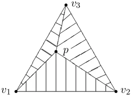
Figure 1. ch(v1, v2, v3) = ch(v1, v2, p)∪ch(v1, v3, p)∪ch(v2, v3, p).
4. {wij, wik, vS} fori∈S,
where i,j,k, l denote different integers, then V is contained in the sets of vertices ofPI(m) or one of the permutations of PII or PIII. This follows from a simple case analysis depending on
the number and kind ofwij’s inV.
Given any point p in the (closed) convex hull ch(V) of V, with p = Pv∈V avv, we can
write ch(V) = Sv:av>0ch((V\{v})∪ {p}). Indeed any point q in ch(V) can be written as
q =Pv∈V bvv=γp+Pv∈V(bv−avγ)v, where we can takeγ ≥0 to be such thatbv′ =av′γ for
somev′ witha
v′ >0 andbv ≥avγ for allv∈V. Now qclearly is a convex linear combination of
elements of (V\{v′})∪ {p}. This argument is visualized in Fig.1. As a generalization we obtain that if p∈ch(W) for some setW we have that ch(V)⊂Sv:av>0ch((V\{v})∪W).
Now we can consider a set of vertices V containing a bad configuration, and use the above method to rewrite ch(V)⊂Sich(Vi), where theViare sets of vertices ofP(m)that do not contain
that bad configuration, while not introducing any new bad configurations. Iterating this we end up with ch(V) ⊂Sich(Vi) for some sets Vi without bad configurations; in particular ch(V) is
contained in the right hand side of (5.1).
First we consider a bad set of the form{wij, wkl}. Thenp= 12(wij+wkl) = 12(vT1+vT2), where
T1andT2are any two sets of size|Ti|=m+1 withT1∪T2∪{i, j, k, l}={0,1, . . . ,2m+5}. Thus
we get V1 = (V ∪ {vT1, vT2})\{wij} and V2 = (V ∪ {vT1, vT2})\{wkl}, as new sets. In particular
the number of w’s decreases and we can iterate this until no bad sets of the form {wij, wkl}
exist.
For the remaining three bad kind of sets we just indicate the way a strictly convex combination of the vectors in the bad set can be written in terms of better vectors. In each step we assume there are no bad sets of the previous form, to ensure we do not create any new bad sets (at least not of the form currently under consideration or of a form previously considered).
1. For{wij, vS} withi, j∈S we have 23wij+13vS = 31(vT1+vT2+vU) where S\T1=S\T2 =
{i, j} andS∩U =T1∩U =T2∩U =∅and T1∩T2 =S\{i, j} (thusT1,T2 andU cover
all the elements of S, exceptiand j, twice, and all other points once).
2. For {wij, wik, vS} with i∈ S we have 13(wij+wik+vS) = 13(vT1 +vT2 +vU) for S\T1 =
S\T2 ={i}and S∩U =T1∩U =T2∩U =∅and T1∩T2=S\{i}and j, k6∈T1, T2, U.
3. For{wij, wik, vS} ⊂V, withi∈S, thenj, k6∈S and 13(wij+wik+vS) = 13(vT1+vT2+vU)
for S\T1 = S\T2 = {i} and S ∩U = T1∩U = T2 ∩U = ∅ and T1∩T2 = S\{i} and
j, k6∈T1, T2, U.
Let us now consider the bounding inequalities related to these polytopes.
Proposition 5.7. The polytopes P(m), PI(m), PII(m) and PIII(m) are the subsets of the hyperplane {α :α∈R2m+6|P
• For P(m) the bounding inequalities are
−12 ≤αi ≤1, (0≤i≤2m+ 5),
αi≤1 +αj+αk+αl, (|{i, j, k, l}|= 4),
αi−αj ≤1, (i6=j),
(|S| −2)αi+ X
j∈S
αj ≥0, (i6∈S,3≤ |S| ≤m+ 3).
For m= 0 the equations αr≤1 and αi ≤1 +αj+αk+αl are valid but not bounding. • The polytope PI(m) is described by the bounding inequalities
0≤αi≤1, (0≤i≤2m+ 5).
For this polytope too, if m= 0 the equations αr≤1 are valid but not bounding. • The polytope PII(m) is described by the bounding inequalities
−1/2≤α0,
αr−α0≤1, (r ≥1),
(|S| −2)α0+
X
j∈S
αj ≥0, (06∈S,0≤ |S| ≤m+ 3).
• Finally, the polytope PIII(m) is described by the bounding inequalities
αi+αj ≤0, (0≤i < j≤2),
−αi≤α0+α1+α2, (3≤i≤2m+ 5),
αi−1≤α0+α1+α2, (3≤i≤2m+ 5).
If m= 0 the equations αi−1≤α0+α1+α2 are valid but not bounding.
Proof . It can be immediately verified that the vertices of the polytopes P(m), PI(m), PII(m)
andPIII(m) satisfy the relevant inequalities, hence so does any convex linear combination of them. In particular it is clear that the polytopes are contained in the sets defined by these bounding inequalities.
Note that the different polytopes have symmetries of S2m+6 (for P(m) and PI(m)),
respec-tivelyS1×S2m+5 (PII(m)), respectively S3×S2m+3 (PIII(m)). We only have to find the bounding
inequalities of these polytopes intersected with a Weyl chamber of the relevant symmetry group, as all bounding inequalities will be permutations of these. These bounding inequalities can be written in the formµ·α≥0 for eachα in the polytope; we do not need affine equations as we have Prαr =m+ 1.
A bounding inequality must attain equality at a codimension 1 space of the vertices of the polytope; in particular if we consider all subsets V of 2m+ 5 vertices of the intersection of each polytope with the relevant Weyl chamber and insist on µ·v = 0 for each v ∈V, we find all bounding inequalities (and perhaps some more inequalities). For PI, PII and PIII we are in
the circumstance that there are 2m+ 6 vertices for the intersection of the Weyl chamber with the polytope; in particular each set of 2m+ 5 vertices corresponds to leaving one vector out. Moreover the sign of µis then determined by insisting on µ·v >0 for the remaining vertex v. As the equations are all homogeneous the normalization of µis irrelevant.
Let us consider the case ofPII. The set of relevant vertices is {vS, w01, e1−e2, . . . , e2m+4−
e2m+5} forS ={m+ 6, . . . ,2m+ 5}. We now have the following options for leaving one vector
1. If µ·vS(m)>0 we getµ=ρ+ (m+ 1)e0, thus the equationα0 ≥ −1/2.
2. If µ·w(01m)>0 we getµ=−e0 and the equationα0 ≤0.
3. If µ·(ei−ei+1)>0 for 1≤i≤m+ 3 we getµ = (i−2)e0+Pir=1er and the equation
becomes (i−2)α0+Pir=1er≥0.
4. If µ·ei−ei+1 >0 for m+ 4 ≤i ≤2m+ 4 we get µ = (m+ 2)(2m+ 5−i)e0+ (2m+
5−i)Pir=1er+ (m+ 4−i)P2r=mi+5+1er and the equation becomes (α0+ 1)(2m+ 5−i)≥
P2m+5
r=i+1αr.
Note that the equation α0 ≤0 is the|S|= 0 case of (|S| −2)α0+Pj∈Sαj ≥0. Now the last
set of equations all follow from the instance i= 2m+ 4, i.e. α0+ 1≥α2m+5 and the equation
α2m+5 ≥αr. The rest are true bounding inequalities. It is only hard to see that the solutions
to (i−2)α0+Pir=1er= 0 in the set of vertices of the polytope span a codimension one space;
however the set{w01, . . . , w0i} ∪ {vT |T ⊂ {i+ 1, . . . ,2m+ 5}}does span a set of codimension
one.
In a similar way one obtains the bounding inequalities forPI and PIII, we omit the explicit
calculations here. To obtain the bounding inequalities ofP itself, we observe that any bounding inequality ofP must be a bounding inequality of one ofPI,PII,PIII or one of their permutations,
as P is the union of those polytopes. Indeed any of these equations which are valid on P are bounding inequalities (as the span of the set of vertices for which equality holds does not reduce in dimension when going from a smaller polytope to P). Thus we can find the bounding inequalities for P by checking which of the bounding inequalities of these smaller polytopes are valid on P. This we only need to check on the vertices of P, which is a straightforward calculation.
Note that we could also have obtained the bounding inequalities forP in the same way that we obtained those ofPI,PII and PIII. However now we would have to take 2m+ 5 vectors from
the set{vS, w01, e0−e1, . . . , e2m+4−e2m+5}, which has 2m+ 7 elements. The number of options
therefore becomes quite large, thus we prefer to avoid this method.
We would like to give special attention to the bounding inequalities of P(1), which is the polytope which interests us most. We can rewrite these bounding inequalities in a clearly
W(E7) invariant way.
Proposition 5.8. The bounding inequalities forP(1) inside the subspaceα·ρ= 1 are given by
α·δ≤1, (δ∈R(E7)),
α·µ≤2, (µ∈Λ(E8), µ·ρ= 1, µ·µ= 4)
for α∈P(1). HereΛ(E
8) =Z8∪(Z8+ρ) is the root lattice ofE8.
Proof . Up toS8 one can classify the roots ofE7, givingδ =ei−ej orδ =ρ−ei−ej−ek−el,
which handles the bounding inequalities αi −αj ≤ 1 and αi +αj +αk +αl ≤ 0. Similarly
we can classify all relevant µ ∈ Λ(E8) as µ = 2ei, µ = ei +ej +ek −el, µ = ρ−2ei and µ=ρ+ei−ej−ek−el, the corresponding equations are again directly related to the bounding
inequalities of P(1) as given in Proposition5.7.
It is convenient to rewrite the integral limits of Propositions 4.1 and 4.2 in a uniform way which clearly indicates the bounding inequalities for the corresponding polytopes (i.e. PI, resp.
PIII). It is much harder to give such a uniform expression for PII (and we need separate
ex-pressions for the intersection with PI and PIII and the facet {α0 = 1 +α2m+5}), so we omit
Proposition 5.9. Define vectors vj =ej and wj =ej − m2+1ρ, then the bounding inequalities
Proof . These two propositions are just a rewriting of Propositions 4.1and 4.2.
With these expressions the proof of the following proposition becomes fairly straightforward.
Proposition 5.11. Let the polytope Q be either PI(m), PII(m) or PIII(m). For α ∈ Q the limit in (4.1) exists and depends only on the face ofQwhich contains α(i.e. ifα andβ are contained in the same face of Q thenBmα(u) =Bβm(u)).
Proof . Indeed Propositions 5.9, respectively 5.10 give the limits for the vectors α in PI(m), respectively PIII(m). For PII(m) the limits are given in Proposition 4.3, except for the cases with
α0 = 0 (which is the intersection with PI(m)), and α1+α2 = 0 (the intersection with PIII(m)), or
a permutation of such a case. In particular we have obtained limits in those cases as well. For PI and PIII the expressions in the previous two propositions immediately show that
the limits only depend on which bounding inequalities are strict or not, and hence on the face of the polytope containing α. For PII we note that the conditions α0 = 0 and α1 +
α2 = 0 (governing which proposition to look at) correspond to bounding inequalities. Within
Proposition 4.3 we observe that the condition αr = −α0 becomes a bounding equation once
2α0 = Pr≥1:α0+αr<0αr+α0 holds (as the difference of the equations with r ∈ S and with r 6∈ S). So also for PII the limit only depends on which bounding inequalities are strict and
which not.
We can now prove the first of the main theorems, the equivalent result for the full poly-tope P(m).
Proof of Theorem 5.2. By the S2m+6 symmetry of Em(t) we see that if a limit exists for
of PI(m), PII(m) and PIII(m), by the previous proposition we find that the limit Bmα exists for all
α∈P(m). We would like to extend the statement about dependence on faces as well. To prove
this it would be sufficient to show that all faces ofP(m)are in fact a face of one of the polytopes in its decomposition, however this is not true. We do have the following lemma.
Lemma 5.12. All faces of P(m) are faces of either PI(m), σ(PII(m)) or σ(PIII(m)) for some σ ∈ S2m+6, except the interior ofP(m) and permutations of the facet given by the equality α0+α1+
α2+α3 = 0.
Proof . Any face of P(m) can be written as the set of all convex linear combinations of some set V of vertices ofP(m). Recall that V is contained in the set of vertices ofPI,PII orPIII (or
a permutation thereof), unless it contains one of the four bad sets in the proof of Proposition5.6. Therefore, except whenV contains bad sets, the face determined byV is a face ofPI,PIIorPIII.
We now show that if V contains a bad set, the convex hull of V contains a point in the interior of P(m) or the interior of the facet given byα
0+α1+α2+α3 = 0. Hence ch(V) is either equal
to the interior of P(m), or to the special facet.
1. If {wij, vS1, vS2} ⊂ V (i∈ S1, j ∈S2) then (wij+vS1 +vS2)/3∈ ch(V). This is a point
where all elements are 1/6, 1/2 or 5/6, in particular it is a point in the interior of PI, and
thus of P itself.
2. If {wij, vS} ⊂V (i, j∈S), then (wij+vS)/2∈ch(V), which is in the interior ofPI.
3. If{wij, wik, vS} ⊂V, (i∈S), then (wij+wik+ 2vS)/4∈ch(V), which is again a point in
the interior of PI.
4. If{wij, wkl} ⊂V, then (wij+wkl)/2∈ch(V). All bounding inequalities ofP are strict on
this point exceptαi+αj+αk+αl = 0, thus it is a point in the interior of the corresponding
facet. Thus ch(V) is either this facet or the interior of P.
Now it remains to show that the function Bm
α is the same for all points in the interior, and all
points on the facet given byα0+α1+α2+α3= 0. This follows from the following lemma.
Lemma 5.13. On the facet of P(m) given by α
0 +α1 +α2 +α3 = 0 we have Bmα(u) =
(u0u1u2u3;q). Moreover on the interior of P(m) we have Bαm(u) = 1.
Proof . In the m = 0 case we find that the right hand side of the evaluation formula (3.2) converges for α on the facet to (q/u4u5;q) = (u0u1u2u3;q), while in the interior of P(m) the
limit converges to 1 (as for m = 0 the condition αr+αs = 1 is equivalent to the sum of the
other four parameters being zero.). Thus form= 0 the lemma is true.
Form >0 we can classify all the faces ofPI(m),PII(m)andPIII(m)which intersect the given facet
and the interior of P(m). The bounding inequality α0+α1+α2+α3 ≥0 implies that the only
vertices allowed in the closure of this facets are vS for 0,1,2,36∈S and wij fori, j∈ {0,1,2,3}.
We obtain the following set of faces ofPI,PIIandPIII in the facetα0+α1+α2+α3= 0 modulo
permutations of the parameters.
Polytope Vertices Relations
PI∩PII∩PIII vS (0,1,2,36∈S) α0 =α1=α2 =α3 = 0
PII∩PIII w01,vS (0,1,2,36∈S) α0 =α1=−α2=−α3
w01,w02,vS (0,1,2,36∈S) α0+α3= 0, α1 =α2= 0
PII w01,w02,w03,vS (0,1,2,36∈S) α0 < αr<−α0 (r = 1,2,3)
We omitted the conditions on αr for r ≥ 4 as they are the same in each case. Indeed the
bounding inequalities imply that −β < αr <1 +β for r ≥4, where β is the sum of the three
smallest parameters. The classification becomes apparent once we realize that thevS part of the
vertices of the faces is fixed (they must contain a point vS with 0,1,2,3 6∈S to be in the open
facet, while they cannot contain any other vS). Thus we only have to consider the possibilities
for adding some wij’s. In these five faces we can directly check what the limit is, and observe
that the corresponding integrals and sums indeed evaluate to the desired (u0u1u2u3;q). The
required evaluation identities are provided by them= 0 cases of these faces.
Similarly we can describe all faces of PI, PII and PIII (modulo permutations) meeting the
interior of P.
Polytope Vertices Relations
PI∩PII∩PIII vS, (0,1,26∈S) α0 =α1 =α2= 0
PI∩PII vS (0,16∈S) α0 =α1 = 0< α2<1
vS (06∈S) α0 = 0< α1, α2 <1
PI vS 0< α0, α1, α2<1
PII∩PIII w01,vS (0,1,26∈S) −1/2< α0 =α1=−α2
w01,w02,vS (0,1,26∈S) −1/2< α0 < α1=−α2
PIII w01,w02,w12,vS (0,1,26∈S) αr+αs <0, (r, s∈ {0,1,2})
PII w01,vS (0,1,6∈S) −1/2< α0 =α1>−α2
w01,w02,w03,vS (06∈S) α0 <0 andα0 < α1 >−α2
For each face we have the extra conditions−β < αr<1 +β for r≥3. We can check for all
these 9 faces that the value on that face equals 1 identically. Again the required evaluations all
follow from them= 0 case.
We conclude that also on the two types of faces ofP(m) which are not a face of one of the
subpolytopes, the value is the same on the entire face.
We can now also prove the second main theorem, the iterated limit property.
Proof of Theorem 5.3. It is sufficient to prove this property for the closed polytopes PI(m),
PII(m) and PIII(m). Observe that for the vectortα+ (1−t)β precisely those boundary conditions (of the respective polytopes) are strict which are strict for either α orβ.
In Propositions 5.9 and 5.10 we have written the limits in PI and PIII as an integral of
a product of terms f(u, w) = (uw;q)1{w·α=0} where w·α ≥ 0 is the sum of some bounding
inequalities. In particular in the expression forBtαm+(1−t)βonly those terms remain corresponding to sums of bounding inequalities which are attained in both α and β. On the other hand, as (xβ−αu)w =x(β−α)·wuw we find that ifw·α=w·β= 0 then the termfα(xβ−αu, w) is constant
in x and thus does not change in the limit, while ifw·α > 0, we find that fα(xβ−αu, w) = 1
is again independent of x, and finally if w·α = 0 < w·β, then we have a uniform limit limx→0fα(xβ−αu, w) = limx→0(xβ·wuw;q) = 1 =ftα+(1−t)β(u, w). Thus to prove iterated limits
we only have to show we are allowed to interchange limit and integral, which follows from the fact that we integrate over some compact contour, and the fact that the x-dependent poles which have to remain inside the contour converge to 0, while the x-dependent poles which have to remain outside the contour go to infinity; in particular for x small enough we can take an
x-independent contour.
To prove the result forPIIis more complicated as we do not have a uniform description of the
limit. For the closed facets determined by α0 = 0, α1+α2 = 0 or α0 =α1 we have an integral
description (see Propositions 4.1, 4.2 and 4.4), and limits within these facets can be treated as for PI and PIII. For the complement of these facets the limit is given in Proposition 4.3 as
sums instead of integrals to see that iterated limits within the complement of the facets hold. We are left with showing that limits from one of the three facets to the inside behave correctly. These limits all pass from an integral to a single sum. The simplest argument we found is to simply calculate these limits in all three cases separately (due to the rather uniform expressions of the integrals and single sums, we can handle the different faces in each of the closed facets uniformly). It boils down to picking the residues associated with poles which either go to zero as x → 0, while they should be outside the contour, or go to infinity while they should be inside the contour. Subsequently we bound the integrand around the unit circle to show that the remaining integral vanishes in the limit. Finally we give a bound on the residues and use dominated convergence to show we are allowed to interchange limit and sum. This bound also serves to show that the sum of the residues which are not associated to u0 (where we take the
first coefficient in α to be the strictly lowest one) vanishes as well. The calculations involved are again tedious, and very similar to the calculations in the proof of Proposition 4.3.
6
Transformations: the
m
= 1 case
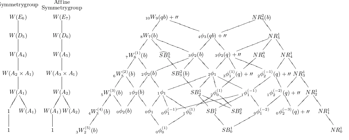
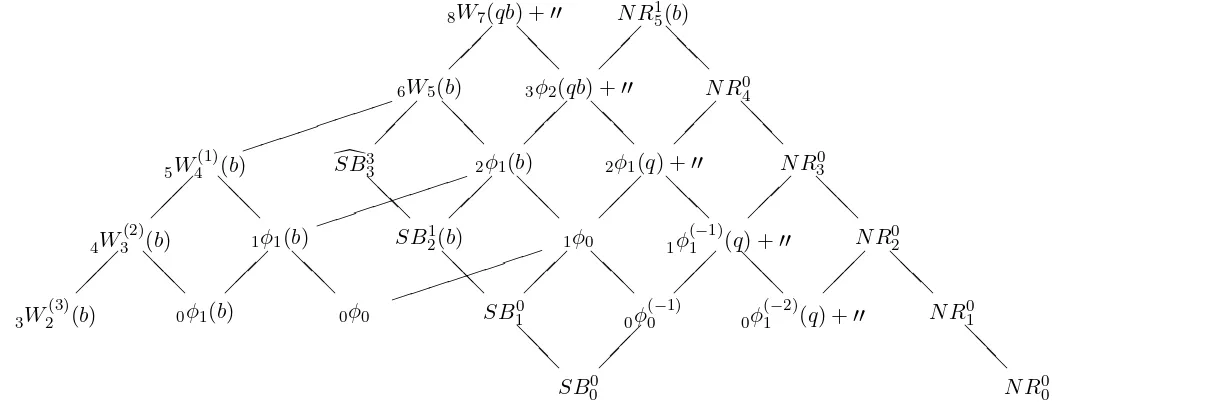
In this section we start harvesting the results we can now immediately obtain given this picture of basic hypergeometric functions as faces of the polytope P(1). This was already done for the top two levels (i.e. the functions corresponding to vertices and edges) by Stokman and the authors in [1], though there we did not yet see the polytope. In the next section we give a worked through example (related to2φ1) of the abstract results in this section. As a convenient tool to
understand the implications of the results mentioned, we refer to Appendix A which contains a list of all the possible functions Bα1.
Recall that we have a basic hypergeometric function attached to each face of the polytopeP(1), and that the Weyl groupW(E7) acts both on P(1) and on sets of parameters ˜H1. As the elliptic
hypergeometric function is invariant under this action we immediately obtain
Theorem 6.1. Let w∈W(E7), α∈P1 and u∈H˜1 then
B1α(u) =Bw1(α)(w(u)).
Proof . Indeed we have
B1α(u) = lim
p→0E
1(pα·u) = lim p→0E
1(w(pα·u)) = lim p→0E
1(pw(α)·w(u)) =B1
w(α)(w(u)).
This gives us formulas of two different kinds for the functions B1α.
First of all we can obtain the symmetries of a function by considering the stabilizer of the corresponding face with respect toW(E7). This includes for example Heine’s transformation of
a2φ1, transformations of non-terminating very-well-poised8φ7’s, and Baileys’ four-term relation
for very-well-poised 10φ9’s (as a symmetry of a sum of two 10φ9’s).
The symmetry group of the related function is the stabilizer of a generic point in the face, or equivalently the stabilizer of all the vertices of the face. Indeed if some element of w fixes the face, but non-trivially permutes the vertices of the face, then it can be written as the product of a permutation of the vertices generated by reflections in hyperplanes orthogonal to the face, and a Weyl group element which stabilizes the vertices of the face. However, as the functionsB1α(u) only depend on the space orthogonal to the face, the first factor has no effect.
Secondly, elements of the Weyl group which send one face to a different face induce trans-formations relating the two functions associated to these two faces. Examples of this include Nassrallah and Rahman’s integral representation of a very-well-poised 8W7, the expression of
this function as a sum of two balanced 4φ3’s, and a relation relating the sum of two3φ2’s with
Indeed all simplicial faces ofP(1) of the same dimension are related by theW(E7) symmetry,
except for dimension 5. Indeed for dimension 5 there are two orbits: 5-simplices which bound a 6-simplex and those which do not. In particular in Fig. 2 below, there exist transformation formulas between all functions on the same horizontal level, except for the second-lowest level, where you must distinguish between those faces which are at the boundary of some higher dimensional simplicial face, and those that are not. As two functions between which there exists a transformation formula have the same symmetry group, we have written down the symmetry groups of all the functions on each level on the left hand side. Note that the symmetry group for 5-simplices at the boundary of a 6-simplex is 1 (i.e. the group with only 1 element), while for the other 5-simplices the symmetry group is W(A1)∼=S2.
We can also consider the limit of the contiguous relations satisfied byE1. Theq-contiguous
relations reduce toq-contiguous relations. We get a relation for each set of three termsBα(u·qβi),
where the βi are projections of points in the root lattice of E7 to the space orthogonal to the
face containing α.
More interesting is the limit of a p-contiguous relation. In order for us to be able to take a limit we have to find three points onP1 whose pairwise differences are roots of E7.
Proposition 6.2. Let α, β, γ ∈ P(1) be such that α−β, α−γ, β −γ ∈ R(E7) and form an
equilateral triangle(i.e.(α−β)·(α−γ) = 1), and letu∈H˜1. RecallS ={v∈R(E8)|v·ρ= 1}.
Then
Y
δ∈S δ·(α,β,γ)=(1,0,0)
(uδ;q)uγθ(uβ−γ;q)B1α(u) + Y
δ∈S δ·(α,β,γ)=(0,1,0)
(uδ;q)uαθ(uγ−α;q)Bβ1(u)
+ Y
δ∈S δ·(α,β,γ)=(0,0,1)
(uδ;q)uβθ(uα−β;q)Bγ1(u) = 0. (6.1)
Note that (6.1) is written in its most symmetric form. In order to avoid non-integer powers of the constants one should first multiply the entire equation by u−α and useuρ=q.
Proof . Choose ζ such that ˜α =α+ζ, ˜β = β+ζ and ˜γ = γ+ζ are all roots of E7. This is
possible by choosing ˜α such that ˜α·(α−β) = 1 and ˜α·(α−γ) = 1, and we can always find roots satisfying these two conditions. Now observe that ˜α·β˜ ≤ 1 as inner product of two different roots ofE7, and that
˜
α·β˜= (α+ζ)·(β+ζ) = (α+ζ)·(α+ζ) + (α+ζ)·(β−α)≥2−1 = 1,
asα+ζ 6=−(β−α) (equality here would implyβ+ζ = 0). Thus ˜α·β˜= 1, and hence ˜α, ˜β and ˜
γ satisfy the conditions of Theorem3.5. Setting t=u·pζ in (3.3) we obtain Y
δ∈S δ·(α−β)=δ·(α−γ)=1
(uδpδ·β;q)uγpγ·ζθ(uβ−γpζ·(β−γ);q)E1(u·pα)
+ Y
δ∈S δ·(β−α)=δ·(β−γ)=1
(uδpδ·γ;q)uαpα·ζθ(uγ−αpζ·(γ−α);q)E1(u·pβ)
+ Y
δ∈S δ·(γ−α)=δ·(γ−β)=1
(uδpδ·α;q)uβpβ·ζθ(uα−βpζ·(α−β);q)E1(u·pγ) = 0. (6.2)
foru∈H˜1. Now we prove a lemma
Lemma 6.3. Let α,β and γ be as in the Proposition and let δ ∈S satisfy δ·(β−γ) = 0 then
Proof . Recall the bounding inequalities for P(1) given in Proposition 5.8. Note that µ =
ρ−γ+β−δ∈Λ(E8) satisfies µ·ρ= 1 and µ·µ= 4, thus we get β·(ρ−γ+β−δ)≤2 and
similarlyγ·(ρ+γ−β−δ)≤2. Adding these two inequalities and simplifying givesδ·(β+γ)≥0, and as (β−γ)·δ = 0, this implies δ·β ≥0.
Now observe that
ζ·(β−γ) = ( ˜α−α)·(β−γ) = ˜α·( ˜β−˜γ)−α·(β−γ) =−α·(β−γ),
where in the last equality we used that ˜α·β˜= 1 = ˜α·γ˜. Thus we need to show thatα·(β−γ) = 0. By the bounding inequalities we haveα·(α−β)≤1, but also
α·(α−β) = (α−β)·(α−β)−β·(β−α) = 2−β·(β−α)≥1.
Thus we find α·(α−β) = 1. By symmetry we also have α·(α−γ) = 1. Thus it follows that
α·β=α·γ, orα·(β−γ) = 0.
The lemma shows that pγ·ζ =pα·ζ =pβ·ζ, so we can divide by this term. Using this lemma
we see that we can subsequently take the limit p → 0 in (6.2) directly as the arguments of the θ functions do not depend on p, while the arguments of the q-shifted factorials are either
independent of por vanish as p→0.
The relations obtained in this way are three-term relations. By the geometry of the polytope the α,β and γ in the above proposition must be such that the faces they are contained in, are in the same W(E7) orbit. In particular we can rewrite our three term relation as a relation
between three instances of the same function. Thus we get as examples three-term relations for
3φ2’s [6, (III.33)]. Moreover we obtain the six-term relations of10φ9’s as studied in [7] and [9].
One reason why the p-contiguous relations morally should exist on the elliptic level is that the three functions related by p-shifts in roots of E7 satisfy the same second order q-difference
equations (after a suitable gauge transformation). In particular we can take the limit of theseq -difference equations and see thatBα1,B1β andB1γalso satisfy the same second order q-difference equations. In a very degenerate case, there exist faces for which to a vector αin that face there exists exactly one rootr ∈R(E7) suchα+r ∈P(1). In particular, while we cannot find a three
term relation in this case, we do obtain the second solution of the corresponding q-difference equations. In the general case we can obtain the symmetry group of theq-difference equations by looking at the stabilizer of the shifted lattice α+ Λ(E7) for a generic point α in the face.
This stabilizer, the stabilizer of α under theaffineWeyl group, is denoted the affine symmetry group in Fig. 2.
7
An extended example:
2φ
1In this section we consider the simplicial face with verticesw01,w02,v67andv57. The centroid of
this face is the point α= (−1/4,0,0,1/4,1/4,1/2,1/2,3/4), and we find using Proposition 4.2 that the limit can be expressed as
B1α(u) = (q, u3u0, u4u0;q)
(q/u1u2;q)
Z
θ(u0u1u2/z;q)
(qz/u7;q)
(u0/z, u3z, u4z;q)
dz
2πiz
= (u1u2, qu0/u7;q)2φ1
u0u3, u0u4
qu0/u7 ;q, u1u2
,
as long as this series converges (this integral expression for a 2φ1 is not very exciting, as it is
The stabilizer group of this face under the W(E7) action equals the stabilizer of α (as it
should be a permutation of the four vertices of the face). However those reflections in W(E7)
which non-trivially permute the vertices of the face are in roots which are the difference of two vertices, so they will just induce a shift along a vector in the face; as our functions only depend on the space orthogonal to the face, they act as identity on our function (for example they permute u1 ↔ u2 or u5 ↔ u6). Thus we are only interested in those elements of W(E7)
which leave the four vertices of this face invariant. In particular, this includes (and by Coxeter theory, is generated by) the reflections in the hyperplanes orthogonal to the roots {±(e3 −
e4),±(ρ−e0−e3−e4−e7),±(ρ−e0 −e3 −e5−e6),±(ρ−e0−e4−e5−e6)}. These eight
another one of Heine’s transformations [6, (III.2)]. Together with the permutation swappinga
and b (given byse3−e4) these two transformations generate the entire symmetry group.
As for transformations to other functions, there are no less than 6 other faces in theW(E7
)-orbit of the face containing α up to S8 symmetry. The related transformations are given by
(after some simplification)
Let us now consider the three term relations (as limit ofp-contiguous relations). The pointsβ
β Bβ1
parameters. Any three of these four functions now give a three term relation, for example (after simplification)
The affine symmetry group is now given as the extension of the symmetry group by also allowing elements which permute the four 2φ1’s amongst themselves. Indeed the index [W(A3 ×A1) :
W(A2×A1)] = 4. It is also the symmetry group of the q-difference equations we discuss next.
The q-contiguous equations relate three terms of the form Bα1(u ·qβ) where β is in the projection Λα of Λ(E7) on the space orthogonal to the face containing α. In particular the
lattice Λα is generated by (π denotes the orthogonal projection on Λα)
π(0,0,0,1,0,−1,0,0) = (1/4,0,0,3/4,−1/4,−1/2,−1/2,1/4), π(0,0,0,0,1,−1,0,0) = (1/4,0,0,−1/4,3/4,−1/2,−1/2,1/4), π(0,0,0,0,0,1,0,−1) = (1/4,0,0,−1/4,−1/4,1/2,1/2,−3/4), π(0,0,1,0,0,−1,0,0) = (0,1/2,1/2,0,0,−1/2,−1/2,0).
If we simplify 2φ1 by setting a=u0u3, b=u0u4, c=qu0/u7 and z =u1u2, these four vectors
correspond to multiplying respectivelya,b,c, orzbyq. In particular we have a relation for any three sets of parameters wherea,b,candz’s differ by an integer power ofq. For example using shifts π(ρ−e2−e4−e5−e6),π(e1−e5) andπ(e1−e2) (corresponding toa7→aq,z7→qz and
8
Evaluations: the
m
= 0 case
In the m = 0 case the general polytope picture is somewhat unsatisfying as a description of the possible limits of the elliptic hypergeometric beta integral evaluation. Indeed there are two issues. First of all the polytopeP(0)as described in Section5is not the entire polytope for which