The joint demand for cigarettes and marijuana:
evidence from the National Household Surveys on
Drug Abuse
Matthew C. Farrelly
∗, Jeremy W. Bray, Gary A. Zarkin,
Brett W. Wendling
Center for Economics Research, Research Triangle Institute, 3040 Cornwallis Road, Research Triangle Park, NC 27709, USA
Received 1 January 1999; received in revised form 1 June 2000; accepted 5 June 2000
Abstract
Recent studies have shown that efforts to curb youths’ alcohol use, such as increasing the price of alcohol or limiting youths’ access, have succeeded but may have had the unintended consequence of increasing marijuana use. This possibility is troubling in light of the doubling of teen marijuana use from 1990 to 1997. What impact will recent increases in cigarette prices have on the demand for other substances, such as marijuana? To better understand how the demand for marijuana and tobacco responds to changes in the policies and prices that affect their use, we explore the National Household Survey on Drug Abuse (NHSDA) from 1990 to 1996. We find evidence that both higher fines for marijuana possession and increased probability of arrest decrease the probability that a young adult will use marijuana. We also find that higher cigarette taxes appear to decrease the intensity of marijuana use and may have a modest negative effect on the probability of use among males. © 2001 Elsevier Science B.V. All rights reserved.
JEL classification:I1
Keywords:Marijuana; Cigarettes; Price; Complements; Elasticity; Demand
1. Introduction
Marijuana use among youths continues to rise despite community, state, and national efforts to educate and inform individuals of the harmful effects of drug use and abuse. For example, between 1990 and 1997, marijuana use among 12–17-year-old more than doubled,
∗Corresponding author. Tel.:+1-919-541-6852; fax:+1-919-541-6683.
E-mail address:[email protected] (M.C. Farrelly).
increasing from a prevalence of 4.4–9.7% (SAMHSA, 1998). The dramatic increase in marijuana use poses new challenges to decision makers developing policies to curb drug use among youths. During this same time period, current cigarette use has steadily increased among 8th, 10th, and 12th graders (MTF, 2000). Epidemiological studies indicate that licit drug use (e.g. tobacco and alcohol) may serve as a gateway to illicit drug use (Kandel, 1975; Kandel and Faust, 1975; Kandel and Yamaguchi, 1993; Duncan et al., 1998). If cigarette use is a gateway to marijuana use, recent policies directed at curbing current youth smoking may also lead to declines in marijuana use. Other studies have demonstrated interdependence between policies directed at curbing alcohol and marijuana use (DiNardo and Lemieux, 1992; Model, 1993; Chaloupka and Laixuthai, 1997; Pacula, 1998a,b).
All of these studies emphasize the importance of understanding the interdependence of widely used substances, such as alcohol, tobacco, and marijuana and suggest that policies affecting one substance may have unintended consequences on the others. Understanding these interdependencies is especially relevant in light of the US$ 0.45-per-pack cigarette price increase announced in November 1998 in response to the US$ 206 billion tobacco industry settlement with 46 states. Policy makers must understand whether proposals in-tended to reduce smoking among youths have uninin-tended consequences among youths and the general population that may cause marijuana use and other substance use to rise.
The goal of this paper is to further explore the interdependencies between tobacco and marijuana using a rich database on drug use, the National Household Survey on Drug Abuse (NHSDA). The NHSDA is a nationally representative survey of the US nonin-stitutionalized population aged 12 and older. The detailed questions on substance use contained in the NHSDA allow us to better understand how marijuana use responds to changes in policies that affect the price and availability of marijuana and tobacco. We focus our analyses on youths aged 12–20. We chose this age group for several reasons. Recent trends show dramatic changes in marijuana use for youths aged 12–20 but not for adults aged 21–30. Also, many children first experiment with tobacco and marijuana in their teens.
variables may bias the coefficients on the policies and price variables, all marijuana and tobacco models include state fixed effects.
The results of this paper will help guide the creation of comprehensive policies that curb the use of marijuana in two ways. First, we quantify the effects of policies aimed at curbing the use of marijuana, allowing policy makers to evaluate alternative policy options. For example, we provide estimates of the impact of police efforts to enforce marijuana possession laws and the impact of state-level marijuana possession fines. Second, we present results that clarify the cross-price effects between tobacco demand and marijuana use. With an understanding of this interdependency, policy makers can take into account how policy changes directed at one substance affect the demand for the other.
2. Previous studies
In this section, we discuss previous studies that have examined the interdependence of marijuana and tobacco use. There is an extensive literature on the relationship between cigarette and marijuana use, focusing primarily on tobacco use as a ‘gateway’ to other drug use, including marijuana. Cigarette smoking is considered a gateway drug by some because youths who start with tobacco and alcohol use are more likely to progress to marijuana and other drug use (Kandel, 1975; Kandel and Faust, 1975; Ellickson et al., 1992; Kandel and Yamaguchi, 1993; Duncan et al., 1998). The seminal work by Denise Kandel in 1975 involved tracking licit and illicit drug use by 7250 high school students in New York over a 2-year period. Kandel divides drug use into six categories — legal drugs, marijuana, pills, LSD, cocaine, and heroin — and finds that drug use tends to be cumulative. In other words, youths in any one category have used all ‘lower-ranked’ drugs. In subsequent work, Yamaguchi and Kandel (1984) find that current alcohol and cigarette use are both strong predictors of initiation of marijuana use. In more recent work, Duncan et al. (1998) find that cigarettes are a stronger predictor of future marijuana use than alcohol and that higher levels of cigarette use are predictive of greater future marijuana use.
From a physiological perspective, two studies suggest that marijuana may be a substitute for cigarettes among current users of both substances. Simmons and Tashkin (1995) ob-tained detailed marijuana and cigarette smoking histories from 467 adult regular smokers of marijuana and/or cigarettes and found that those who smoke both cigarettes and marijuana smoke significantly fewer cigarettes per day than those who do not smoke marijuana. How-ever, marijuana use is not significantly different for smokers and nonsmokers of cigarettes. Of those who smoke both, 49% began smoking cigarettes first, while 33% smoked marijuana first. Similarly, a controlled experiment of current marijuana and cigarette users illustrates the interdependence of marijuana and cigarettes among current users. Kelly et al. (1990) find that active marijuana smoking (placebo versus active marijuana cigarettes were used) significantly decreased the number of daily cigarette smoking bouts, increased inter-bout intervals, and decreased inter-puff intervals. Although these studies illustrate the potential correlation between marijuana and tobacco, they are both based on relatively small samples of subjects.
policies can affect the use of the targeted substance as well as potentially related substances (DiNardo and Lemieux, 1992; Model, 1993; Thies and Register, 1993; Chaloupka and Laixuthai, 1997; Pacula, 1998a,b; Saffer and Chaloupka, 1998; Chaloupka et al., 1999). However, among these studies, only three have examined the relationship between mari-juana and tobacco (Pacula, 1998a,b; Chaloupka et al., 1999). A limitation of all of these studies is that they lack data on the price of marijuana and hence must rely on proxies for the price of marijuana.The only readily available data on the price of marijuana come from Drug Enforcement Administration databases. These databases capture purchases made by undercover federal agents nationwide and police officers in Washington, DC. Because fed-eral interdiction efforts focus primarily on cocaine, heroin, methamphetamines, and other illicit substances other than marijuana, there are relatively few price observations for mari-juana in any 1 year in a given city, with the notable exception of Washington, DC. For example, between 1988 and 1997, there were an average of 44 price observations for DC, but only three observations on average in other states. For this reason, this and previous studies do not include the price of marijuana.
In the only published article on the relationship between marijuana and tobacco use, Pacula (1998a) analyzes the 1984 wave of the National Longitudinal Survey of Youth (NLSY) to estimate the joint demand for alcohol and marijuana using a sample of roughly 8000 individuals. Pacula estimates separate demand models for alcohol and marijuana demand and shows that increasing beer taxes decreases the prevalence and consumption of alcohol and decreases the prevalence of marijuana use. She also finds that respondents are more likely to use marijuana in states that have decriminalized marijuana and less likely to use marijuana in states with relatively high cigarette taxes. However, neither of these results is statistically significant.
In a continuation of this research, Pacula (1998b) analyzes two waves of the NLSY and estimates the effect of current and past cigarette prices on current marijuana use. She finds that the two substances are economic complements — higher current and past prices reduce the probability of current marijuana use.
Finally, in a recent working paper by Chaloupka et al. (1999), the authors examine the relationship between marijuana and tobacco use by 8th-, 10th-, and 12th-graders, using cross-sectional data from the 1992–1994 Monitoring the Future Surveys (MTF). They find that higher cigarette prices lead to a decrease in the probability and frequency of marijuana use. Surprisingly, the respective cross-price elasticities are−0.73 and−0.84, for a total elasticity of−1.57. This is larger than the own-price elasticities from their cigarette demand equations, which yielded a participation elasticity of −0.42 and a conditional demand elasticity of−0.71, for a total cigarette price elasticity of−1.13.
In summary, the results of these studies provide some evidence that marijuana and tobacco are economic complements. However, it is difficult to draw strong conclusions from these studies for two reasons. First, all three studies that focus on marijuana and tobacco use rely on relatively few years of time-series cross-sectional data, which limits the variation in cigarette prices. Second, because of the limited number of cross-sections, none of these studies controlled for unobserved, state-specific characteristics. In the absence of state fixed effects, it is unclear whether the estimated effects reflect the preferences of individuals in the state or capture the effect of an exogenous policy change. For example, these studies rely on an indicator variable for states in which marijuana is decriminalized, without controlling for state fixed effects. It is not clear whether this indicator variable captures the effect of decriminalization on use or other state-specific characteristics that may be correlated with use, such as the willingness to accept alternative behaviors or lifestyles. The same may be true for cigarette prices, because they too may capture unobserved characteristics of the state. Failing to control for these unobserved characteristics may bias the estimate of the effects of all state policy and price variables.
The purpose of this paper is to examine the effects of cigarette taxes and nonprice mari-juana policies on both marimari-juana and cigarette use. We are able to control for state effects using 7 years of pooled cross-sections and have a richer database of marijuana policies than have been used before. To proxy for the price of marijuana, we constructed an annual measure of the probability of being arrested for marijuana possession in each state. In addi-tion, for selected years, we collected data on state fines and jail terms for violations of state marijuana laws to proxy for the price of marijuana. By including these state policies and state fixed effects, we are better able to distinguish the effects of state policies and prices from the effects of unobserved state characteristics. Finally, given the changes in cigarette tax policies across states and over time between 1990 and 1996, we are able to identify the effects of cigarette taxes on both the probability and frequency of marijuana use.
3. Data
In this study, we used data from the NHSDA. The NHSDA is a key national indicator of the nation’s drug use behavior and problems. The National Institute on Drug Abuse (NIDA) sponsored the NHSDA from 1974 to 1992, and the Substance Abuse and Mental Health Services Administration (SAMHSA) has sponsored the surveys since 1992. The NHSDA is designed to provide data on the extent of drug use and abuse by the noninstitutionalized civilian population aged 12 and older in the US (SAMHSA, 1992, 1994).
We combined data from the 1990–1996 NHSDA to provide estimates of the own- and cross-price and policy effects on the demand for marijuana and tobacco. The NHSDA used identical survey questions in all 7 years for the prevalence of past-month use of marijuana and tobacco and the same five-stage area probability sample design. Sampling weights were computed based on the probability of selection at each stage, and these weights were used in all analyses.
sub-stance use, which is a potential limitation of self-reported surveys (Hoyt and Chaloupka, 1993). In a 1990 field test of various survey instruments, Turner et al. (1992) found that the self-administered format of the NHSDA decreases the underreporting of substance use compared to an interviewer-administered format. The NHSDA was revised in 1994 so that tobacco use questions were also reported using a self-administered questionnaire, resulting in some noncomparability of pre- and post-1994 estimates. In particular, youth tobacco use increased dramatically as a result of this change. For this reason, we include an additional indicator variable for the 1994–1996 surveys in the youth tobacco demand equations.
Although the NHSDA is the only survey that provides detailed and consistent data on drug use among members of the household population in the coterminous US, the NHSDA has a number of limitations. First, as mentioned above, the data are self-reports of drug use, so their value depends on respondents’ truthfulness and memory. Although the self-administered format of the NHSDA decreases the underreporting of substance use in general, any given individual’s propensity to report substance use may be affected by the degree of privacy during the interview. To examine the sensitivity of our results to the degree of privacy, we include the interviewer’s report of the degree of privacy during the interview as a supplemental covariate in our demand equations. The interviewer indicates the degree of privacy on a scale from 1 (completely private) to 9 (constant presence of another). We included an indicator that represented no significant interruptions (value of 4 or less).
Second, a small proportion (roughly 1%) of the US population is excluded from the surveys. With the exception of 1991, the subpopulations excluded are those residing in non-institutional group quarters (e.g. military installations, college dormitories, group homes), those in institutional group quarters (e.g. prisons, nursing homes, treatment centers), and those with no permanent residence (e.g. the homeless and residents of single rooms in ho-tels). In 1991, the target population was extended to all 50 states and included residents of noninstitutional group quarters and civilians living on military bases. If the drug use of excluded groups differs from that of the household population, the NHSDA may provide slightly inaccurate estimates of drug use in the total population. This may be particularly true for the homeless and prison populations.
3.1. Analysis variables
The dependent variables used in our analyses include indicator variables for any past-month use of marijuana, any past-month use of cigarettes, the frequency of marijuana use in the past 30 days (1–30 days) conditional on use, and cigarettes per day conditional on use. The demographic controls used in our analyses are all self-reported measures from the NHSDA public use files. These controls consist of gender, age, number of people living in the household, number of children under age 12 in the household, marital status, race, family income, current school enrolment status, education, and size of the metropolitan statistical area (MSA) of residence. In addition to these self-reported variables, we also included two interviewer-reported variables: urban/rural status of the respondent’s current residence and an indicator for the degree of privacy during the interview.
terms for marijuana possession law violations. Unlike other studies, we do not include an indicator for states that have decriminalized marijuana possession because there is essen-tially no variation in this variable within states over time during 1990–1996. In addition, the concept of decriminalization is subsumed in our data on state marijuana possession fines.
Marijuana possession arrest data for youths and adults come from county-level Uniform Crime Reports for 1990–1996. Using these data and marijuana use data from the NHSDA, we created two measures of the probability of being arrested. The first measure is the state marijuana possession arrests for youth divided by the number of current marijuana users aged 12–20 in that state. This measure provides an estimate of the probability of being arrested for youth. The second measure is similar to the first but is calculated for all ages 12 and older, not just youth, by dividing the total marijuana possession arrests for all ages in a state by the number of marijuana users in that state. For both age groups, state-level measures of marijuana use were estimated by taking the weighted prevalence of current marijuana use state-by-state. We then multiplied this prevalence by the population in the respective age group from the NHSDA to estimate the total number of users in a state. The purpose of the first measure is to have a youth-specific measure of the probability of arrest. However, because the denominator, youth state marijuana use, may induce some negative correlation with the dependent variable in the marijuana demand equations, we also use the second measure for all ages to provide a lower and upper bound of the results.
Because the NHSDA was not designed during this time period to support state repre-sentative data, some states have small samples (therefore, state-level estimates will not be reported). The limited sample sizes should only increase the standard errors of our estimates and not bias our results of the effect of the probability of arrest on use.1
We also have state marijuana law data on fines for various quantities of marijuana posses-sion for 1990–1996 that we collected from state legal code books. The marijuana possesposses-sion laws specify the minimum and maximum monetary fines and jail terms for varying amounts of marijuana possession. In other words, states usually specify fines and penalties for an ounce of marijuana and then another set of penalties for some larger quantity. To charac-terize these penalties and document changes in the levels of fines within states over time, it is necessary to obtain the legislative histories of the state laws. This is a research-intensive process. We were able to successfully code all states with the exception of North Carolina, North Dakota, and Tennessee for 1990–1996 and New Hampshire, New York, Rhode Island, and Vermont for 1990–1993. Observations for these states and years were dropped from the analysis.
Characterizing state marijuana laws also poses some challenges not only because the penalties for possession of a given quantity vary from state to state, but also because there is not a standard schedule of quantities that trigger increased sanctions. In essence, the marijuana penalties in each state form a step function where, for example, between any positive quantity and 1 pound, some states may have three distinct penalty levels, while
1In previous specifications, we used total state marijuana arrests divided by total arrests as a proxy measure for
others have only one. To capture these differences, we chose to estimate models with the minimum and maximum penalties for the first and second quantity categories (e.g. typically any positive quantity up to 1 ounce and then 1–4 ounces). In addition to these measures, we include a variable that indicates the height or change in the penalty of this first step and an indicator variable for states with only one level of penalties for all quantities. To reduce the potential for multicollinearity, we chose a final specification that includes the average of the minimum and maximum penalties for each quantity.
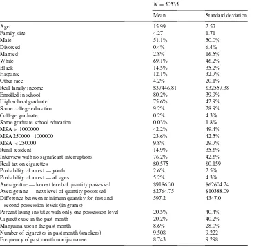
Data on cigarette excise taxes and prices come from the Tax Burden on tobacco, an annual report from the Tobacco Institute that contains state-level information on state and federal excise taxes and average state cigarette retail prices (Tobacco Institute, 1997). Summary statistics (mean and standard deviation) of both NHSDA survey data and state-level policy and price data are listed in Table 1.
Table 1
Descriptive statistics for ages 12–20, NHSDA 1990–1996
N=50535
Interview with no significant interruptions 76.2% 42.6%
Real tax on cigarettes $0.575 $0.159
Probability of arrest — youth 2.6% 2.5%
Probability of arrest — all ages 5.2% 4.3%
Average fine — lowest level of quantity possessed $9186.30 $62604.24 Average fine — next level of quantity possessed $2764.75 $10388.09 Difference between minimum quantity for first and
second possession levels (in grams)
597.2 4347.0
Percent living in states with only one possession level 20.5% 40.4%
Cigarette use in the past month 20.2% 40.2%
Marijuana use in the past month 8.6% 28.0%
Number of cigarettes in past month (smokers) 9.508 9.222
4. Methods
This section describes our study methodology using pooled independent cross-sections of the 1990–1996 NHSDAs. Because we are concerned with the contemporaneous effects of prices and policies on marijuana and tobacco use, we define current users of marijuana and cigarettes as those who have had any use in the past month.
In this paper, we focus on the decision to use marijuana and the frequency of marijuana use in the past month, defined as the number of days of any use. To address the impact of cigarette taxes and policies on marijuana use, we estimate the following demand specifica-tion for marijuana:
prob(M >0)=Φ(β0+β1+β2Year+β3State+β4PMM+β5PMC) (1) whereMis current marijuana use (past 30 days),Φthe standard normal cumulative density function, andXa vector of the sociodemographic variables described above.PMM repre-sents the effect of the marijuana ‘price’ variable where price is measured by the probability of being arrested for marijuana possession, andPMCis the price of cigarettes (using state excise taxes). We expect the sign ofβ4to be negative so that as the probability of getting arrested increases, individuals will be less likely to consume marijuana. Ifβ5<0, then high cigarette prices lead to a lower likelihood of smoking marijuana. If this is true, then mari-juana and cigarettes are economic complements. We also estimate the demand for cigarettes by estimating Eq. (2) below, using similar notation:
prob(C >0)=Φ(δ0+δ1X+δ2Year+δ3State+δ4PCM+δ5PCC) (2) From Eqs. (1) and (2), we constructed demand elasticities for participation (any use in the past month) that indicate how sensitive demand is to prices and policies.2 PCMrepresents the cross effect for the probability of arrest in the cigarette demand equation, andPCC rep-resents the own-price effect for cigarettes. Although it is not a price elasticity, we calculated elasticities for the probability of arrest for marijuana because having a ‘unitless’ measure facilitates comparisons of the results across regressions. Comparable Eqs. to (1) and (2) for both the frequency of marijuana use and cigarettes smoked per day by current users are estimated using linear regression models.
The prevalence and intensity of marijuana and cigarette use may vary from state to state because of characteristics about the state not captured by the policy variables above. To account for this variation, we include state indicator variables or fixed effects. Analyses without state fixed effects may improperly attribute the effects of unobserved state charac-teristics to the policy variables. Therefore, in the absence of state fixed effects, the results inferred from state-level data on prices and policies may reflect a combination of both unob-served state characteristics and the effects of the price and policy variables. The advantage of including state effects in a pooled independent cross-sectional data set is that we
con-2We calculate participation elasticities as follows: the marginal effect for thejth variable is calculated asβ jφ(z),
wherez=Φ−1(p)andpis the sample mean of the response variable (i.e. indicator variable for smoker),β jthe
probit coefficient,Φthe standard normal probability density function, andΦ−1the inverse of the standard normal
trol for all unobserved state differences, including attitudes, preferences, and other state idiosyncratic characteristics that may affect demand.
Despite the advantages of including state effects, many previous studies have not included them in addition to state-level prices because of concerns over the amount of within-state variation in prices and policies over time. Without sufficient variation in the price/policy vari-ables of interest within a state over time, it is not possible to identify both the state-specific effect and the price/policy variable. In response to this concern, researchers have often omit-ted state effects in favor of regional effects. While this is a reasonable approach given data limitations, results from these models should be interpreted carefully. When estimating the effects of state policies, regional effects models may simply reflect a correlation between tobacco/marijuana use and prevailing attitudes and behaviors within a state rather than the behavior changes that may result because of these policies. In this paper, we focus on the effect of cigarette excise taxes and marijuana law enforcement — policies that have experi-enced significant changes in the 1990s (e.g. the probability of arrest has almost tripled from 1.5 to nearly 4.5%). We chose not to examine the demand for alcohol in this paper because state beer taxes remained nearly constant in real terms over the study period. Because beer constitutes the majority of alcohol use, we determined that there was not sufficient variation in beer prices within states over time to identify own- and cross-price effects for alcohol.
To include the effects of national policies (e.g. changes in the national excise taxes on alcohol, increased national efforts to curb the supply of drugs entering the US) and other secular trends in our analyses, we included year indicator variables in the pooled indepen-dent cross-sectional data set. Although it is difficult to attribute changes in the national prevalence and intensity of marijuana and tobacco from year to year to specific policy changes, the inclusion of year indicators captures a combination of the effects of national policies and other nationwide secular trends. As noted above, we also include an indicator for the years 1994–1996 in the youth tobacco demand model to reflect the design change that occurred in 1994, causing the prevalence of tobacco use among youths to nearly double (SAMHSA, 1996).
5. Results
5.1. Base models
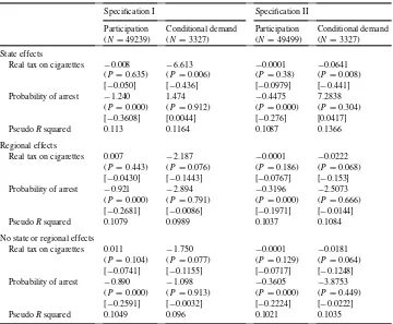
Table 2
Real tax on cigarettes −0.008 −6.613 −0.0001 −0.0641 (P=0.635) (P=0.006) (P=0.38) (P=0.008)
[−0.050] [−0.436] [−0.0979] [−0.441]
Probability of arrest −1.240 1.474 −0.4475 7.2838
(P=0.000) (P=0.912) (P=0.000) (P=0.304) [−0.3608] [0.0044] [−0.276] [0.0417]
PseudoRsquared 0.113 0.1164 0.1087 0.1366
Regional effects
Real tax on cigarettes 0.007 −2.187 −0.0001 −0.0222 (P=0.443) (P=0.076) (P=0.186) (P=0.068) [−0.0430] [−0.1443] [−0.0767] [−0.153] Probability of arrest −0.921 −2.894 −0.3196 −2.5073
(P=0.000) (P=0.791) (P=0.000) (P=0.666) [−0.2681] [−0.0086] [−0.1971] [−0.0144]
PseudoRsquared 0.1079 0.0989 0.1037 0.1084
No state or regional effects
Real tax on cigarettes 0.011 −1.750 −0.0001 −0.0181 (P=0.104) (P=0.077) (P=0.129) (P=0.064) [−0.0741] [−0.1155] [−0.0717] [−0.1248] Probability of arrest −0.890 −1.098 −0.3605 −3.8753
(P=0.000) (P=0.913) (P=0.000) (P=0.449) [−0.2591] [−0.0032] [−0.2224] [−0.0222]
PseudoRsquared 0.1049 0.096 0.1021 0.1035
aOwn- and cross-price/policy effects, NHSDA 1990–1996 marginal effect (P-value) [elasticity].
state fixed effect results suggest that marijuana and cigarettes are complements (the regional and no fixed effects models are discussed below). The cross-price effect for cigarettes in the marijuana participation and conditional demand models is negative, but statistically significant in only the conditional demand equation. Similarly, the probability of arrest, which can be thought of as a proxy for the price of marijuana in the absence of reliable price data, is negative and statistically significant in both parts of the two-part model for cigarettes for specification I (although small in magnitude, as one would expect).
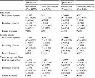
Table 3
Real tax on cigarettes −0.032 0.832 −0.0005 0.013 (P=0.269) (P=0.594) (P=0.116) (P=0.408) [−0.0866] [0.0519] [−0.128] [0.0768] Probability of arrest −0.582 −18.971 −0.4032 −1.7228
(P=0.000) (P=0.001) (P=0.000) (P=0.622) [−0.0712] [−0.0530] [−0.104] [−0.0095]
PseudoRsquared 0.1389 0.2031 0.1391 0.2106
Regional effects
Real tax on cigarettes −0.036 −0.990 −0.0005 −0.0127 (P=0.013) (P=0.205) (P=0.001) (P=0.101) [−0.0986] [−0.0617] [−0.140] [−0.0754] Probability of arrest −0.552 −19.298 −0.3234 −2.8578
(P=0.000) (P=0.000) (P=0.000) (P=0.33) [−0.0675] [−0.0539] [−0.0836] [−0.0158]
PseudoRsquared 0.1361 0.1918 0.1361 0.1953
No state or regional effects
Real tax on cigarettes −0.051 −1.014 −0.00071 −0.0132 (P=0.000) (P=0.105) (P=0.000) (P=0.035) [−0.1398] [−0.0632] [−0.1862] [−0.0783] Probability of arrest −0.532 −24.345 −0.2788 −4.4668
(P=0.000) (P=0.000) (P=0.000) (P=0.098) [−0.0650] [−0.0680] [−0.0721] [−0.0248]
PseudoRsquared 0.1346 0.1893 0.1345 0.1906
aOwn- and cross-price/policy effects, NHSDA 1990–1996 marginal effect (P-value) [elasticity].
With respect to cigarette demand, the own-price elasticities in both parts of the two-part model are imprecisely estimated (Table 3). Estimating cigarette demand for this age group is problematic during the 1990–1996 time period because the method to collect tobacco use among 12–17-year-old changed in 1994 from an interview format to a self-administered questionnaire (as was done for illicit drugs during the entire study period). Although we attempted to capture this effect with an indicator variable for the post-1993 period (and with price times the post-1993 indicator in another specification), we were not able to replicate standard price elasticities for youth. Based on recent estimates for this age group, one would expect total elasticities of demand from−0.4 to−0.6 (Evans and Huang, 1998; Farrelly and Bray, 1998; Tauras and Chaloupka, 1999).
Tables 2 and 3 also demonstrate the sensitivity of the estimates across various fixed effects models. Focusing first on the marijuana demand models, the effect of cigarette taxes on participation is statistically insignificant in all models. In specification I, the coefficient on taxes is negative in the state fixed effects models and becomes positive in the models with either regional or no fixed effects. In specification II, the result remains negative across the regional and no fixed effects specifications.
In contrast, the effect of cigarette taxes on conditional marijuana demand remains negative and statistically significant across all specifications, but the elasticity drops considerably as we move from the state to regional and no fixed effects models. This suggests that states with high levels of marijuana use have higher levels of cigarette taxation. The estimated effect for the probability of arrest remains relatively stable across all specifications.
In the cigarette demand models, the coefficient on taxes remains stable across all partic-ipation equations, while the standard error decreases from the state to regional to no fixed effects models, becoming statistically significant in the latter two models. However, in the conditional demand models, taxes remain imprecisely estimated in all specifications, with the exception of the no fixed effects model for specification II.
5.2. Gender differences
To further explore the effects of the probability of arrest and cigarette taxes on marijuana demand, we reestimate our models by gender (Table 4) using the probability of arrest defined for youth (specification I). These models reinforce the notion that marijuana and
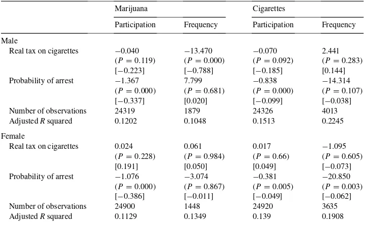
Table 4
Demand for cigarettes and marijuana by gendera
Marijuana Cigarettes
Participation Frequency Participation Frequency Male
Real tax on cigarettes −0.040 −13.470 −0.070 2.441
(P=0.119) (P=0.000) (P=0.092) (P=0.283)
[−0.223] [−0.788] [−0.185] [0.144]
Probability of arrest −1.367 7.799 −0.838 −14.314
(P=0.000) (P=0.681) (P=0.000) (P=0.107) [−0.337] [0.020] [−0.099] [−0.038]
Number of observations 24319 1879 24326 4013
AdjustedRsquared 0.1202 0.1048 0.1513 0.2245
Female
Real tax on cigarettes 0.024 0.061 0.017 −1.095
(P=0.228) (P=0.984) (P=0.66) (P=0.605)
[0.191] [0.050] [0.049] [−0.073]
Probability of arrest −1.076 −3.074 −0.381 −20.850
(P=0.000) (P=0.867) (P=0.005) (P=0.003) [−0.386] [−0.011] [−0.049] [−0.062]
Number of observations 24900 1448 24920 3635
AdjustedRsquared 0.1129 0.1349 0.139 0.1908
cigarettes are economic complements among males. For males, the effects of cigarette taxes on marijuana demand increase considerably relative to the results for the overall sample, while the effects for the probability of arrest remain stable. These results also show that the only result that remains robust for females is the deterrent effect of the probability of arrest on marijuana participation.
Turning to cigarette demand, the tax coefficient remains imprecisely estimated in all models with the exception of the participation model for males, where taxes are statistically significant at the 10% level and yield a reasonable price elasticity of roughly−0.2.
5.3. Marijuana possession laws
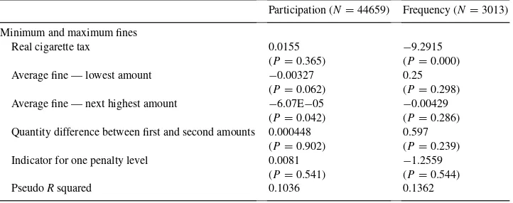
When deciding whether or not and how frequently to use marijuana, youths may also consider the penalties for marijuana possession in addition to the probability of arrest. As noted above, state marijuana laws generally take the form of a step function that is at the discretion of state legislators. To quantify the effect of these penalties on use, we reestimated our marijuana demand models including the average penalties (average of the minimum and maximum fines) for the first two steps in the penalty functions of states.3
Each step is characterized by the quantity interval (generally starting with any positive quantity up to 1 ounce and then from 1 to 4 ounces) and the penalty for possession of these amounts. Because a few states have one set of penalties for all possession violations, we also include an indicator variable for these states. Finally, because the height of this first step — or the difference in the penalty between the first and second quantity interval — varies from state to state, we also include the amount in grams required to trigger the second level of penalties. In theory, this variable is important because it captures the effect of more or less stringent penalty scales. One would expect, ceteris paribus, requiring greater quantities of marijuana to trigger a higher level of fine might encourage more and/or more frequent use. Table 5 shows that higher penalties for possession are correlated with a lower probability of use in the past 30 days. Both the average fine for the lowest quantity level and next highest quantity level are negative and statistically significant. However, higher fines do not appear to affect the frequency of marijuana use among young adults. The amount required to trigger a higher penalty level (the difference between the first and second amounts) had no effect on the probability of use.
Therefore, both a higher probability of arrest and higher fines decrease the probability of use, but not the frequency of use. Consistent with the results for the probability of arrest, higher penalties discourage the probability of marijuana use in the past 30 days but do not discourage the frequency of use. In addition, the effect of higher cigarette taxes on frequency of marijuana use remains robust in this alternative specification.
We also estimated the effects of these penalty variables in cigarette demand and, once again, confirmed a pattern of complementarity. However, none of the effects were statisti-cally significant (data not shown).
3We also estimated models including both the minimum and maximum fines, and although the results were
Table 5
Effects of marijuana possession fines on marijuana use, NHSDA 1990−1996
Participation (N=44659) Frequency (N=3013) Minimum and maximum fines
Real cigarette tax 0.0155 −9.2915
(P=0.365) (P=0.000)
Average fine — lowest amount −0.00327 0.25
(P=0.062) (P=0.298) Average fine — next highest amount −6.07E−05 −0.00429
(P=0.042) (P=0.286) Quantity difference between first and second amounts 0.000448 0.597
(P=0.902) (P=0.239)
Indicator for one penalty level 0.0081 −1.2559
(P=0.541) (P=0.544)
PseudoRsquared 0.1036 0.1362
6. Conclusion
Two clear policy implications emerge from the various models that we present in this paper. First, higher cigarette taxes decrease the intensity of marijuana use and may have a modest effect on the probability of use, especially among males. Overall, the total marijuana demand cross-price elasticity for cigarettes indicates that a 10% increase in cigarette prices would lead to a 5.4% decrease in total marijuana use (with a 95% confidence interval of 0–11%). We also found that these cross-price effects were driven by the males in the sample. For males, 10% increase in cigarette prices would lead to a 10% decrease in total marijuana demand (95% confidence interval of 3–19%). Therefore, although some have suggested that increases in cigarette prices may lead to an increase in marijuana use, the evidence presented in this paper suggests that these fears may be unfounded. All of the evidence in this paper supports that there is a complementary relationship between marijuana and cigarettes and that policies that are aimed at reducing cigarette use are likely to also reduce marijuana use. Second, both higher fines for marijuana possession and increased probability of arrest decrease the probability that a young adult will use marijuana, but these policies have little effect on the frequency of use.
Acknowledgements
This work was supported by a grant from the National Institutes on Drug Abuse (Da11297) and the Substance Abuse and Mental Health Services Administration under contract number 283-93-5409. The authors would like to thank Rosalie Pacula for helpful comments, Andrew Sfekas for excellent research assistance, and Joanne Kempen and Susan Murchie for editorial assistance.
Appendix A
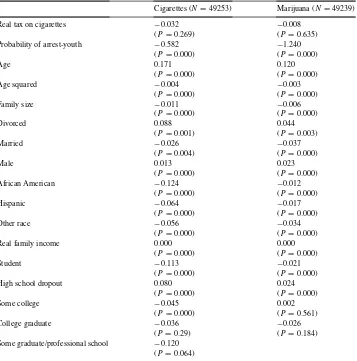
The full models are presented in Table 6
Table 6
Basic participation model with own– and cross–price/policy effects for youthsa
Cigarettes (N=49253) Marijuana (N=49239)
Real tax on cigarettes −0.032 −0.008
(P=0.269) (P=0.635)
Probability of arrest-youth −0.582 −1.240
(P=0.000) (P=0.000)
Age 0.171 0.120
(P=0.000) (P=0.000)
Age squared −0.004 −0.003
(P=0.000) (P=0.000)
Family size −0.011 −0.006
(P=0.000) (P=0.000)
Divorced 0.088 0.044
(P=0.001) (P=0.003)
Married −0.026 −0.037
(P=0.004) (P=0.000)
Male 0.013 0.023
(P=0.000) (P=0.000)
African American −0.124 −0.012
(P=0.000) (P=0.000)
Hispanic −0.064 −0.017
(P=0.000) (P=0.000)
Other race −0.056 −0.034
(P=0.000) (P=0.000)
Real family income 0.000 0.000
(P=0.000) (P=0.000)
Student −0.113 −0.021
(P=0.000) (P=0.000)
High school dropout 0.080 0.024
(P=0.000) (P=0.000)
Some college −0.045 0.002
(P=0.000) (P=0.561)
College graduate −0.036 −0.026
(P=0.29) (P=0.184) Some graduate/professional school −0.120
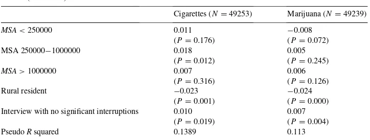
Table 6 (Continued)
Cigarettes (N=49253) Marijuana (N=49239)
MSA<250000 0.011 −0.008 Interview with no significant interruptions 0.010 0.007
(P=0.019) (P=0.004)
PseudoRsquared 0.1389 0.113
aAlso included but not shown: state and year effects, and a dummy variable for year >1994.
.
References
Benson, B.L., Rasmussen, D.W., 1991. Relationship between illicit drug enforcement policy and property crimes. Contemporary Policy Issues IX, 106–115.
Benson, B.L., Kim, I., Rasmussen, D.W., Zuehlke, T.W., 1992. Is property crime caused by drug use or by drug enforcement policy? Appl. Econ. 24, 679–692.
Chaloupka, F.J., Laixuthai, A., 1997. Do youths substitute alcohol for marijuana? Some econometric evidence. Eastern Econ. J. 23 (3), 253–276.
Chaloupka, F.J., Pacula, R.L., Farrelly, M.C., Johnston, L.D., O’Malley, P.M., Bray, J.W., 1999. Do higher cigarette prices encourage youth to use marijuana? Working paper.
DiNardo, J., Lemieux, T., 1992. Alcohol, marijuana, and American youth: the unintended effects of government regulation. National Bureau of Economic Research, Working paper 4122.
Duncan, S.C., Duncan, T.E., Hops, H., 1998. Progressions of alcohol, cigarette, and marijuana use in adolescence. J. Behav. Med. 21 (4), 375–388.
Ellickson, P.L., Hays, R.D., Bell, R.M., 1992. Stepping through the drug use sequence: longitudinal scalogram analysis of initiation and regular use. J. Abnormal Psychol. 101, 441–451.
Evans, W.N., Huang, L.X., 1998. Cigarette taxes and teen smoking: new evidence from panels of repeated cross-sections. University of Maryland, Department of Economics, Working paper.
Farrelly, M.C., Bray, J.W., 1998. Response to increases in cigarette prices by race/ethnicity, income, and age groups — United States, 1976–1993. Centers for Disease Control and Prevention (CDC), Morbidity and Mortality Weekly Report 47 (29), 605–609.
Hoyt, G.M., Chaloupka, F.J., 1993. Self-reported substance use and survey conditions: an examination of the National Longitudinal Survey of Youth. In: Presented at the Western Economic Association Annual Meeting, Lake Tahoe, June 23.
Kandel, D., 1975. Stages in adolescent involvement in drug use. Science 190, 912–914.
Kandel, D., Faust, R., 1975. Sequence and stages in patterns of adolescent drug use. Arch. Gen. Psychiatry 32, 923–932.
Kandel, D.B., Yamaguchi, K., 1993. From beer to crack: developmental patterns of drug involvement. Am. J. Public Health 83 (6), 851–855.
Kelly, T.H., Foltin, R.W., Rose, A.J., Fischman, M.W., Brady, J.V., 1990. Smoked marijuana effects on tobacco cigarette smoking behavior. J. Pharmacol. Exp. Therapeutics 252 (3), 934–944.
Model, K., 1993. The effect of marijuana decriminalization on hospital emergency drug episodes: 1975–1978. J. Am. Stat. Assoc. 88, 423.
Pacula, R.L., 1998a. Does increasing the beer tax reduce marijuana consumption? J. Health Econ. 17 (5), 557–585. Pacula, R.L., 1998b. Adolescent alcohol and marijuana consumption: is there really a gateway effect? National
Bureau of Economic Research, Working paper 6348.
Rasmussen, D.W., Benson, B.L., 1994. The Economic Anatomy of a Drug War: Criminal Justice in the Commons. Rowman & Littlefield, Lanham, MD.
Saffer, F., Chaloupka, F.J., 1998. Demographic differentials in the demand for alcohol and illicit drugs. National Bureau of Economic Research, Working paper 6432.
Simmons, M.S., Tashkin, D.P., 1995. The relationship of tobacco and marijuana smoking characteristics. Life Sci. 56 (24), 2185–2191.
Substance Abuse and Mental Health Services Administration (SAMHSA), 1992. National Household Survey on Drug Abuse: Public Release Codebook 1991. US Department of Health and Human Services, Rockville, MD. Substance Abuse and Mental Health Services Administration (SAMHSA), 1994. National Household Survey on Drug Abuse: Public Release Codebook 1992. US Department of Health and Human Services, Rockville, MD. Substance Abuse and Mental Health Services Administration (SAMHSA), 1996. The development and implementation of a new data collection instrument for the 1994 National Household Survey on Drug Abuse. US Department of Health and Human Services, Rockville, MD.
Substance Abuse and Mental Health Services Association (SAMHSA), 1998. Preliminary results from the 1997 National Household Survey on Drug Abuse: fact sheet. US Department of Health and Human Services, Rockville, MD.
Tauras, J.A., Chaloupka, F.J., 1999. Price, clean indoor air laws, and cigarette smoking: evidence from longitudinal data for young adults. National Bureau of Economic Research, Working paper 6937.
Thies, C.F., Register, C.A., 1993. Decriminalization of marijuana and the demand for alcohol, marijuana, and cocaine. Social Sci. J. 30 (4), 385–399.
Tobacco Institute, 1997. The Tax Burden on Tobacco: Historical Compilation 1993, Vol. 28. Tobacco Institute, Washington, DC.
Turner, C., Lessler, J., Devore, J., 1992. Effects of mode of administration and wording on reporting of drug use. Survey Measurement of Drug Use: Methodological Studies. National Institute on Drug Abuse, Rockville, MD. Yamaguchi, K., Kandel, D.B., 1984. Patterns of drug use from adolescence to young adulthood. III. Predictors of