Drawing 3-Polytopes with Good Vertex
Resolution
Andr´
e Schulz
Institut f¨ur Mathematsche Logik und Grundlagenforschung, Universit¨at M¨unster
Abstract
We study the problem how to obtain a small drawing of a 3-polytope with Euclidean distance between any two points at least 1. The problem can be reduced to a one-dimensional problem, since it is sufficient to guarantee distinct integer x-coordinates. We develop an algorithm that yields an embedding with the desired property such that the polytope is contained inside a 2(n−2)×2×1 box. The constructed embedding
can be scaled to a grid embedding whose x-coordinates are contained in [0,2(n−2)]. Furthermore, the point set of the embedding has a small
spread, which differs from the best possible spread only by a multiplicative constant.
Submitted:
December 2009
Reviewed:
September 2010
Revised:
October 2010
Accepted:
November 2010
Final:
November 2010
Published:
February 2011
Communicated by:
D. Eppstein and E. R. Gansner
Article type:
Regular paper
Supported by the German Research Foundation (DFG) under grant SCHU 2458/1-1.
1
Introduction
Let G be a 3-connected planar graph with n vertices v1, . . . , vn and edge set
E. A 3-polytope is a polytope in 3d with full dimension. The face lattice of a 3-polytope is entirely determined by its edge graph. Due to Steinitz’ seminal theorem [19] we know that G admits a realization as the edge graph of a 3-polytope, and every edge graph of a 3-polytope is planar and 3-connected. The question arises how one can obtain a “nice” realization of a 3-polytope when its graph is given. One particular property, which is often desired from an aesthetically point of view, is that the vertices of the embedding should be evenly distributed. If two vertices lie too close together they are hard to distinguish. Such an embedding may appear as bad “illustration” for the human eye. Of course we can always scale a 3-polytope to increase all of its pointwise distances, but this does not affect the relative distances and the subjective perception of the viewer stays the same. Therefore, we restrict ourselves to an embedding whose vertices have, pairwise, an Euclidean distance of at least 1. We say that in this case the embedding/drawing is under the vertex resolution rule. See [2] for a short discussion on resolution rules. Resolution rules depend on a particular distance measure. Throughout the paper we use the Euclidean distance, but our results can be easily modified for other distance measures such asL1orL∞.
In 2d, drawings of planar graphs can be realized on anO(n)×O(n) grid [6, 16]. Since the grid is small, these grid embeddings give a good vertex resolution for free. The situation for 3-polytopes is different. The best known algorithm uses a grid of sizeO(27.21n) [1, 14]. Thus, the induced resolution might be bad
for this embedding.
Let us briefly discuss some approaches for realizingGas 3-polytope. Steinitz’ original proof is based on a transformation ofGto the graph of the tetrahedron. The transformation consists of a sequence of local modifications that preserve the realizability of G as 3-polytope. The Koebe-Andreev-Thurston Theorem on circle packings gives another proof of Steinitz’ Theorem (see for example Schramm [17]). This approach relies on non-linear methods which makes many geometric features of the constructed 3-polytope intractable. A third approach uses liftings of planar graphs with equilibrium stress (known as the Maxwell-Cremona correspondence [22]). In order to construct a plane embedding with equilibrium stress the intermediate 2d drawing is obtained as barycentric em-bedding by the method of Tutte [20, 21]. This powerful approach is used in a series of embedding algorithms: Eades and Garvan [7], Richter-Gebert [15], Chrobak, Goodrich, and Tamassia [2], Rib´o Mor, Rote, and Schulz [14]. We refer to this approach as lifting approach. A completely different approach is due to Das and Goodrich [5]. It uses an incremental technique which only needs O(n) arithmetic operations for embedding Gas 3-polytope, but works only for triangulated planar graphs.
show how to compute a barycentric embedding and how to apply the Maxwell-Cremona correspondence. This part contains well-known concepts. In general it is not possible to lift a barycentric embedding. The applicability of the Maxwell– Cremona correspondence depends on the selected boundary. Thus we have to select the location of the boundary such that the 2d drawing is liftable. This can be achieved by the methods presented in [14]. For completeness we discuss this part in Section 3. Since we are interested in a 2d embedding that will give a good vertex resolution in the lifting we have to find a way to control the 2d embedding (presented in Section 4). This will be done by adjusting the barycentric weights that specify the 2d drawing. It suffices to guarantee small distinct integer x-coordinates to assure the vertex resolution rule. We follow the construction of [2] to guarantee distinctx-coordinates. In order to find an appropriate location of the boundary face we have to find a way tocontrol the barycentric weights even further. These tools are crucial for the design of the algorithm and are developed in Section 4. After presenting the embedding algo-rithm in Section 5 we present additional properties of the computed embeddings in Section 6 and conclude with an example in Section 7.
Results: We show how to obtain an embedding of Gas 3-polytope inside a 2(n−2)×2×1 box under the vertex resolution rule. It is even possible to make the box arbitrarily flat such that its volume gets arbitrarily small. But for aesthetic reasons we leave the side lengths at least 1. Our algorithm follows the lifting approach and extends the ideas of [14]. In contrast to the construction of [14] we use more complicated interior edge weights. Our algorithm creates an embedding with two more interesting properties: (1) it can be scaled to a grid embedding whosex-coordinates are in [0,2(n−2)], and (2) the point set of the embedding has a good ratio between its largest and shortest pointwise distance. We show that this number differs only by a constant from the best possible ratio.
have to make use of the new techniques developed in Lemma 4 and 5.
2
Preliminaries: Maxwell and Tutte
In this section we review Tutte’s barycentric 2d embeddings and the Maxwell-Cremona correspondence. Both tools are well established necessary ingredients for the lifting approach.
Since G is 3-connected and planar, the facial structure of G is uniquely determined [23]. Let us pick an arbitrary face fb, which we call the boundary
face. We assume further that the vertices are ordered such that v1, v2, . . . , vk
are the vertices of fb in cyclic order. An edge (vertex) is called a boundary
edge (vertex) if it lies onfb, otherwise it is called aninterior edge (vertex). In
this paper every embedding is considered as plane straight-line embedding. A 2d embedding ofGis specified by giving every vertexvia coordinatepi= (xi, yi)T.
We denote the 2d embedding asG(p) and consider only embeddings that realize fb as a convex outer face.
To describe the Maxwell-Cremona correspondence we introduce the concept ofequilibrium stresses.
Definition 1 (Stress, Equilibrium) An assignmentω:E →Rof scalars to the edges of G (with ω(i, j) =:ωij=ωji) is called a stress. Let G(p) be a 2d
embedding ofG. A pointpi is in equilibrium if and only if
X
j:(i,j)∈E
ωij(pi−pj) = 0. (1)
The embedding of G is in equilibrium if and only if all of its points are in equilibrium.
IfG(p) is in equilibrium according to ω, thenω is called an equilibrium stress
forG(p). Of special interest are stresses that are positive on every interior edge ofG. These stresses are calledpositive stresses.
Suppose we fix an embeddingG(p) in the plane. Leth: V →Rbe a height assignment for the vertices ofG. The functionhdefines a 3d embedding ofG by giving every vertexpi the additionalz-coordinatezi =h(pi). If in the 3d
embedding every face ofGlies on a plane the height assignment his called a
lifting. The Maxwell-Cremona correspondence describes the following.
Theorem 1 (Maxwell [12], Whiteley [22]) Let G be a 3-connected planar graph with 2d embedding G(p) and a designated face fˆ. There exists an 1-1 correspondence between
A.) equilibrium stressesω onG(p),
The complete proof of the Maxwell-Cremona correspondence is due to White-ley [22] (see also [4]). Richter-Gebert’s book [15, Section 13] contains a simple algorithm that computes the lifting: The location of every face in the lifting is specified byG(p) and a plane on which the face lies. For convenience we intro-duce for every vertexpi= (xi, yi)T a (homogenized) 3d vertexp′i := (xi, yi,1)T.
We define for every facefj a vector qj ∈R3, such that hqj,pi describes the
height of the point p ∈ fj in the lifting. The vectors qj can be computed
incrementally by
qb= (0,0,0)T,
ql=ωij(pi′×p′j) +qr,
(2)
where the edge pointing fromi toj separates the faces fl andfr, such thatfl
lies to the left and fr lies to the right. Notice that the computed lifting does
not depend on the order of the faces that is used to determine theqvectors. To apply the Maxwell-Cremona correspondence one needs a 2d embedding ofGwith equilibrium stress. Barycentric embeddings can generate drawings for which the equilibrium condition (1) holds for all interior vertices. Letω be an arbitrary stress that is positive on the interior edges and zero on the boundary edges. (It is valid to select stresses of value 0 on the boundary because the boundary stress weights do not affect the barycentric embedding.) We obtain from the stressω itsLaplace matrix L={lij}, which is defined by its entries as
lij :=
−ωij if (i, j)∈Eand i6=j, P
jωij ifi=j,
0 otherwise.
An embedding G(p) is described by the vectors x = (x1, . . . , xn)T and y =
(y1, . . . , yn)T. Let B :={1, . . . , k} andI :={k+ 1, . . . , n} be the index sets of
the boundary and interior vertices, respectively. We subdividex,y, and Lby B and I and obtain xB,xI,yB,yI, LBB, LII, LBI and LIB. The equilibrium
condition (1) for the interior vertices can be phrased asLIBxB+LIIxI =0.
The same holds for the y-coordinates. This implies that we can express the vectorsxI andyI as linear functions in terms of xB andyB, namely by
xI =−L−II1LIBxB, yI =−L−II1LIByB. (3)
The matrixLII is singular and hence the vectors xI andyI are properly and
uniquely defined (see [15, 8]). The embedding is known as the (weighted) barycentric embedding. For every positive stress and convex boundary face the coordinates give a strictly convex straight-line embedding (see for example [8]). A weighted barycentric embedding has the following nice interpretation: The interior edges of the graph can be considered as springs with spring constants ωij. The barycentric embedding models the equilibrium state of the system of
3
Extending an Equilibrium Stress to the
Bound-ary
The interior vertices computed by (3) are in equilibrium by construction. How-ever, the stressed edges of the boundary vertices do not sum up to zero, but to
∀i∈B X
j:(i,j)∈E
ωij(pi−pj) =:Fi. (4)
To apply the Maxwell-Cremona correspondence we have to alter the stress on the boundary edges (which we set to 0) such that it cancels the vectorsFi.
Adjust-ing the stress weights on the boundary does not interfere with the barycentric embedding. If the outer face is a triangle it is always possible to cancel the
Fi vectors by solving a linear system with three unknowns [9]. But in general
this is only possible for special locations of the boundary face. We use the method of Rib´o Mor, Rote, and Schulz [14] to extend the equilibrium stress to the boundary.
Lemma 1 (Substitution Lemma [14]) There are weightsω˜ij = ˜ωji, fori, j∈
B, independent of location of the boundary face such that
∀i∈B Fi= X
j∈B:j6=i
˜
ωij(pi−pj). (5)
The weights ω˜ij are the off-diagonal entries of −LBB+LBIL−II1LIB, which is
the Schur Complement ofLII inL multiplied with−1.
The proof of the Substitution Lemma can be found in [14]. The ˜ωvalues are independent of the location of the boundary face and depend only on the stress ω. From this point of view we can use the complete graphKk on the boundary
vertices with stress ˜ω as substitution for the embedding G(p) with stressω to express the vectorsFi. For this reason we call the stress ˜ωthesubstitution stress.
The different weights ˜ωij are named substitution stress entries. With help of
the substitution stress we can simplify the problem of locating the boundary face. A feasible location offb can be found by solving the non-linear system
consisting of the 2k equations of (5) (kequations for the x-coordinates, andk equations for they-coordinates) plus the 2kequations
∀i∈B:ωi,suc(i)(pi−psuc(i)) +ωi,pre(i)(pi−ppre(i)) =−Fi, (6)
wheresuc(i) denotes the successor of vi and pre(i) denotes the predecessor of
vionfb in cyclic order. Since the equations are dependent the system is
under-constrained. Later, we will fix some boundary coordinates to obtain a unique solution. An important property of the substitution stress entries was observed in [14].
Lemma 2 (Lemma 3.3(1) in [14]) If the stress ω is positive, then for every
i, j∈B the induced substitution stressω˜ij is positive.
4
Constructing and Controlling an
x
-Equilibrium
Stress
So far we followed the ideas of [14] and showed how to construct an embedding with equilibrium stress by using a barycentric embedding whose position of the outer face was computed in advance by a non-linear system. In order to use a barycentric embedding properly one has to show that the pre-computed outer face forms a convex polygon. This is only possible by deriving structural properties for the substitution stress. In addition to the construction of [14] we have to show that the vertex resolution rule holds. We explain in this section how to modify the barycentric weights, such that a set of prescribed x-coordinates are the solution of the barycentric embedding. Moreover we show how to update the barycentric weights further, such that one or two substitution stress entries become dominant while preserving thex-coordinates. Our goal is to select small distinct integer values for thex-coordinates, which would imply the vertex resolution rule. The structural property of the dominating stress entries will be later useful if we have to show that the boundary face is realized as convex polygon.
Let x1, . . . , xn now be the prescribed x-coordinates we want to achieve in
G(p). We are interested in a positive equilibrium stress that yields these x-coordinates in the barycentric embedding. In particular, we are looking for a positive stressω such that
∀i∈I X
j:(i,j)∈E
ωij(xi−xj) = 0. (7)
We call a positive stress that fulfills condition (7) a (positive) x-equilibrium stress. Since we consider in this paper only positive x-equilibrium stresses we omit the term “positive” in the following. A simple directed pathπ=vi1, vi2, . . . in G is called x-monotone if for all its vertices vik we have xik < xik+1. As pointed out in [2], anx-equilibrium stress exists if every interior edge lies on somex-monotone path, whose endpoints are boundary vertices. Let us assume that we have selected thex-coordinates such that the latter holds. Furthermore, let us pick for every edgeesome x-monotone pathPe.
We follow the approach of [2] to construct an x-equilibrium stress. The construction is based on assigning a costc{i,j} >0 to every interior edge (i, j)
ofG. If the costs guarantee ∀i∈I X
j:(i,j)∈E:xi<xj
c{i,j}=
X
(i,k)∈E:xi>xk
c{i,k}, (8)
we can define anx-equilibrium stress by setting ωij=
c{i,j}
|xi−xj|
. (9)
The costsc{i,j} can be constructed by the following incremental construction.
an edge with c{i,j} = 0. We increase the costs of the edges of Pe by 1. In
(8) both sides of the equation increase by 1 ifvi lies on Pe, otherwise nothing
changes. Hence, (8) still holds. We repeat this procedure until every interior edge is assigned with a positive cost. Since we have at most 3n−3 interior edges, the total cost for an edge is an integer smaller than 3n−3.
We show now how to modify anx-equilibrium stress to obtain helpful proper-ties for the substitution stress induced byω. Our goal is to obtain a substitution stress that realizes its maximal entry on an edge that we picked. More formally, letvsandvtbe two non-adjacent vertices on the boundary ofGand letα >1 be
a parameter that we pick later. The stressω should guarantee that for all pairs of boundary verticesvi,vj we have ˜ωst > α˜ωij, unless{i, j}={s, t}. Our idea
for how to achieve this is the following: We pick anx-monotone pathPst from
vs to vt. Then we determine a suitable (large) number K, and add K to the
costs of every edge which is onPst. The stress induced by the increased costs
is still an x-equilibrium stress for our choice of x-coordinates. If we think of the stresses as spring constants, we have increased the force that pushesvsand
vt away from each other. Our hope is that this will reflect in the substitution
stress and make ˜ωst the dominant stress entry.
First, let us bound the substitution stress on all edges from above and then prove a lower bound for the stress ˜ωst.
Lemma 3 LetL={lij} be the Laplace matrix derived from a positive stressω,
andω˜ the corresponding substitution stress. For anyi, j∈B we have
˜
ωij<min{lii, ljj}.
Proof: Since uTLu = P
(i,j)∈Eωij(ui −uj)2, which is non-negative for any
vectoru, the Laplace matrix is positive semidefinite. Let ˜L ={˜lij} =LBB−
LBIL−II1LIB denote the Schur complement of LII in L. Due to [24, page 175]
LII−L˜is positive semidefinite. Therefore, all principal submatrices are positive
semidefinite and we havelii≥˜lii. As a consequence of the substitution lemma,
we know thatP
j∈B:i6=jω˜ij = ˜lii, and hence Pj∈B:i6=jω˜ij ≤lii. Since each of
the ˜ωij’s is positive, each summand has to be smaller than lii. By the same
argument ˜ωij ≤ljj, which proves the lemma.
The next lemma proves a lower bound for ˜ωst and determines the numberK
that guarantees that ˜ωst becomes the dominant stress.
Lemma 4 Letω be anx-equilibrium stress obtained from the edge costsc{i,j}<
3n forx1, . . . , xn that is increased along an x-monotone path from vs tovt, by
incrementing the edge costs for edges on the path byK. The substitution stress and the matrixL are obtained fromω as usual. Then
˜ ωst>
K−3n2(1 + (k−2)∆
x)
xt−xs
,
where k denotes the number of boundary vertices and ∆x the largest distance
between twox-coordinates. For anyα >0we can pickK≥3n2(1+(α+k−2)∆
and obtain for anyω˜ij that is notω˜st
˜
ωst> αω˜ij.
Proof:Before bounding ˜ωstwe show an upper bound for the other substitution
stress entries. Let (i, j) an edge that is not (s, t). By Lemma 3, ˜ωij is less than
lrr (r ∈ {i, j} \ {s, t}). Since lrr is a diagonal entry of the Laplace matrix it
equals P
u:(r,u)∈Eωru, which is a sum of at most n−1 summands. We can
assume that the pathPst uses no boundary edge. In this case each summand
inP
t be thex-component ofFt. We combine (10) and (5) and obtain as upper
bound forFx t
˜
ωst(xt−xs) + (k−2)3n2∆x> Ftx.
On the other hand we can expressFx
t by (4). The cost of one edge (w, t), with
Combining the two bounds for Fx
t leads to the bound for ˜ωst as stated in the
As the last part of this section we show that we can even enforce a pair of substitution stress entries to be dominant if we have at least 5 vertices on the boundary face. Letvt1, vt2 be two vertices that are both non-adjacent tovsand letxt1 =xt2. We can increment a givenx-equilibrium stress by first increasing the edge costsc{i,j} along an x-monotone path from vs to vt1 byK and then do the same for an appropriate path fromvs tovt2.
Lemma 5 Assume the same as in Lemma 4, but this time consider two paths: from vs to vt1 and from vs to vt2. Assume further that xt1 = xt2. For K ≥ 3n2(1 + (α+k−2)∆x)we have for anyω˜ij with {i, j} 6⊂ {s, t1, t2}
˜
ωst1 > αω˜ij, and ω˜st2 > α˜ωij.
Proof:Lemma 4 relies on the fact that we can boundP
j6=sω˜jt(xt−xj) because
by (10) the ˜ω′s in this sum are small. We cannot use this bound for ˜ω
steps of the proof of Lemma 4 with first choosing t = t1 and then choosing
t=t2 proves the lemma.
Notice that the bounds for K are very rough. Better bounds can be easily obtained, but they result in more complicated expressions. Since for our purpose the fact that we can always find a valid numberKis more important than the smallest possible size ofK, we presented a simple bound forK.
5
The Embedding Algorithm
5.1
The Algorithm Template
In this section we present as the main result of this paper
Theorem 2 Let Gbe a 3-connected planar graph. Gadmits an embedding as 3-polytope inside a2(n−2)×2×1 box under the vertex resolution rule.
We prove Theorem 2 in the remainder of this section by introducing an algorithm that constructs the desired embedding. The number of vertices on the boundary face plays an important role. The smaller this number is, the simpler is it to construct an embedding. For this reason we choose as boundary face fb the
smallest face ofG. Due to Euler’s formulafbhas at most 5 vertices. Depending
on the size offb we obtain three versions of the algorithm which all follow the
same basic pattern.
Our goal is to construct a planar embedding ofGthat has a positive stress and whosex-coordinates are distinct integers. The corresponding lifting of such an embedding fulfills the vertex resolution rule independently of its y and z-coordinates. Hence, we can scale in the direction of they and z-axis without violating the vertex resolution rule. The basic procedure is summarized in Algorithm 1.
Algorithm 1:Embedding algorithm as template.
1: Choose thex-coordinates.
2: Construct anx-equilibrium stressω.
3: Choose the boundaryy-coordinates.
4: EmbedGas barycentric embedding with stressω and the selected boundary in the plane.
5: Lift the plane embedding.
Step 1: The selection of the x-coordinates for G(p) is independent of the size of fb. We start with some strictly convex plane embedding of G – called
a pre-embedding. Let ˆx1, . . . ,xˆn and ˆy1, . . . ,yˆn be the coordinates of the
The actual values of these coordinates depend on the size offb, and are given
in Section 5.2–5.4. We assume that in the pre-embedding allx-coordinates are different. If this is not the case we can perturb the stress of the (pre)-embedding to achieve this. Since the pre-embedding is strictly convex [21] every edge lies on somex-monotone path. As it was done in Section 4, we fix for every interior edgeesuch a pathPe. Thex-coordinates of the pre-embedding induce a strict
linear order on the vertices ofG. We denote withbi the number of vertices with
smaller ˆx-coordinate compared to ˆxiin the pre-embedding. Thex-coordinates of
the (final) embedding are defined asxi:=bi. Thus, no two vertices get the same
x-coordinate and the largest x-coordinate is less thann. The paths Peremain
x-monotone in G(p). Therefore, they can be used to define an appropriate x-equilibrium stress ω. For technical reasons we might choose the same x-coordinate for some of the boundary vertices. In this case we check the vertex resolution rule for these vertex pairs inG(p) separately.
Steps 2 and 3: These steps are the difficult part of the algorithm. We have to choose the stressω and the boundary y-coordinates such that an extension of the stress to the boundary is possible. Moreover, the boundary coordinates have to yield a convex boundary face. After computing ω we can derive the substitution stress. The feasible location of the boundaryy coordinates is then expressed in terms of the substitution stress entries. We explain steps 2 and 3 in Section 5.2, 5.3 and 5.4 for the three different cases separately. To execute step 2 we have to apply the techniques developed in Section 3 and 4.
Steps 4 and 5: This part is a straightforward application of the barycentric embedding and the Maxwell-Cremona correspondence (see Section 2). The value of the (extended) stress on the boundary edges is not needed to compute the lifting, because we can place an interior face in thexy-plane and then compute the lifting using only interior edges.
5.2
Graphs with Triangular Face
The case wherefb is a triangle is the easiest case because we can extend every
stress to the boundary for every location of the outer face (see Section 3). This case was already addressed by Chrobak, Goodrich and Tamassia [2]. The discussion in this section will prove the following statement:
Proposition 1 LetGbe a3-connected planar graph and letGcontain a trian-gular face. G admits an embedding as 3-polytope inside an(n−1)×1×1 box under the vertex resolution rule.
Proof:Let us compute the pre-embedding with the boundary coordinates ˆx1= 0,x2ˆ = 1,and ˆx3= 0. We use thex-monotone pathsPeto compute a suitable
x-equilibrium stressωas discussed in Section 4. Next we compute the barycentric embedding forωwith boundary coordinatesp1= (0,0)T,p2= (n−1,0)T,and
Any two vertices have distance at least 1, since theirx-coordinates differ by at least 1. (This is not true forv1 andv3, but their distance isy3−y1= 1.)
5.3
Graphs with Quadrilateral Face
Let us now assume thatGcontains a quadrilateral but no triangular face. In this case it is not always possible to extend an equilibrium stressωto the boundary. The observations of Section 3 help us to overcome this difficulty.
Proposition 2 LetGbe a3-connected planar graph and letGcontain a quadri-lateral face. Gadmits an embedding as 3-polytope inside a2(n−2)×1×1 box under the vertex resolution rule.
Proof: We use as boundary coordinates for the pre-embedding ˆx1 = 0,x2ˆ = 1,x3ˆ = 1, and ˆx4 = 0. Thex-coordinates induced by the pre-embedding give x2 = x3 = n−2. We redefine the boundary x-coordinates by setting x3 = 2(n−2). This maintains the x-monotonicity of the paths Pe, but makes it
easier to extend the stress to the boundary as we will see in the following. Let ω be the x-equilibrium stress for the selected x-coordinates. For the later analysis it is helpful to have a “dominant” substitution stress entry. We therefore modifyω with the technique described in Section 4. After increasing the costs along anx-monotone path π from v1 to v3 by 18n3 we can assume that ˜ω13 > ω24. This follows from the application of Lemma 4 with˜ α = 1, ∆x= 2(n−2), andk= 4. For these values 18n3>3n2(1 + (α+k−2)∆x) and
thus the increment of the costs alongπsuffices.
Let us now discuss how to extend the stress ω to the boundary. To solve the non-linear system given by (5) and (6) we fix some of the boundary y-coordinates to obtain a unique solution. In particular, we sety1 = 0, y2 = 0, andy4= 1. As final coordinate we obtain1
y3= ω24˜ 2˜ω13−ω24˜ .
Since ˜ω13 >ω24, we can deduce that 0˜ < y3 <1. Hence, all y-coordinates are contained in [0,1]. Furthermore, we know that the only two vertices with the samex-coordinate, namelyv1 andv4, have the distance y4−y1= 1. Therefore the vertex resolution rule holds. Finally, we scale the induced lifting such that
the largestz-coordinate equals 1.
5.4
The general case
Proof of Theorem 2. To prove the theorem we can assume that the boundary face contains 5 vertices. The other cases were already covered by Proposition 1 and 2. This however is the most complicated case. We follow the construction of the proof of Proposition 2 and compute a pre-embedding. We choose as the x-coordinates for the pre-embedding of the outer face ˆx1= 0,x2ˆ = 1,x3ˆ = 1,x4ˆ =
0, and ˆx5=−ε, forε >0 small enough to guarantee that all interior vertices get a positive ˆx-coordinate in the pre-embedding. The pre-embedding induces the desiredx-coordinates forG(p) (step 1 of Algorithm 1). We change the induced x-coordinates on the boundary without changing the “monotonicity” of the pathsPe by settingx1= 0, x2=n−2, x3=n−2, x4= 0, andx5=−(n−2).
For the later analysis it is helpful to have two “dominating” substitution stress entries. This can be achieved with the method introduced in Section 4: We increase the costs, that defineω along anx-monotone path fromv5 to v2, and along anx-monotone path fromv5 tov3. The increment is in both cases 36n3. The application of Lemma 5 withα= 3, k= 5, and ∆x= 2(n−2) yields
˜
ω25>3˜ω13,ω25˜ >3˜ω14,ω25˜ >3˜ω24,ω35˜ >3˜ω13,ω35˜ >3˜ω14,ω35˜ >3˜ω24, (11) since 36n2>3n2(1+(α+k−2)∆
x). We can apply the lemma, becausex2=x3.
Appropriate boundary y-coordinates can be obtained by solving the non-linear system given by (5) and (6). As in the proof of Proposition 2 we fix some y-coordinates to obtain a unique solution. We sety1=−1, y4= 1, andy5= 0. This yields the two remainingy-coordinates
y2 = −2−2ω24˜˜ ω13−ω˜
Two things need to be checked for the solution fory2 andy3: (1) fb has to be
convex and (2)y3−y2has to be large enough to guarantee the vertex resolution rule. First we show that−2 < y2 and y3 <2, which would imply that fb is
Both inequalities are true, because as a consequence of (11) the only positive summand ˜ω24ω13˜ is smaller than ˜ω35ω13˜ and smaller than ˜ω25ω24. The difference˜ and hence the fraction is greater−1.
We finish this section with some remarks on the running time of the embed-ding algorithm. As mentioned in [2] thex-equilibrium stress can be computed in linear time. The barycentric embedding (which we use twice, once for the pre-embedding and once for the intermediate plane embedding) can be com-puted by the linear system (3). Since the linear system is based on a planar structure, it can be solved with nested dissections (see [10, 11]) based on the planar separator theorem. As a consequence a solution can be computed in O(M(√n)) time, whereM(n) is the upper bound for multiplying twon×n ma-trices. The current record forM(n) is O(n2.325), which is due to Coppersmith and Winograd [3]. The computation of the lifting can be done in linear time. In total, we achieve a running time ofO(n1.1625).
6
Additional Properties of the Embedding
6.1
Induced Grid Embedding
In addition to the small embedding under the vertex resolution rule, the con-structed embedding has several other nice properties which we discuss in this section. Since the computedy andz-coordinates are expressed by a linear sys-tem of rational numbers, they are rational numbers as well. Thus, we can scale the final embedding to obtain a grid embedding. We first prove a technical lemma.
Lemma 6 Suppose that all x and y-coordinates as well as the stress ω are integral. Let the difference between two x-coordinates be less than ∆x and let
the difference between twoy-coordinates be less than∆y. Then the height zi of
any pointpi in the lifting is an integer and it can be bounded by
0≤zi≤ |ω12| ·∆x·∆y,
whereω12 is a stress on an arbitrary boundary edge.
Proof:Since by (2) all heights can be expressed as additions and multiplications of integers, the heights are integral. Moreover, all heights are invariant under rigid motions of the plane embedding. Hence, we can assume thaty1=y2= 0, x1= 0, and ally-coordinates are non-negative. The lifted polytope lies between the planes that contain the faces incident to the edge (1,2). One of these faces is the face fb, which lies in the plane z = 0. Let the other face be f1. We
denote bypmax the vertex that attains the maximal heightzmaxin the lifting.
For the homogenized vertex p′
max we have hp′max,q1i ≥ zmax. Due to (2)
q1 = ω12(0,−x2,0)T, and hence|ω12| ·∆x·∆y ≥ hp′max,q1i and the lemma
follows.
Theorem 3 The embedding computed with Algorithm 1 can be scaled to integer coordinates such that
0 ≤ xi ≤ 2(n−2),
0 ≤ yi, zi ≤ 2O(n
Proof:We begin with analyzing the case where the boundary face is a pentagon. We multiply the computed stressωwithn! and obtain an integral stressω′. Let
L′be the Laplace matrix induced by the scaled stress. The substitution stress ˜ω
is defined by the off-diagonal entries ofL′
BIL′II
−1 L′
IB. Since we have an integral
stressω′ the entries of L′ are integral as well. Due to the adjoint formula for
the inverse of a matrix, the substitution stress entries are rational numbers and multiples of 1/detL′II.
The y-coordinates of the embedding are computed as yI = −L−II1LIByB.
We multiply the vectoryB with (˜ω24ω35˜ + ˜ω25ω13˜ + 2˜ω25ω35)(det˜ L′II)2to make
it integral. Scaling the stress leaves the barycentric embedding unchanged. Due to Cramer’s rule and (3) we have for every interior vertexvi
yi=
II(i) is integral the interiory-coordinates are multiples of 1/detL′II. Thus
multiplying yB (again) with detL′II gives integer y-coordinates. In total we
scale by (˜ω24ω35˜ + ˜ω25ω13˜ + 2˜ω25ω35)(det˜ L′
II)3, which is clearly dominated by
(detL′
II)3. Let us now discuss how to bound detL′II. Since L′ is positive
semidefinite,L′
II as principal submatrix is positive semidefinite as well.
There-fore, we can bound the determinant by Hadamard’s inequality (see [24, page 176]) and obtain
Next we bound thez-coordinates with help of Lemma 6. Let us first discuss how to bound ω12. Remember that the x-equilibrium stress was constructed by assigning costs to x-monotone paths. Instead of considering x-monotone paths one can use cycles to define an appropriate stress. Such a cycle consists of the oldx-monotone path and closes this path by a path over the boundary. The x-monotone increasing path of the cycle adds a +1 to the total costs of its edges – thex-monotone decreasing path adds a−1 to the costs of its edges. We have to route only one of the cycles via the edge (1,2). This implies that ω′
The other two cases (k= 3,4) require smaller coordinates on the grid. We can mimic the analysis for the pentagon case, but since the denominator of the boundaryy-coordinates is smaller (or to be precise, its upper bound is smaller) the scaling factor for they-coordinates is smaller. Compared to the grid embedding presented in [14], we were able to reduce the size of the x-coordinates (from 2n·8.107n to 2(n
theyandz-coordinates (the embedding in [14] uses no coordinates greater than 2O(n)).
6.2
Spread of the Embedding
Thespread of a point set is the quotient of the longest pairwise distance (the diameter) and the shortest pairwise distance. The smaller this ratio is, the more densely packed is the point set. A small spread implies that the points are “evenly distributed”. We define asspread of an embedding of a polytope the spread of its points.
Theorem 4 The spread of a 3-polytope embedded by Algorithm 1 is smaller than 2n. There are polytopes without an embedding with spread smaller than
(n−1)/π.
Proof: Let us first analyze the spread of the constructed 3-polytope. The diameter of its point set depends on the size of the boundary face. In all three cases it is smaller than 2n. Since the smallest distance is larger than 1 the spread is less than 2n.
We discuss now how large the spread of a 3-polytope can be. We assume that the embedding is scaled such that the smallest pointwise distance equals 1. LetGbe the graph of a 3-dimensional pyramid. In any realization as 3-polytope the perimeter of its (n−1)-gonal base is larger thann−1. Since for convex sets the perimeter is smallerπtimes the diameter [18], we have that the spread of the (n−1)-gon (and hence the spread of the pyramid) is larger than (n−1)/π.
Notice that in the 2d setting the points of the intermediate plane embedding of G have also a spread smaller than n. By the arguments of the proof of Theorem 4, a convex drawing of ann-gon needs a point set of spreadn/π. Thus, for convex 2d drawings, the intermediate plane embedding of our algorithm has a spread that differs from the best possible only by a constant multiplicative factor.
7
An Example
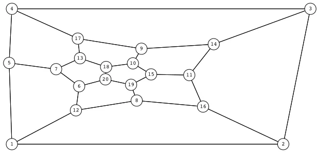
We show as example how to realize a dodecahedron using Algorithm 1. The graphGof the dodecahedron is particularly suitable for a good example, because every face of G is a pentagon. Thus we have to apply the more complicated part of the algorithm. Due to the symmetry ofGit does not matter which face we select as the boundary face. We follow our convention and name the vertices such thatv1, . . . , v5 belong tofb in cyclic order.
We start with a plane drawing (the pre-embedding) ofGwith strictly convex faces and no vertical edges. Figure 1 shows our choice. The pre-embedding induces an order of the vertices which we use to define thex-coordinates, namely
1 2
Figure 1: The pre-embedding of the dodecahedron.
The boundary x-coordinates are selected according to the algorithm. Next we construct the stress ω. We select some x-monotone paths and compute the induced costs for the interior edges. The stressω induces the matrix ˜L, which encodes the substitution stress by its off-diagonal entries (multiplied with -1). In our example we obtain
0.234791 −0.0769685 −0.0815444 −0.0354125 −0.0408658 −0.0769685 0.410969 −0.264196 −0.0401058 −0.02969
−0.0815444 −0.264196 0.506504 −0.108953 −0.05181
−0.0354125 −0.0401058 −0.108953 0.215884 −0.031412 −0.0408658 −0.02969 −0.05181 −0.031412 0.153786
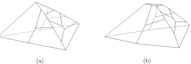
It can be observed that the entries ˜l35 and ˜l25 are not the dominating entries. But for the correctness of the algorithm this is required. Indeed, for our current “choice” of the substitution stress, we would obtain the embedding shown in Figure 2(a). The figure illustrates that the too small substitution stress entries ˜
ω25 and ˜ω35 cause a non-convex boundary facefb. Fortunately, we can fix the
problem by picking twox-monotone paths P25 and P35 and incrementing the costs on its edges byK (step 2 of the algorithm). We chooseK according to Lemma 5. Since in our casen= 20, ∆x= 36,α= 3, andk= 5, it suffices to setK= 260 400. The modified stressω gives now
˜
0.319465 −0.151322 −0.0666023 −0.00126453 −0.100277 −0.151322 7.1641 −2.97443 −0.0515457 −3.9868
−0.066602 −2.97443 7.22698 −0.144387 −4.04156
−0.001264 −0.0515457 −0.144387 0.275482 −0.0782853 −0.100277 −3.9868 −4.04156 −0.0782853 8.20693 fore, we can continue with the algorithm and choose yB as described in
(a) (b)
Figure 2: Embedding without (a) and with (b) making ˜ω25and ˜ω35dominant.
corresponding lifting is depicted in Figure 3(a). We did not execute the final scaling to obtain a more illustrative picture. Every face in the picture is drawn as strictly convex polygon. However, since we chose such a high value forK some edges become almost collinear. A more “spherical” embedding can be obtained by lowering the value forKand check whether this leavesy3−y2>1. Such a drawing (forK= 10) is shown in Figure 3(b).
(a) (b)
Figure 3: The final embedding (a) and the induced embedding forK= 10 (b).
Acknowledgments
References
[1] K. Buchin and A. Schulz. On the number of spanning trees a planar graph can have. In M. de Berg and U. Meyer, editors,ESA (1), volume 6346 of
Lecture Notes in Computer Science, pages 110–121. Springer, 2010. [2] M. Chrobak, M. T. Goodrich, and R. Tamassia. Convex drawings of graphs
in two and three dimensions (preliminary version). In12th Symposium on Computational Geometry, pages 319–328, 1996.
[3] D. Coppersmith and S. Winograd. Matrix multiplication via arithmetic progressions. J. Symb. Comput., 9(3):251–280, 1990.
[4] H. Crapo and W. Whiteley. Plane self stresses and projected polyhedra I: The basic pattern. Structural Topology, 20:55–78, 1993.
[5] G. Das and M. T. Goodrich. On the complexity of optimization problems for 3-dimensional convex polyhedra and decision trees. Comput. Geom. Theory Appl., 8(3):123–137, 1997.
[6] H. de Fraysseix, J. Pach, and R. Pollack. How to draw a planar graph on a grid. Combinatorica, 10(1):41–51, 1990.
[7] P. Eades and P. Garvan. Drawing stressed planar graphs in three dimen-sions. In F.-J. Brandenburg, editor,Graph Drawing, volume 1027 ofLecture Notes in Computer Science, pages 212–223. Springer, 1995.
[8] S. J. Gortler, C. Gotsman, and D. Thurston. Discrete one-forms on meshes and applications to 3d mesh parameterization. Computer Aided Geometric Design, 23(2):83–112, 2006.
[9] J. E. Hopcroft and P. J. Kahn. A paradigm for robust geometric algorithms.
Algorithmica, 7(4):339–380, 1992.
[10] R. J. Lipton, D. Rose, and R. Tarjan. Generalized nested dissection.SIAM J. Numer. Anal., 16(2):346–358, 1979.
[11] R. J. Lipton and R. E. Tarjan. Applications of a planar separator theorem.
SIAM J. Comput., 9(3):615–627, 1980.
[12] J. C. Maxwell. On reciprocal figures and diagrams of forces. Phil. Mag. Ser., 27:250–261, 1864.
[13] A. Rib´o Mor, G. Rote, and A. Schulz. Embedding 3-polytopes on a small grid. InSCG’07: Proc. 23rd Annual Symposium on Computational Geom-etry, pages 112–118, New York, NY, USA, 2007. ACM.
[14] A. Rib´o Mor, G. Rote, and A. Schulz. Small grid embeddings of 3-polytopes.
[15] J. Richter-Gebert. Realization Spaces of Polytopes, volume 1643 ofLecture Notes in Mathematics. Springer, 1996.
[16] W. Schnyder. Embedding planar graphs on the grid. InProc. 1st ACM-SIAM Sympos. Discrete Algorithms, pages 138–148, 1990.
[17] O. Schramm. Existence and uniqueness of packings with specified combi-natorics. Israel J. Math., 73:321–341, 1991.
[18] P. R. Scott and P. W. Awyong. Inequalities for convex sets. J. Ineq. Pure and Appl. Math., 1(1), 2000.
[19] E. Steinitz. Encyclop¨adie der mathematischen Wissenschaften. InPolyeder und Raumteilungen, pages 1–139. 1922.
[20] W. T. Tutte. Convex representations of graphs.Proceedings London Math-ematical Society, 10(38):304–320, 1960.
[21] W. T. Tutte. How to draw a graph. Proceedings London Mathematical Society, 13(52):743–768, 1963.
[22] W. Whiteley. Motion and stresses of projected polyhedra.Structural Topol-ogy, 7:13–38, 1982.
[23] H. Whitney. A set of topological invariants for graphs. Amer. J. Math., 55:235–321, 1933.