Directory UMM :wiley:Public:college:hill:

(1)

Copyright 1996 Lawrence C. Marsh

1.0

PowerPoint Slides for

Undergraduate Econometrics

by

Lawrence C. Marsh

To accompany: Undergraduate Econometrics

by Carter Hill, William Griffiths and George Judge

(2)

1

Copyright 1996 Lawrence C. Marsh

The Role of

Econometrics

in Economic Analysis

Chapter 1

Copyright © 1997 John Wiley & Sons, Inc. All rights reserved. Reproduction or translation of this work beyond that permitted in Section 117 of the 1976 United States Copyright Act without the express written permission of the copyright owner is unlawful. Request for further information should be addressed to the Permissions Department, John Wiley & Sons, Inc. The purchaser may make back-up copies for his/her own use only and not for distribution or resale. The Publisher assumes no responsibility for errors, omissions, or damages, caused by the use of these programs or from the use of the information contained herein.

Using Information:

1. Information from

economic theory.

2. Information from

economic data.

The Role of Econometrics

1.2

Copyright 1996 Lawrence C. Marsh

Understanding Economic Relationships:

federal budget

Dow-Jones Stock Index

trade

deficit _{Federal Reserve}

Discount Rate

capital gains tax

rent control laws short term treasury bills

power of labor unions

crime rate inflation

unemployment

money supply

economic theory

economic data

}

economic decisions

To use information effectively:

*Econometrics* helps us combine economic theory and economic data .

Economic Decisions

1.4

Copyright 1996 Lawrence C. Marsh

Consumption, c, is some function of income, i :

c = f(i)

For applied econometric analysis this consumption function must be specified more precisely.

The Consumption Function

1.5

Copyright 1996 Lawrence C. Marsh

demand, qd_{, for an individual commodity:}

qd_{= f( p, p}c_{, p}s_{, i )}

supply, qs_{, of an individual commodity:}

qs_{= f( p, p}c_{, p}f₎

p = own price; pc_{= price of complements;}

ps_{= price of substitutes; i = income}

p = own price; pc_{= price of competitive products;}

ps_{= price of substitutes; p}f_{= price of factor inputs}

demand

(3)

2

Copyright 1996 Lawrence C. Marsh

Listing the variables in an economic relationship is not enough.

For effective policy we must know the amount of change

needed for a policy instrument to bring about the desired effect:

How much ?

• By how much should the Federal Reserve raise interest rates to prevent inflation?

• By how much can the price of football tickets be increased and still fill the stadium?

Answering the How Much? question

Need to estimate parameters that are both:

1. unknown and

2. unobservable

1.8

Copyright 1996 Lawrence C. Marsh

Average or systematic behavior over many individuals or many firms.

Not a single individual or single firm. Economists are concerned with the unemployment rate and not whether a particular individual gets a job.

The Statistical Model

Actual vs. Predicted Consumption:

Actual = systematic part + random error

Systematic part provides prediction, f(i), but actual will miss by random error, e. Consumption, c, is function, f, of income, i, with error, e:

c = f(i) + e

1.10

Copyright 1996 Lawrence C. Marsh

c = f(i) + e

Need to define f(i) in some way.

To make consumption, c, a linear function of income, i :

f(i) = β1 + β2 i

The statistical model then becomes: c = β₁ + β₂ i + e

The Consumption Function

• Dependent variable , y, is focus of study

(predict or explain changes in dependent variable).

• Explanatory variables, X2 and X3, help us explain observed changes in the dependent variable.

y = β1 + β2 X2 + β3 X3 + e

The Econometric Model

(4)

3

Copyright 1996 Lawrence C. Marsh Statistical Models

Controlled (experimental) vs.

Uncontrolled (observational)

Uncontrolled experiment (econometrics) explaining consump-tion, y : price, X2, and income, X3, vary at the same time. Controlled experiment (“pure” science) explaining mass, y : pressure, X2, held constant when varying temperature, X3, and vice versa.

Econometric

model

• economic model

economic variables and parameters.

• statistical model

sampling process with its parameters.

• data

observed values of the variables.

1.14

Copyright 1996 Lawrence C. Marsh

• Uncertainty regarding an outcome.

• Relationships suggested by economic theory. • Assumptions and hypotheses to be specified. • Sampling process including functional form. • Obtaining data for the analysis.

• Estimation rule with good statistical properties. • Fit and test model using software package. • Analyze and evaluate implications of the results. • Problems suggest approaches for further research.

The Practice of Econometrics

Note: the textbook uses the following symbol to mark sections with advanced material

:

“Skippy”

1.16

Copyright 1996 Lawrence C. Marsh

Some Basic

Probability

Concepts

Chapter 2

random variable:

A variable whose value is unknown until it is observed. The value of a random variable results from an experiment.

The term random variable implies the existence of some known or unknown probability distribution defined over the set of all possible values of that variable.

In contrast, an arbitrary variable does not have a probability distribution associated with its values.

(5)

4

Copyright 1996 Lawrence C. Marsh

Controlled experiment values of explanatory variables are chosen with great care in accordance with an appropriate experimental design.

Uncontrolled experiment values of explanatory variables consist of nonexperimental observations over which the analyst has no control.

discrete random variable:

A discrete random variable can take only a finite number of values, that can be counted by using the positive integers.

Example: Prize money from the following lottery is a discrete random variable:

first prize: $1,000 second prize: $50 third prize: $5.75

since it has only four (a finite number) (count: 1,2,3,4) of possible outcomes:

$0.00; $5.75; $50.00; $1,000.00

Discrete Random Variable

2.4

Copyright 1996 Lawrence C. Marsh

continuous random variable: A continuous random variable can take any real value (not just whole numbers) in at least one interval on the real line.

Examples:

Gross national product (GNP) money supply

interest rates price of eggs household income expenditure on clothing

Continuous Random Variable

2.5

Copyright 1996 Lawrence C. Marsh

A discrete random variable that is restricted to two possible values (usually 0 and 1) is called a dummy variable (also, binary or indicator variable).

Dummy variables account for qualitative differences: gender (0=male, 1=female),

race (0=white, 1=nonwhite), citizenship (0=U.S., 1=not U.S.), income class (0=poor, 1=rich).

Dummy Variable

2.6

Copyright 1996 Lawrence C. Marsh

A list of all of the possible values taken by a discrete random variable along with their chances of occurring is called a probability function or probability density function (pdf).

die x f(x)

one dot 1 1/6 two dots 2 1/6 three dots 3 1/6 four dots 4 1/6 five dots 5 1/6 six dots 6 1/6

A discrete random variable X has pdf, f(x), which is the probability

that X takes on the value x.

f(x) = P(X=x)

0 < f(x) < 1

If X takes on the n values: x1, x2, . . . , xn,

then f(x1) + f(x2)+. . .+f(xn) = 1.

Therefore,

(6)

5

0 1 2 3 X

number, X, on Dean’s List of three roommates f(x)

0.2 0.4

0.1 0.3

A continuous random variable uses

area under a curve rather than the height, f(x), to represent probability:

f(x)

X $34,000. $55,000. per capita income, X, in the United States

0.1324 0.8676

red area

green area

2.10

Copyright 1996 Lawrence C. Marsh

Since a continuous random variable has an

uncountably infinite number of values, the probability of one occurring is zero.

P [ X = a ] = P [ a < X < a ] = 0

Probability is represented by area. Height alone has no area. An interval for X is needed to get

an area under the curve.

P [ a < X < b ] =

∫

f(x) dx

b

a

The area under a curve is the integral of the equation that generates the curve:

For continuous random variables it is the integral of f(x), and not f(x) itself, which defines the area and, therefore, the probability.

2.12

Copyright 1996 Lawrence C. Marsh

n

Rule 2: Σ axi = a Σxi i = 1 i = 1

n

Rule 1: Σxi = x1 + x2 + . . . + xn i = 1

n

Rule 3: _Σ (x_i +y_i) = _Σx_i + _Σy_i

i = 1 i = 1 i = 1

n n n

Note that summation is a linear operator which means it operates term by term.

Rules of Summation

2.13

Copyright 1996 Lawrence C. Marsh

Rule 4: _Σ (ax_i +by_i) = a _Σx_i + b _Σy_i

i = 1 i = 1 i = 1

n n n

Rules of Summation (continued)

Rule 5: x = Σxi = i = 1

n n

1 x1 + x2 + . . . + xn

n

The definition of x as given in Rule 5 implies the following important fact:

Σ (xi− x) = 0 i = 1

n

(7)

6

Copyright 1996 Lawrence C. Marsh

Rule 6: _Σf(x_i) = f(x₁) + f(x₂) + . . . + f(x_n)

i = 1

n

Notation: Σf(xi) = Σf(xi) = Σf(xi)

n x i i = 1

n

Rule 7: Σ Σ f(xi,yj) = Σ [ f(xi,y1) + f(xi,y2)+. . .+ f(xi,ym)] i = 1 i = 1

n m

j = 1

The order of summation does not matter :

Σ Σ f(xi,yj) = Σ Σ f(xi,yj) i = 1

n m

j = 1 j = 1

m n

i = 1

Rules of Summation (continued)

The

mean

or arithmetic average of a

random variable is its mathematical

expectation or expected value, EX.

The Mean of a Random Variable

2.16

Copyright 1996 Lawrence C. Marsh

Expected Value

There are two entirely different, but mathematically equivalent, ways of determining the expected value:

1. Empirically:

The expected value of a random variable, X, is the average value of the random variable in an infinite number of repetitions of the experiment.

In other words, draw an infinite number of samples, and average the values of X that you get.

Expected Value

2. Analytically:

The expected value of a discrete random variable, X, is determined by weighting all the possible values of X by the corresponding probability density function values, f(x), and summing them up.

E[X] = x₁f(x₁) + x₂f(x₂) + . . . + x_nf(x_n)

In other words:

2.18

Copyright 1996 Lawrence C. Marsh

In the empirical case when the

sample goes to infinity the values

of X occur with a frequency

equal to the corresponding f(x)

in the analytical expression.

As sample size goes to infinity, the

empirical and analytical methods

will produce the same value.

Empirical vs. Analytical

x =

Σ

xi

n i = 1

where n is the number of sample observations.

Empirical (sample) mean:

E[X] =

Σ

xif(xi)

i = 1 n

where n is the number of possible values of xi.

Analytical mean:

Notice how the meaning of n changes.

(8)

7

E X =

Σ

xi f(xi)

i=1

n

The expected value of X-squared:

E X =

Σ

xi f(xi)

i=1

n

2 ₂

It is important to notice thatf(xi) does not change!

The expected value of X-cubed:

E X =

Σ

xi f(xi)

i=1

n

3 ₃

The expected value of X:

EX = 0 (.1) + 1 (.3) + 2 (.3) + 3 (.2) + 4 (.1)

2

EX = 0 (.1) + 1 (.3) + 2 (.3) + 3 (.2) + 4 (.1) 2 2 2 2 2

= 1.9

= 0 + .3 + 1.2 + 1.8 + 1.6

= 4.9

3

EX = 0 (.1) + 1 (.3) + 2 (.3) + 3 (.2) +4 (.1)3 3 3 3 3 = 0 + .3 + 2.4 + 5.4 + 6.4

= 14.5

2.22

E[g(X)]

=

Σ

g

(

xi

)

f(xi)

n i = 1

g(X) = g1(X) + g2(X)

E[g(X)]

=

Σ [

g1(xi) + g2(xi)]f(xi)

n i = 1

E[g(X)]

=

Σ

g1(xi)f(xi) +

Σ

g2(xi)f(xi)

n i = 1

E[g(X)]

=

E[g1(X)] + E[g2(X)]

Adding

and

Subtracting

Random Variables

E(X-Y) = E(X) - E(Y)

E(X+Y) = E(X) + E(Y)

2.24

Copyright 1996 Lawrence C. Marsh

E(X+a) = E(X) + a

Adding

a

constant

to a variable will

add a constant to its expected value:

Multiplying by

constant

will multiply

its expected value by that constant:

E(bX) = b E(X)

var(X) = average squared deviations around the mean of X.

var(X) = expected value of the squared deviations around the expected value of X.

var(X) =E [(X - EX) ] 2

(9)

8

Copyright 1996 Lawrence C. Marsh

var(X) =E [(X - EX) ]

=E [X - 2XEX + (EX) ]

2 2

2

=E(X ) - 2 EX EX + E (EX)

2 2

=E(X ) - 2 (EX) + (EX) 2 2 2 =E(X ) - (EX) 2 2

var(X) =E [(X - EX) ] 2

var(X) = E(X ) - (EX) 2 2

variance

of a discrete

random variable, X:

standard deviation is square root of variance

var ( X ) =

(x

_i

- EX )

2

f(x

_i

)

i = 1 n

∑

2.28

Copyright 1996 Lawrence C. Marsh

x_i f(x_i) (x_i - EX) (x_i - EX) f(x_i)

2 .1 2 - 4.3 = -2.3 5.29 (.1) = .529

3 .3 3 - 4.3 = -1.3 1.69 (.3) = .507

4 .1 4 - 4.3 = - .3 .09 (.1) = .009

5 .2 5 - 4.3 = .7 .49 (.2) = .098

6 .3 6 - 4.3 = 1.7 2.89 (.3) = .867

Σ x_i f(x_i) = .2 + .9 + .4 + 1.0 + 1.8 = 4.3

Σ (x_i - EX) f(x_i) = .529 + .507 + .009 + .098 + .867 = 2.01

2

calculate the variance for a

discrete random variable, X:

i = 1 n

n i = 1

Z = a + cX

var(Z) = var(a + cX)

= E [(a+cX) - E(a+cX)]

= c var(X)

2

var(a + cX) = c var(X)

2

2.30

Copyright 1996 Lawrence C. Marsh

A

joint

probability density function,

f(x,y), provides the probabilities

associated with the joint occurrence

of all of the possible pairs of X and Y.

Joint pdf

2.31

Copyright 1996 Lawrence C. Marsh

college grads in household

.15

.05

.45

.35

joint pdf

f(x,y)

Y = 1 Y = 2

vacation homes owned

X = 0

X = 1

Survey of College City, NY

f

(0,1)

f

(0,2)

f

(1,1)

f

(1,2)

(10)

9

Copyright 1996 Lawrence C. Marsh

E[g(X,Y)] =

Σ

g(x

_i

,y

_j

) f(x

_i

,y

_j

)

i j

E(XY) = (0)(1)(.45)+(0)(2)(.15)+(1)(1)(.05)+(1)(2)(.35)=.75

E(XY) =

Σ

_i

Σ

x

i

y

j

f(x

i

,y

j

)

j

Calculating the expected value of

functions of two random variables.

The

marginal

probability density functions,

f(x) and f(y), for discrete random variables,

can be obtained by summing over the f(x,y)

with respect to the values of Y to obtain f(x)

with respect to the values of X to obtain f(y).

f(x

i

) =

Σ

f(x

i

,y

j

)

f(y

j

) =

Σ

f(x

i

,y

j

)

i j

Marginal pdf

2.34

Copyright 1996 Lawrence C. Marsh

.15

.05

.45

.35

marginal

Y = 1 Y = 2

X = 0

X = 1

.60

.40

.50

f

(X = 1)

f

(X = 0)

f

(Y = 1)

f

(Y = 2)

marginal pdf for Y:

marginal pdf for X:

The

conditional

probability density

functions of X given Y=y , f(x

|

y),

and of Y given X=x , f(y

|

x),

are obtained by dividing f(x,y) by f(y)

to get f(x

|

y) and by f(x) to get f(y

|

x).

f(x

|

y) =

f(x,y)

f(y

|

x) =

f(x,y)

f(y)

f(x)

Conditional pdf

2.36

Copyright 1996 Lawrence C. Marsh

.15

.05

.45

.35

conditonal

Y = 1 Y = 2

X = 0

X = 1

.60

.40

.50

.25 .75

.875 .125 .90

.10 .70

.30

f(Y=2_|X= 0)=.25

f(Y=1|X = 0)=.75

f(Y=2|X = 1)=.875

f(X=0|Y=2)=.30

f(X=1_|Y=2)=.70

f(X=0|Y=1)=.90

f(X=1_|Y=1)=.10

f(Y=1|X = 1)=.125

X and Y are

independent

random

variables if their joint pdf, f(x,y),

is the product of their respective

marginal pdfs, f(x) and f(y) .

f(x

i

,y

j

) = f(x

i

) f(y

j

)

for independence this must hold for all pairs of i and j

(11)

10

Copyright 1996 Lawrence C. Marsh

.15

.05

.45

.35

not independent

Y = 1 Y = 2

X = 0

X = 1

.60

.40

.50

f

(X = 1)

f

(X = 0)

f

(Y = 1)

f

(Y = 2)

marginal pdf for Y:

marginal pdf for X: .50x.60=.30 .50x.60=.30

.50x.40=.20 .50x.40=.20

The calculations in the boxes show the numbers required to have

independence.

The

covariance

between two random

variables, X and Y, measures the

linear association between them.

cov(X,Y) = E[(X - EX)(Y-EY)]

Note that variance is a special case of covariance.

cov(X,X) = var(X) = E[(X - EX) ]

2

Covariance

2.40

Copyright 1996 Lawrence C. Marsh

cov(X,Y) =E [(X - EX)(Y-EY)]

=E [XY - X EY - Y EX + EX EY]

=E(XY) - 2 EX EY + EX EY

=E(XY) - EX EY

cov(X,Y) =E [(X - EX)(Y-EY)]

cov(X,Y) = E(XY) - EX EY

=E(XY) - EX EY - EY EX + EX EY

.15

.05

.45

.35

Y = 1 Y = 2

X = 0

X = 1

.60

.40

.50

EX=0(.60)+1(.40)=.40 EY=1(.50)+2(.50)=1.50

E(XY) = (0)(1)(.45)+(0)(2)(.15)+(1)(1)(.05)+(1)(2)(.35)=.75

EX EY = (.40)(1.50) = .60

cov(X,Y) = E(XY) - EX EY = .75 - (.40)(1.50) = .75 - .60 = .15

covariance

2.42

Copyright 1996 Lawrence C. Marsh

The

correlation

between two random

variables X and Y is their covariance

divided by the square roots of their

respective variances.

Correlation is a pure number falling between -1 and 1.

cov(X,Y)

ρ

(X,Y) =

var(X) var(Y)

Correlation

2.43

Copyright 1996 Lawrence C. Marsh

.15

.05

.45

.35

Y = 1 Y = 2

X = 0

X = 1

.60

.40

.50

EX=.40 EY=1.50

cov(X,Y) = .15

correlation

EX=0(.60)+1(.40)=2 2 2 .40

var(X) = E(X ) - (EX) = .40 - (.40) = .24

2 2 2

EY=1(.50)+2(.50) = .50 + 2.0 = 2.50

2 2 2

var(Y) = E(Y ) - (EY) = 2.50 - (1.50) = .25

2 2 2

ρ(X,Y) = cov(X,Y)

var(X) var(Y)

(12)

11

Copyright 1996 Lawrence C. Marsh

Independent random variables

have zero covariance and,

therefore, zero correlation.

The converse is not true.

Zero Covariance & Correlation

The expected value of the weighted sum

of random variables is the sum of the

expectations of the individual terms.

Since expectation is a linear operator, it can be applied term by term.

E[c

1

X + c

2

Y] = c

1

EX + c

2

EY

E[c

1

X

1

+...+ c

n

X

n

] = c

1

EX

1

+...+ c

n

EX

n In general, for random variables X1, . . . , Xn :

2.46

variables is the sum of the variances, each times the square of the weight, plus twice the covariances of all the random variables times the products of their weights.

var(c1X + c2Y)=c1 var(X)+c2 var(Y) + 2c1c2cov(X,Y)

2 2

var(c₁X − c2Y) = c21 var(X)+c2 2var(Y) − 2c1c2cov(X,Y) Weighted sum of random variables:

Weighted difference of random variables:

The Normal Distribution

Y ~ N(

β

,

σ

2

)

f(y) =

2

π

σ

2

1

exp

β

y

f(y)

2

σ

2

(y -

β

)

2

-2.48

Copyright 1996 Lawrence C. Marsh

The Standardized Normal

Z ~ N(

0

,

1

)

f(z) =

2

π

1

exp

-

2

z

2

Z = (y -

β

)/

σ

P [ Y > a ] = P > = P Z > Y - _σβ a - _σβ a - _σβ

β

y

f(y)

a

(13)

12

Copyright 1996 Lawrence C. Marsh

P [ a < Y < b ] = P < <

= P < Z < a - β Y - β

σ

σ b - σβ

a - β

σ

b - β

σ

β

y

f(y)

a

Y ~ N(

β

,

σ

2

)

b

Y1 ~ N(β1,σ12), Y2 ~ N(β2,σ22), . . . , Yn ~ N(βn,σn2)

W = c

1

Y

1

+ c

2

Y

2

+ . . . + c

n

Y

n

Linear combinations of jointly

normally distributed random variables

are themselves normally distributed.

W ~ N

[

E(W), var(W)

]

2.52

Copyright 1996 Lawrence C. Marsh

mean: E[V] = E[

χ

(m) ] = m

If Z1, Z2, . . . , Zm denote m independent

N(0,1) random variables, and

V = Z2₁+ Z2₂ + . . . + Z2_m, then V ~

χ

_(m)2 V is chi-square with m degrees of freedom.

Chi-Square

variance: var[V] = var[

χ

(m) ] = 2m

If Z1, Z2, . . . , Zm denote m independent

N(0,1) random variables, and

V = Z2₁+ Z2₂ + . . . + Z2_m, then V ~

χ

_(m)2 V is chi-square with m degrees of freedom.

2

mean: E[

t

] = E[

t

(m) ] = 0 symmetric about zero

variance: var[

t

] = var[

t

(m) ] = m / (m

−

2)

If Z ~ N(0,1) and V ~

χ

(m) and if Z and V

are independent then,

~

t

(m)

t

is student-t with m degrees of freedom. 2

t =

Z

V _m

Student - t

2.54

Copyright 1996 Lawrence C. Marsh

If V1 ~

χ

(m

1) and V2 ~

χ

(m2) and if V1 and V2 are independent, then

~ F

(m 1,m2)

F

is an F statistic with m1 numerator

degrees of freedom and m2 denominator

degrees of freedom. 2

F =

V_{1 m}

1 V2

m 2

2

F Statistic

2.55

Copyright 1996 Lawrence C. Marsh

The Simple Linear

Regression

Model

Chapter 3

(14)

13

Copyright 1996 Lawrence C. Marsh

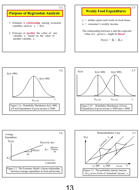
1. Estimate a relationship among economic variables, such as y = f(x).

2. Forecast or predict the value of one variable, y, based on the value of another variable, x.

Purpose of Regression Analysis

Weekly Food Expenditures

y = dollars spent each week on food items. x = consumer’s weekly income.

The relationship between x and the expected value of y , given x, might be linear:

E(y|x) = β1 + β2 x

3.3

f(y|x=480)

y µy|x=480

Figure 3.1a Probability Distribution f(y|x=480) of Food Expenditures if given income x=$480.

f(y|x=480) f(y|x=800)

[image:14.612.72.537.92.726.2]

y µy|x=480 µy|x=800

Figure 3.1b Probability Distribution of Food Expenditures if given income x=$480 and x=$800.

3.5

Copyright 1996 Lawrence C. Marsh

{

β1

∆x

∆E(y|x) E(y|x)

Average Expenditure

x (income) E(y|x)=β1+β2x

β2=

∆E(y|x) ∆x

Figure 3.2 The Economic Model: a linear relationship between avearage expenditure on food and income.

.

xt

x1=480 x2=800

yt

f(yt)

Figure 3.3. The probability density function for yt at two levels of household income, xt

expenditure

Homoskedastic Case

income

(15)

14

Copyright 1996 Lawrence C. Marsh

.

xt

x1 x2

[image:15.612.75.540.94.724.2]

yt f(yt)

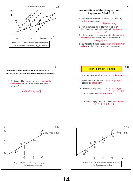
Figure 3.3+. The variance of yt increases

as household income, xt , increases. expenditure

Heteroskedastic Case

x3

.

income

Assumptions of the Simple Linear

Regression Model - I

1. The average value of y, given x, is given by the linear regression:

E(y) = β1 + β2x

2. For each value of x, the values of y are distributed around their mean with variance:

var(y) = σ2

3. The values of y are uncorrelated, having zero covariance and thus no linear relationship:

cov(yi ,yj) = 0

4. The variable x must take at least two different values, so that x ≠ c, where c is a constant.

3.9

5. (optional) The values of y are normally distributed about their mean for each value of x:

y ~ N [(β1+β2x), σ2 ]

One more assumption that is often used in practice but is not required for least squares:

The Error Term

y is a random variable composed of two parts:

I. Systematic component: E(y) = β1 + β2x

This is the mean of y.

II. Random component: e = y - E(y) = y - β1 - β2x

This is called the random error.

Together E(y) and e form the model:

y = β1 + β2x + e

3.11

Figure 3.5 The relationship among y, e and the true regression line.

.

y4 y1 y2 y3

x1 x2 x3 x4

}

{

e1 e2 e3

e4 E(y) = β₁+ β₂x

x

}

.

}

.

y4 y1

y2 _y

3

x1 x2 x3 x4

[image:15.612.77.291.108.262.2]

{

e1 e2 e3 e4 x y

Figure 3.7a The relationship among y, e and the fitted regression line.

^

y = b1 + b2x

(16)

15

Copyright 1996 Lawrence C. Marsh

{

.

y4

y1

y2 y₃

x1 x2 x3 x4 _x

[image:16.612.77.535.95.704.2]

y

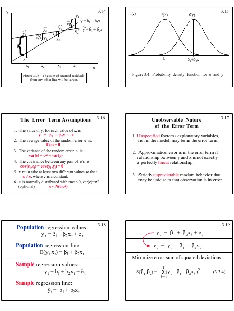
Figure 3.7b The sum of squared residuals from any other line will be larger.

y = b1 + b2x

^

.

y1

^

y3

^

y4

^ y = b^* *1 + b*2x *

e1

^*

e2

^*

y2

^*

e3

^* * e^*4

*

{

3.14 _f(

.

f(e) f(y)

Figure 3.4 Probability density function for e and y

0 _β₁₊_β₂_x

3.15

The Error Term Assumptions

1. The value of y, for each value of x, is y = β1 + β2x + e

2. The average value of the random error e is:

E(e) = 0

3. The variance of the random error e is:

var(e) = σ2 = var(y)

4. The covariance between any pair of e’s is:

cov(ei ,ej) = cov(yi ,yj) = 0

5. x must take at least two different values so that

x ≠ c, where c is a constant.

6. e is normally distributed with mean 0, var(e)=σ2

(optional) e ~ N(0,σ2₎

3.16

Unobservable Nature

of the Error Term

1. Unspecified factors / explanatory variables, not in the model, may be in the error term.

2. Approximation error is in the error term if relationship between y and x is not exactly a perfectly linear relationship.

3. Strictly unpredictable random behavior that may be unique to that observation is in error.

3.17

Copyright 1996 Lawrence C. Marsh

Population

regression values:

y

_t

=

β

₁

+

β

₂

x

_t

+ e

_t

Population

regression line:

E(y

t

|x

t

) =

β

1

+

β

2

x

t

Sample

regression values:

y

t

= b

1

+ b

2

x

t

+ e

t

Sample

regression line:

y

t

= b

1

+ b

2

x

t

^

y

t

=

β

1

+

β

2

x

t

+ e

t

Minimize error sum of squared deviations:

S(

β

₁

,

β

₂) =

Σ

(

y

_t

-

β

₁

-

β

₂

x

_t)2 (3.3.4)

t=1 T

e

t

= y

t

-

β

1

-

β

2

x

t [image:16.612.320.533.108.224.2]

(17)

16

Copyright 1996 Lawrence C. Marsh

Minimize w.

r.

t.

β

₁

and

β

₂

:

S(

β

₁

,

β

₂) =

Σ

(

y

t

-

β

1

-

β

2

x

t)2 (3.3.4)

t =1 T

= - 2

Σ

(

y

_t

-

β

₁

-

β

₂

x

_t)

= - 2

Σ

x

t (

y

t

-

β

1

-

β

2

x

t)

∂S(

.

)

∂β

1 ∂S(

.

)

∂β

2

Set each of these two derivatives equal to zero and solve these two equations for the two unknowns:

β

₁

β

₂

S(.)

βi bi

.

Minimize w.

r.

t.

β

₁

and

β

₂

:

S(

.

) =

Σ

(

y

t

-

β

1

-

β

2

x

t)2

t =1 T

∂S(.) ∂βi

< 0

∂S(.) ∂βi

>0 ∂S(.)

∂βi

=0

3.21

Copyright 1996 Lawrence C. Marsh

To minimize S(.), you set the two derivatives equal to zero to get:

= - 2

Σ

(

y

t

-

b

1

-

b

2

x

t) = 0

= - 2

Σ

x

t (

y

t

-

b

1

-

b

2

x

t) = 0

∂S(

.

)

∂β

1 ∂S(

.

)

∂β

2

When these two terms are set to zero,

β

1 and

β

2 become

b

1 and

b

2 because they no longer represent just any value of

β

₁ and

β

₂ but the special

values that correspond to the minimum of S(

.

) .

- 2

Σ

(

y

t

-

b

1

-

b

2

x

t) = 0

- 2

Σ

x

t (

y

t

-

b

1

-

b

2

x

t) = 0

Σ

y

t-

T

b

1-

b

2

Σ

x

t = 0

Σ

x

_t

y

_t-

b

₁

Σ

x

_t-

b

₂

Σ

x

_t2 = 0

T

b

₁+

b

₂

Σ

x

t =

Σ

y

t

b

1

Σ

x

t +

b

2

Σ

x

t =

Σ

x

t

y

t

2

3.23

Solve for

b

₁ and

b

₂ using definitions of

x

and

y

T

b

₁+

b

₂

Σ

x

t =

Σ

y

t

b

₁

Σ

x

t +

b

2

Σ

x

t =

Σ

x

t

y

t

2

T

Σ

x

t

y

t -

Σ

x

t

Σ

y

t

T

Σ

x

t2

- (

Σ

x

t)2

b

₂=

b

₁= y -

b

₂

x

elasticities

percentage change in y percentage change in x

η = =

∆x/x ∆y/y

= _∆∆y x

x y

Using calculus, we can get the elasticity at a point:

η = lim ∆_∆y x =

x y

∂y x ∂x y

∆x→0

(18)

17

Copyright 1996 Lawrence C. Marsh

E(y) =

β

1

+

β

2

x

∂

E(y)

∂

x

=

β

2

applying elasticities

∂

E(y)

∂

x

=

β

2

η

=

E(y)

x

E(y)

x

estimating elasticities

∂

y

∂

x

=

b

2

η

=

y

x

y

x

^

y

t

=

b

1

+ b

2

x

t

= 4 + 1.5 x

t

^

x

= 8 = average number of years of experience

y

= $10 = average wage rate

= 1.5 = 1.2

8

10

=

b

₂

η

y

x

^

3.27

Copyright 1996 Lawrence C. Marsh

Prediction

y

^_t

= 4 + 1.5 x

_t

Estimated regression equation:

x

_t= years of experience

y

^t = predicted wage rate

If

x

t = 2 years, then

y

t =

$7.00

per hour

.

^

If

x

_t= 3 years, then y^_t

=

$8.50

per hour

.

log-log models

ln(y) =

β

₁

+

β

₂

ln(x)

∂

ln(y)

∂

x

∂

ln(x)

∂

x

=

β

₂

∂

y

∂

x

=

β

2

1

y

∂

x

∂

x

1

x

3.29

Copyright 1996 Lawrence C. Marsh

∂

y

∂

x

=

β

2

1

y

∂

x

∂

x

1

x

=

β

2

∂

y

∂

x

y

elasticity of y with respect to x:

=

β

₂

∂

y

∂

x

y

η

=

Properties of

Least

Squares

Estimators

Chapter 4

(19)

18

Copyright 1996 Lawrence C. Marsh

y

_t

=

household weekly food expenditures

Simple Linear Regression Model

y

_t

=

β

₁

+

β

₂

x

_t

+

ε

_t

x

_t

=

household weekly income

For a given level of

x

_t, the expected level of food expenditures will be:

E(

y

_t

|

x

_t)

=

β

₁

+

β

₂

x

_t

1.

y

_t

=

β

₁

+

β

₂

x

_t

+

ε

_t

2.

E(

ε

_t

)

=

0 <=> E(

y

_t

)

=

β

₁

+

β

₂

x

_t

3.

var(

ε

_t

)

=

σ

2

=

var(

y

t

)

4.

cov(

ε

_i

,

ε

_j

)

=

cov(

y

_i

,

y

_j

)

=

0

5.

x

_t

≠

c

for every observation

6.

ε

_t

~N(0,

σ

2

) <=>

y

t

~

N(

β

1

+

β

2

x

t

,

σ

2

)

Assumptions of the Simple

Linear Regression Model

4.3

Copyright 1996 Lawrence C. Marsh

The population parameters

β

₁and

β

₂ are unknown population constants

.

The formulas that produce the sample estimates b₁ and b₂ are called the estimators of

β

₁and

β

₂

.

When b₀ and b₁ are used to represent the formulas rather than specific values, they are called estimators of

β

₁and

β

₂ which are random variables because they are different from sample to sample.

• If the least squares estimators b0 and b1

are random variables, then what are their their means, variances, covariances and probability distributions?

• Compare the properties of alternative

estimators to the properties of the least squares estimators.

Estimators are Random Variables

( estimates are not )

4.5

Copyright 1996 Lawrence C. Marsh

The Expected Values of b1 and b2

The least squares formulas (estimators) in the simple regression case:

b

₂

=

T

Σ

x

t

y

t

-

Σ

x

t

Σ

y

t

T

Σ

x

_t2

-(

Σ

x

_t

)

2

b

₁

= y - b

₂

x

where

y =

Σ

y

_t

/ T

and

x =

Σ

x

_t

/ T

(3.3.8a)

(3.3.8b)

4.6 Substitute in

y

=

β

₁

+

β

₂

x

_t

+

ε

_t to get:

b

₂

=

β

₂

+

T

Σ

x

t

ε

t

-

Σ

x

t

Σε

t

T

Σ

x

_t2

-(

Σ

x

_t

)

2

The mean of

b

₂ is:

Eb

₂

=

β

₂

+

T

Σ

x

t

E

ε

t

-

Σ

x

t

Σ

E

ε

t

T

Σ

x

_t2

-(

Σ

x

_t

)

2

(20)

19

Copyright 1996 Lawrence C. Marsh

The result

Eb

₂

=

β

₂ means that the distribution of

b

₂ is centered at

β

₂.

Since the distribution of

b

₂ is centered at

β

₂ ,we say that

b

₂is an unbiased estimator of

β

₂.

An Unbiased Estimator

4.8

Copyright 1996 Lawrence C. Marsh

The unbiasedness result on the

previous slide assumes that we

are using the

correct model

.

If the model is of the wrong form

or is missing important variables,

then

E

ε

_t

≠

0

, then

Eb

₂

≠

β

₂

.

Wrong Model Specification

4.9

Copyright 1996 Lawrence C. Marsh

Unbiased Estimator of the Intercept

In a similar manner, the estimator b

₁

of the intercept or constant term can be

shown to be an

unbiased

estimator of

β

₁

when the model is correctly specified.

Eb

₁

=

β

₁

b

₂

=

T

Σ

x

t

y

t

−

Σ

x

t

Σ

y

t

T

Σ

x

_t2

−

(

Σ

x

_t

)

2 (3.3.8a)

(4.2.6)

Equivalent expressions for b

₂

:

Expand and multiply top and bottom by T:

b

₂

=

Σ

(x

t

−

x )

(

y

t

−

y )

Σ(

x

_t

−

x

)

2

4.11

Copyright 1996 Lawrence C. Marsh

Variance of b

₂

Given that both yt and

ε

t have variance

σ

2, the variance of the estimator b2 is:

b2 is a function of the yt values but var(b2) does not involve yt directly.

Σ(

x

_t

−

x

)

σ

2

var(b

₂

) =

Variance of b

₁

Τ Σ(

x

_t

−

x

)

2

var(b

₁

) =

σ

2

Σ

x

_t2 the variance of the estimator b1 is:

b

₁

= y

−

b

₂

x

Given

(21)

20

Copyright 1996 Lawrence C. Marsh

Covariance of b

₁

and b

₂

Σ(

x

_t

−

x

)

2

cov(b

₁

,b

₂

) =

σ

2

−

x

If x = 0, slope can change without affecting the variance.

4.14

What factors determine

variance and covariance ?

1. σ 2: uncertainty about y

t values uncertainty about b1, b2 and their relationship. 2. The more spread out the xt values are then the more

confidence we have in b1, b2, etc. 3. The larger the sample size, T, the smaller the

variances and covariances. 4. The variance b1 is large when the (squared) xt values

are far from zero (in either direction). 5. Changing the slope, b2, has no effect on the intercept,

b1, when the sample mean is zero. But if sample mean is positive, the covariance between b1 and b2 will be negative, and vice versa.

4.15

Gauss-Markov Theorm

Under the first five assumptions of the simple, linear regression model, the ordinary least squares estimators b1 and b2 have the smallest variance of all linear and unbiased estimators of

β1 and β2. This means that b1and b2 are the Best Linear Unbiased Estimators

(BLUE) of β1 and β2.

implications of Gauss-Markov

1. b1 and b2 are “best” within the class of linear and unbiased estimators.

2. “Best” means smallest variance

within the class of linear/unbiased. 3. All of the first five assumptions must

hold to satisfy Gauss-Markov. 4. Gauss-Markov does not require

assumption six: normality.

5. G-Markov is not based on the least squares principle but on b1 and b2.

4.17

Copyright 1996 Lawrence C. Marsh

G-Markov implications (continued)

6. If we are not satisfied with restricting our estimation to the class of linear and unbiased estimators, we should ignore the Gauss-Markov Theorem and use some nonlinear and/or biased estimator instead. (Note: a biased or nonlinear estimator could have smaller variance

than those satisfying Gauss-Markov.) 7. Gauss-Markov applies to the b1 and b2

estimators and not to particular sample values (estimates) of b1 and b2.

4.18

Probability Distribution

of Least Squares Estimators

b

₂

~ N

β

₂

,

Σ(

x

_t

−

x

)

σ

2

b

₁

~ N

β

₁

,

Τ Σ(

x

t

−

x

)

2

σ

2

Σ

x

t 2

(22)

21

Copyright 1996 Lawrence C. Marsh

y

_t

and

ε

_t

normally distributed

The least squares estimator of β2 can be expressed as a linear combination of yt’s:

b

₂

=

Σ

w

_t

y

_t

b

₁

= y

−

b

₂

x

Σ(

x

_t

−

x

)

2

where w

_t

=

(

x

t

−

x

)

This means that b1and b2 are normal since linear combinations of normals are normal.

normally distributed under

The Central Limit Theorem

If the first five Gauss-Markov assumptions hold, and sample size, T, is sufficiently large, then the least squares estimators, b1 and b2, have a distribution that approximates the normal distribution with greater accuracy the larger the value of sample size, T.

4.21

Copyright 1996 Lawrence C. Marsh

Consistency

We would like our estimators, b₁ and b₂, to collapse onto the true population values, β1 and β2, as

sample size, T, goes to infinity.

One way to achieve this consistency property is for the variances of b₁ and b₂ to go to zero as T goes to infinity.

Since the formulas for the variances of the least squares estimators b1 and b2 show that their

variances do, in fact, go to zero, then b1 and b2,

are consistent estimators of β₁ and β₂.

4.22

Estimating the variance

of the error term,

σ

2

e

^

_t

= y

_t

−

b

₁

−

b

₂

x

_t

Σ

e

^

_t

t =1 T ₂

T− 2

σ

2

=

σ

2_{is an unbiased estimator of}

σ

2

^

4.23

The Least Squares

Predictor, y

^

_o

G iven a value of the explanatory variable, Xo, w e w ould like to predict a value of the dependent variable, yo.

The least squares predictor is:

y

_o

= b

₁

+ b

₂

x

_o(4.7.2)

^

Inference

in the Simple

Regression Model

Chapter 5

(23)

22

1.

y

t

=

β

1

+

β

2

x

t

+

ε

t

2. E(

ε

_t

)

=

0 <=> E(

y

_t

)

=

β

₁

+

β

₂

x

_t

3. var(

ε

_t

)

=

σ

2

=

var(

y

t

)

4. cov(

ε

_i

,

ε

_j

)

=

cov(

y

i

,

y

j

)

=

0

5.

x

_t

≠

c

for every observation

6.

ε

_t

~N(0,

σ

2

) <=>

y

t

~

N(

β

1

+

β

2

x

t

,

σ

2

)

Assumptions of the Simple

Linear Regression Model

Probability D istribution

of Least Squares Estim ators

b

₁

~ N

β

₁

,

Τ Σ(

x

t

−

x

)

2

σ

2

Σ

x

t 2

b

₂

~ N

β

₂

,

Σ(

x

_t

−

x

)

σ

2

5.3

σ

^

2

=

Τ − 2

e

^_t2

Σ

Unbiased estimator of the error variance:

σ

2

σ

2

^

(Τ − 2)

∼

Τ − 2

χ

Transform to a chi-square distribution:

Error Variance Estimation

5.4

• The null hypothesis is false and we decide to reject it.

• The null hypothesis is true and we decide not to reject it.

Our decision is incorrect if:

• The null hypothesis is true and we decide to reject it. This is a type I error.

• The null hypothesis is false and we decide not to reject it. This is a type II error.

5.5

b

₂

~ N

β

₂

,

Σ(

x

_t

−

x

)

σ

2

Create a standardized normal random variable, Z, by subtracting the mean of b2 and dividing by its standard deviation:

b

₂

− β

₂

var(b

₂

)

Ζ

=

∼ Ν(0,1)

Simple Linear Regression

y

t

=

β

1

+

β

2

x

t

+

ε

t

where E

ε

t = 0

y

t

~

N(

β

1

+

β

2

x

t

,

σ

2

)

since Ey

t

=

β

1

+

β

2

x

t

ε

t

=

y

t

−

β

1

−

β

2

x

t

Therefore,

ε

_t

~ N(0,

σ

2

) .

(24)

23

Create a Chi-Square

ε

t

~ N(0,

σ

2

) but want N(0,

1

) .

(

ε

t

/

σ)

~ N(0,

1

) Standard Normal .

(

ε

t

/

σ)

2

~

χ

2(1)

Chi-Square

.

Sum of Chi-Squares

Σ

t=1

(

ε

t

/

σ)

2

=

(

ε

₁

/

σ)

2

+ (

ε

₂

/

σ)

2

+. . .+ (

ε

_T

/

σ)

2

χ

2₍₁₎

+

χ

2₍₁₎

+. . .+

χ

2₍₁₎

=

χ

2_(Τ)

Therefore,

Σ

_t₌₁

(

ε

_t

/

σ)

2

∼

χ

2_(Τ)

5.9

Since the errors

ε

_t

=

y

_t

−

β

₁

−

β

₂

x

_t are not observable, we estimate them with the sample residuals

e

_t

=

y

_t

−

b

₁

−

b

₂

x

_t. Unlike the errors, the sample residuals are

not independent since they use up two degrees

of freedom by usingb1 and b2 to estimate β1 and β2.

We get only T

−

2 degrees of freedom instead of T.

Chi-Square degrees of freedom

5.10

Student-t Distribution

t = ~ t

Z

_(m)

V / m

where Z ~ N(0,1)

and V ~

χ

2_(m)

5.11

t = ~ t

Z

_(m)

V /

(

T

−

2)

where Z =

(b

2

− β

2

)

var(b

₂

)

and var(b

₂

) =

σ

2

Σ

( x

_i

−

x )

2

t =

Z

V / (T-2)

(b

₂

− β

₂

)

var(b

₂

)

t =

(T

−

2)

σ

2

σ

2

^

(

T

−

2)

V =

(T

−

2)

σ

2

σ

2

^

(25)

24

var(b

₂

) =

σ

2

Σ

( x

_i

−

x )

2

(b

₂

− β

₂

)

σ

2

Σ

( x

_i

−

x )

2

t = =

(T−2)

σ

2

σ

2

^

(T− 2)

(b

₂

− β

₂

)

σ

2

Σ

( x

_i

−

x )

2

^

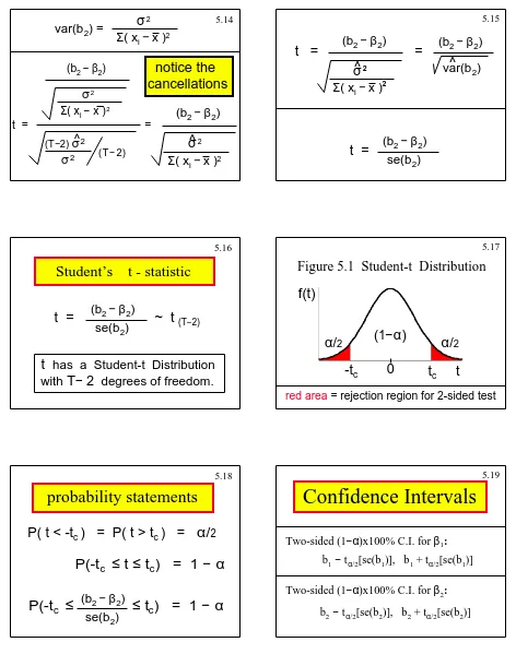
notice the

cancellations

(b

₂

− β

₂

)

σ

2

Σ

( x

_i

−

x )

2

^

t = =

(b

2

− β

2

)

var(b

^

₂

)

t =

(b

2

− β

2

)

se(b

₂

)

5.15

Student’s t - statistic

t = ~ t

(b

2

− β

2

)

_(T₋₂₎

se(b

₂

)

t

has a Student-t Distribution

with

T

−

2

degrees of freedom.

[image:25.612.70.542.100.699.2]

Figure 5.1 Student-t Distribution

(

1−α

)

t

0

f(t)

-t

_c

t

_c

α

/

2

α

/

2

red area

= rejection region for 2-sided test

5.17

probability statements

P(-t

_c

≤

t

≤

t

_c

) = 1

−

α

P( t < -t

_c

) = P( t > t

_c

) =

α/

2

P(-t

_c

≤

(b

2

− β

2

)

≤

t

_c

) = 1

−

α

se(b

₂

)

Confidence Intervals

Two-sided (1

−α

)x100% C.I. for

β

₁

:

b

₁

−

t

_α_/2

[se(b

₁

)], b

₁

+ t

_α_/2

[se(b

₁

)]

b

₂

−

t

_α_/2

[se(b

₂

)], b

₂

+ t

_α_/2

[se(b

₂

)]

Two-sided (1

−α

)x100% C.I. for

β

₂

:

(26)

25

Student-t vs. Normal Distribution

1. Both are symmetric bell-shaped distributions.

2. Student-t distribution has fatter tails than the normal.

3. Student-t converges to the normal for infinite sample.

4. Student-t conditional on degrees of freedom (df).

5. Normal is a good approximation of Student-t for the first few decimal places when df > 30 or so.

Hypothesis Tests

1. A null hypothesis, H

₀

.

2. An alternative hypothesis, H

₁

.

3. A test statistic.

4. A rejection region.

5.21

Rejection Rules

1. Two-Sided Test:

If the value of the test statistic falls in the critical region in either tail of the t-distribution, then we reject the null hypothesis in favor of the alternative.

2. Left-Tail Test:

If the value of the test statistic falls in the critical region which lies in the left tail of the t-distribution, then we reject the null hypothesis in favor of the alternative.

2. Right-Tail Test:

If the value of the test statistic falls in the critical region which lies in the right tail of the t-distribution, then we reject the null hypothesis in favor of the alternative.

Format for Hypothesis Testing

1. Determine null and alternative hypotheses. 2. Specify the test statistic and its distribution

as if the null hypothesis were true.

3. Select

α

and determine the rejection region. 4. Calculate the sample value of test statistic. 5. State your conclusion.

5.23

practical vs. statistical

significance in economics

Practically but not statistically significant:

When sample size is very small, a large average gap between the salaries of men and women might not be statistically significant.

Statistically but not practically significant:

When sample size is very large, a small correlation (say, ρ = 0.00000001) between the winning numbers in the PowerBall Lottery and the Dow-Jones Stock Market Index might be statistically significant.

Type I and Type II errors

Type I error:

We make the mistake of rejecting the null hypothesis when it is true.

α

= P(rejecting H₀ when it is true).

Type II error:

We make the mistake of failing to reject the null hypothesis when it is false.

(27)

26

Prediction Intervals

A (1

−α

)x100% prediction interval for y

_o

is:

y

_o

± t

_c

se( f )

^

se( f ) = var( f )

^

f = y

^

o

−

y

o

Σ(

x

_t

−

x

)

2

var( f ) =

^

σ

2

1 + +

1

Τ

(

x

o

−

x

)

2

^

The Simple Linear

Regression Model

Chapter 6

6.1

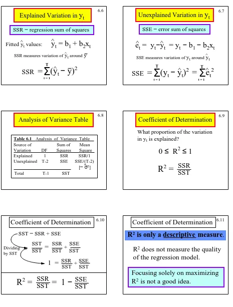
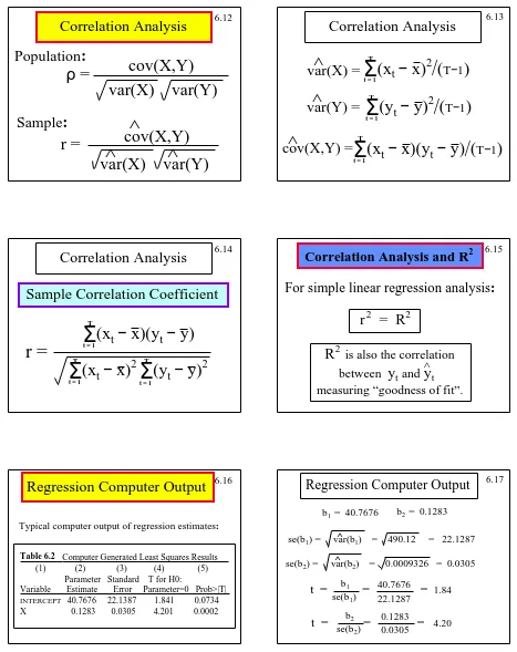
Explaining Variation in

y

t

Predicting y

_t

without any explanatory variables:

y

t

=

β

1

+ e

t

Σ

e

t

=

Σ

(y

t

−

β

1

)

2

t = 1 t = 1

T T

=

−2

Σ

(y

t

−

b

1

) = 0

∂Σ

e

2_t

t = 1

t = 1 T

T

∂

β

1

Σ

(y

t

−

b

1

) = 0

t = 1 T

Σ

y

t

−

Tb

1

= 0

t = 1 T

b

1

= y

Why not y?

Explaining Variation in

y

t

y

t

= b

1

+ b

2

x

t

+ e

^

t

Unexplained variation:

y

t

= b

1

+ b

2

x

t

^

Explained variation:

e

t

= y

t

−

y

^

t

= y

t

−

b

1

−

b

2

x

t

^

6.3

Explaining Variation in

y

t

y

t

= y

t

+ e

^

t

Why not y?

^

y

t

−

y = y

^

t

−

y + e

^

t

using y as baseline

SST = SSR + SSE

Σ

(y

t

−

y)

2

=

Σ

(y

t

−

y)

2

+

Σ

e

t

t = 1 T

^

T T

t = 1 t = 1

2 cross product

term drops

out

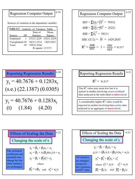
Total Variation in

y

t

SST = total sum of squares

SST measures variation of

y

t around

y

Σ

(y

t

−

y)

2

t = 1 T

SST

=

(28)

27

Explained Variation in

y

t

SSR = regression sum of squares

y

t

= b

1

+ b

2

x

t

^

Fitted y

^

t

values:

SSR measures variation of

y

^t around

y

Σ

(y

t

−

y)

2

t = 1 T

SSR

=

^

Unexplained Varia