www.elsevier.nl / locate / econbase
Does parents’ money matter?
* John Shea
Department of Economics, University of Maryland, College Park, MD 20742, USA
Abstract
This paper asks whether parents’ income per se has a positive impact on children’s abilities. Previous research has established that income is positively correlated across generations. This does not prove that parents’ money matters, however, since income is presumably correlated with ability. This paper estimates the impact of parents’ income by focusing on income variation due to factors – union, industry, and job loss – that arguably represent luck. I find that changes in parents’ income due to luck have a negligible impact on children’s human capital for most families, although parents’ money does matter for
families whose father has low education. 2000 Elsevier Science S.A. All rights
reserved.
Keywords: Social mobility; Human capital; Redistribution
JEL classification: H50; J62
1. Introduction
This paper asks whether parents’ income per se affects children’s abilities. In the absence of government intervention, we would expect children born to rich parents to acquire more human capital than children born to poor parents if capital markets are imperfect, in the sense that parents cannot pledge their children’s
*Tel.: 11-301-405-3491.
E-mail address: [email protected] (J. Shea)
future earnings as collateral when borrowing to invest in their children (Loury,
1
1981; Becker and Tomes, 1986; Mulligan, 1997). If parents’ money matters to children’s skills, then government intervention may be warranted on both equity and efficiency grounds (Galor and Zeira, 1993; Hoff and Lyon, 1995; Benabou, 1996). Concern over links between parental resources and children’s outcomes provides a rationale for programs that redistribute resources to low-income families or invest in children directly, such as public education, Medicaid, and the
2
Earned Income Tax Credit. The potential impact of parents’ income on children’s skills is also important to policy debates on school finance reform (Hoxby, 1996; Fernandez and Rogerson, 1998)) and college admission and scholarship rules (Clotfelter, 1999).
Empirically, a substantial body of research shows that economic status is persistent across generations: children raised in high-income families earn more than children raised in low-income families. Solon (1992) and Zimmerman (1992), for instance, find that the correlation between fathers’ and sons’ permanent earnings is near 0.4, while Corcoran et al. (1992), Hill and Duncan (1987) and others show that parents’ income remains important even after controlling for
3
parents’ education and other observable parental characteristics. While these studies are informative, they do not prove that parents’ money matters. High-earning parents presumably have more ability on average than low-High-earning parents. If ability is transmitted from parents to children through genes or culture, then incomes will be persistent across generations even if parents’ income per se doesn’t matter. Put differently, an ordinary least squares (OLS) regression of children’s income on parents’ income will yield an upward-biased estimate of the causal impact of parents’ income, due to a positive correlation between parents’ income and children’s ability. One can presumably reduce this bias by controlling for observable measures of parents’ ability. However, some bias will remain if part of ability is unmeasured.
Ideally, one would test whether parents’ money matters by dropping money on the doorsteps of randomly selected parents, then tracking the subsequent labor market performance of their children. In this paper, I attempt to approximate such a natural experiment by isolating observable determinants of parents’ income that arguably represent luck. I focus on variations in fathers’ labor earnings due to union status, industry, and involuntary job loss due to plant closings and other establishment deaths. Existing research (e.g. Lewis, 1986; Krueger and Summers,
1
Mayer (1997, Chapter 3) discusses at length competing theories of the link between parents’ resources and children’s outcomes, including sociology-based theories that emphasize the link between parental income and children’s formation of expectations.
2
Haveman and Wolfe (1995) calculate that total US public investment in children in 1992 amounted to $333 billion, or 5.4 percent of GDP.
3
1988) demonstrates that wages vary substantially with union and industry status, controlling for observable skills. Moreover, some economists contend that union and industry wage premia reflect rents rather than unobserved ability differences. If this interpretation is correct, then I can estimate the impact of parents’ income by comparing the children of union or high-wage industry fathers to the children of nonunion or low-wage industry fathers with similar observable skills. Similarly, Cochrane (1991), Jacobson et al. (1993) and others show that involuntary job loss has a large and persistent negative impact on earnings. If plant closings are exogenous with respect to employees’ unobservable skills, then I can estimate the impact of parents’ income by comparing the children of displaced fathers to the children of nondisplaced fathers with similar observable skills. Operationally, I draw a sample of children from the Panel Study of Income Dynamics (PSID), and perform two-stage least squares (2SLS) regressions of children’s income on demographic characteristics, fathers’ observable skills, and measures of parents’ income, using fathers’ union, industry and job loss variables as instruments for parents’ income.
My estimates of the impact of parents’ income could be upward biased for two reasons. First, luck may be correlated across generations. For instance, union fathers may be able to bequeath union jobs to their children. Second, my instruments may be correlated with unobserved ability; for instance, union fathers may be more able than nonunion fathers with similar observable skills. If unobserved ability is persistent across generations, then children of union fathers will fare better than children of nonunion fathers even if parents’ income per se doesn’t matter. I correct for the first bias in some specifications by removing the part of children’s income due to children’s observable luck and examining whether parents’ income affects children’s skill-related income. Unfortunately, I cannot correct for the second source of bias. My estimates thus arguably represent an upper bound for the true impact of parents’ income on children’s skills.
Given this caveat, it is perhaps surprising that on the whole my results suggest that parents’ money does not matter. For my full sample, I find that the impact of parents’ income on children’s human capital is positive, significant and econ-omically large when estimated using OLS, but insignificant and frequently negative using 2SLS. I find that union and industry status are persistent across generations, particularly for sons, so that removing the component of children’s income due to luck further reduces the estimated impact of parents’ income. While my 2SLS estimates are relatively imprecise, the difference between OLS and 2SLS estimates is frequently large enough to be statistically significant.
years of schooling; on the other hand, I find no evidence that the impact of parental income varies by the level of income per se.
While there are many existing studies that document the association between parents’ income and children’s outcomes, there are only a handful that attempt to overcome the endogeneity of parents’ income with respect to children’s ability; I
4
will critique these studies briefly here. Scarr and Weinberg (1978) examine the relationship between IQ and parental attributes in samples of biological adoles-cents and adolesadoles-cents who were adopted prior to their first birthday. They find a significant positive relationship between income and IQ among biological children, but no relationship among adopted children. The authors conclude that the apparent impact of income on IQ is due to genetic factors. A critic would note that the samples are small and homogenous (the adopted children, for instance, come from 104 affluent Minnesota families) and that income is measured for only one year, potentially biasing the impact of income downwards in both samples.
Blau (1999) examines the relationship between parents’ income and children’s test scores using the matched mother–child data from the National Longitudinal Survey of Youth (NLSY). Blau finds that income has a small positive effect on test scores in OLS regressions controlling for parental characteristics, but no effect in regressions controlling for child fixed effects, in which the impact of income is identified by comparing test results in years of high parental income to results for the same child in years of low income. A critic would note that Blau’s approach focuses attention on short-run variation in parents’ income, rather than cross-section variation in long-run income; the former type of variation could have less impact on children to the extent that parents can borrow and save, to the extent that income is measured with error, and to the extent that children’s outcomes
5
depend on lagged as well as current income.
Mayer (1997) uses several different approaches to identify the ‘true’ impact of
4
There are also several studies examining the impact of the Negative Income Tax experiments on children. Venti (1984) and Mallar (1977) find that the adolescent children of treatment families (i.e. families eligible for NIT benefits) complete more schooling and are less likely to work than the children of control families, while Maynard (1977) finds mixed evidence on the effects of treatment on test scores of younger children. The NIT evidence is not very informative about the impact of parents’ income on children, however, because NIT treatment families were subject to high marginal tax rates, which presumably had an independent effect on schooling, parenting and labor market decisions. For example, we would expect NIT treatments to increase adolescent schooling even if parents’ income per se is irrelevant to schooling, because high tax rates on current earnings reduce the opportunity cost of going to school.
5
6
parents’ income on children; I focus on two examples. First, Mayer examines the link between children’s outcomes and parents’ income from assets and child support payments, arguing that such income is less correlated with ability than labor earnings or transfer payments. Mayer finds that such income has a smaller impact than overall income on children’s test scores, teenage childbearing, dropping out of school, and single motherhood, but a similar positive and significant effect on children’s years of schooling, wages, and earnings, suggesting that asset income and child support payments may be positively correlated with
7
unobserved parental ability. Second, Mayer examines the impact of state welfare benefit differences. She finds that children of both married-parent and single-parent families fare better in high-benefit states, suggesting that states with stronger labor markets pay higher benefits. However, the gap between children of married and single parents does not narrow as benefits increase, suggesting that benefit levels per se do not matter for children. On the other hand, Mayer does not establish that higher benefits narrow the gap in parental resources between single and married parents. Such narrowing is not automatic, as Mayer points out, because higher welfare benefits are typically offset by lower food stamp benefits; because not all single parents go on welfare; and because higher welfare benefits may induce labor force withdrawal by single mothers. Mayer’s results could therefore be due either to a small ‘second-stage’ effect of income on children, or to a small ‘first-stage’ effect of benefits on income.
Duflo (1999) is perhaps the closest in spirit to this paper. She uses the unexpected expansion of eligibility for old age pensions to South African blacks in the early 1990s to examine the impact of grandparents’ resources on child health. By comparing outcomes across groups of children differentially affected by the program expansion (children with living grandparents versus children without,
6
Mayer takes two other approaches to estimating the true impact of parents’ income. First, she compares the impact on children’s outcomes of recent income to the impact of income received after the outcome is observed, and typically finds stronger effects of future income than one would expect merely based on the correlation between current and future income. Since future income per se should not influence children’s outcomes, Mayer argues that most of the apparent impact of parents’ income must be due to unobserved heterogeneity. I find this argument unconvincing for two reasons: (1) Mayer estimates ‘recent’ income using only a 5-year window, so that future income may appear to matter because it is correlated with income received prior to the 5-year window, which may affect children’s outcomes; (2) anticipated future income should affect current spending on children if households can borrow and save. Second, Mayer examines trends over time in the distribution of parents’ income and finds that they are not reflected in trends of the distribution of children’s outcomes. This evidence is interesting but may be confounded by trends in other variables such as social mores, drug use, and wages for low-skilled workers.
7
black children versus white children whose grandparents were already eligible, and so on), Duflo shows that pension availability had a positive impact on children’s weight and height. Note that Duflo’s results are not necessarily inconsistent with mine, since the impact of parental resources on children may be higher in developing countries than in the contemporary US, where public investments in schooling and child health are relatively high.
The rest of this paper proceeds as follows. Section 2 presents a simple model of intergenerational transmission. The model illustrates why OLS estimates are likely to overstate the true impact of income on children, shows how one can estimate the true impact using instrumental variables, and discusses possible biases arising from this approach. Section 3 describes the data, and Section 4 presents empirical results. Section 5 concludes.
2. A simple model of intergenerational transmission
This section presents a simple, mechanical model of intergenerational
transmis-8
sion, designed to fix ideas and to motivate the empirical work below. Assume that we observe permanent income for a sample of parents and children. Assume that a child’s income (Y ) depends on two unobservables: human capital (H ) and lucki i
(L ):i
Yi5Hi1Li (1)
where for our purposes, H could encompass factors such as innate intelligence,i
manual dexterity, education, and work ethic. Assume that children’s human capital depends stochastically on both parents’ human capital and parents’ income:
Hi5rHi211gYi211´i (2)
where´i is a disturbance term assumed orthogonal to parental attributes. The first term on the right hand side of (2) represents the transmission of ability from parents to children through genes and culture. The second term represents the causal impact of parents’ income on children’s human capital. My goal in this paper is to estimate g.
Combining (1) and (2) we have
Yi5gYi211rHi211Li1´i (3)
Now suppose we regress Y on Yi i21 using OLS. The resulting estimate of g is
8
upward biased, since parents’ income Yi21 is positively correlated with parents’ human capital Hi21.
Now suppose, however, that there exists a vector of observable variables, Xi21, that may reflect either parental skill or luck, and a vector of observables, Zi21, that conditional on Xi21 reflect only parental luck. In the empirical work below, Xi21
includes variables such as fathers’ education and occupation, while Zi21 includes fathers’ union, industry, and job loss variables. Assume these variables are related to human capital and luck as follows:
H
Hi215a1Xi211ui21 (4)
L
Li215b1Xi211b2Zi211ui21 (5)
The key assumption in Eqs. (4) and (5) is that the component of Zi21 orthogonal
H
to Xi21is itself orthogonal to ui21, so that setting the coefficients of Zi21 in (4) to zero is a valid exclusion restriction. In my application, this amounts to assuming that, conditioning on observable skills, fathers’ union, industry and job loss experience are orthogonal to the part of unobserved ability transmitted across generations. This assumption will be valid if variation in union, industry and displacement status (controlling for observable skills) is due solely to luck.
Substituting (4) into (3), we have
H
Yi5gYi211lXi211rui211Li1´i (6)
where l 5 ra1. Under the assumptions made above, we can now estimate g consistently by regressing Y on Yi i21and Xi21, using Zi21and Xi21as instruments. Intuitively, this procedure identifies g by comparing the children of union (or high-wage industry, or nondisplaced) fathers to the children of nonunion (or low-wage industry, or displaced) fathers with otherwise similar observable characteristics.
There two obvious reasons why this procedure might produce biased estimates ofg. First, luck may be correlated across generations. For example, if union jobs pay rents, then there are presumably non-market mechanisms allocating union jobs to the lucky few. If these mechanisms include social connections or nepotism, then children of union fathers should have an edge obtaining union jobs. In this case, Zi21 would be correlated with L via Z , and IV estimates ofi i g would be biased upwards. Below, I counteract this bias by removing the component of children’s income due to children’s luck (Z ) and examining the relationship between parents’i
H
generations, then Zi21would be correlated with ui21, and IV estimates ofg would again be biased upwards. It seems unlikely that unobserved ability would be correlated with job loss due to establishment death. There is a theoretical presumption, however, that union and high-wage industry workers are more able, since jobs that pay rents should attract an excess supply of willing workers, affording firms the luxury of selecting the best applicants (Pettengill, 1979).
Empirically, the strongest evidence for the unobserved ability view comes from studies using panel data (Murphy and Topel, 1990; Jakubson, 1991). These studies find that union and industry switchers experience wage changes that are small relative to the corresponding cross-section wage differences, suggesting that union and industry premia are primarily due to differences in unobserved ability. Other studies, however, counter that spurious union and industry switches in panel data are common relative to true switches, biasing panel estimates of union and industry premia downward (Freeman, 1984). Furthermore, studies that attempt to reduce the impact of measurement error find wage changes for switchers that are similar to cross-section wage differences (Chowdhury and Nickell, 1985; Krueger and Summers, 1988; Gibbons and Katz, 1992). Additional evidence is provided by Holzer et al. (1991), who find that union wage premia generate a significant increase in the number of applications per job opening, while industry wage premia have a smaller and insignificant effect on job queues. Since jobs paying rents should attract excess applicants, this evidence suggests that union premia may be more plausibly interpreted as rents than industry premia.
In this paper, I make an identifying assumption that my instruments are uncorrelated with unobserved ability. I concede, however, that union and industry premia may be partly due to ability, in which case my estimates ofg arguably are an upper bound for the true impact of parents’ income on children’s human capital.
3. Data
1968; (4) there is at least 1 year between 1968 and 1989 in which the child is less than 23 and in which the father is a household head, aged 25–64, with positive hours and earnings; and (5) information on education, occupation and industry are available for both father and child. My sample consists of 3033 children (1475 sons and 1558 daughters) matched to 1271 fathers; of these, 1669 children and 783 fathers are from the representative subsample. My sample composition differs from Solon (1992) in that I allow multiple children from the same family and daughters as well as sons. In my empirical work, I allow disturbances to be correlated among children from the same family, and I examine both pooled results and results treating sons and daughters separately.
My empirical strategy requires that I measure the permanent income of parents and the human capital of children. For parents, I use two measures of income: fathers’ labor earnings and parents’ total income, consisting of labor earnings,
9
asset income and transfer income of head and spouse. For children, I measure
10
human capital using wages, labor earnings, total income, and years of schooling. Income, earnings and wages are expressed in 1988 dollars. I average fathers’ earnings and parents’ income over all years in which the father is a household head aged 25–64, and in which the child is less than 23 years old and thus potentially still dependent on parental support. For children, I average wages and earnings over all years in which the child is a household head or spouse aged 25 or
11
older. I compute average earnings including years of zero earnings, and compute average wages weighting by annual hours worked; results are similar if I exclude
9
I measure parents’ total income in year T as labor, transfer and asset income of the 1968 father in year T plus labor, transfer and asset income of the 1968 spouse (if any) in year T, regardless of whether the head and spouse are still living in the same household in year T. In years when asset and transfer income are only available for the head and spouse combined, I compute income for each parent by dividing reported combined income by the number of primary adults in the parent’s household (which is always either one or two). My measure of asset income equals asset income reported in the PSID plus an imputed income stream equal to 7 percent of reported housing equity; results are not sensitive to the inclusion of imputed housing income or to the assumed rate of return. I also experimented with measures of parental resources that include both income and wealth, where I measure wealth as housing equity plus asset wealth, imputing the latter using PSID asset income and time series data on rates of return. The OLS results using this broader measure of resources were somewhat weaker than those using income alone, which is perhaps not surprising given likely measurement error in my measure of nonhousing wealth; the 2SLS results were qualitatively similar to those reported in the paper.
10
When available, I measure the nominal wage as the reported straight time hourly wage; otherwise, I measure the nominal wage as annual labor earnings divided by annual hours. I convert earnings, income and wages reported in year t to 1988 dollars using the Consumer Price Index for year t21.
11
years of zero earnings. I average wages, earnings and income over many years to obtain the most accurate possible measure of permanent income; Solon (1992) and Zimmerman (1992) show that measurement error in parents’ permanent income biases estimated intergenerational income correlations downwards, and that averaging over several years attenuates this bias. To correct for the fact that I observe parents and children at different points of the life cycle, my regressions include a constant and sample averages of fathers’ and children’s age and age
12 ,13
squared; I also include dummy variables for race and gender.
I also require observable measures of parents’ ability and luck. The vector Xi21
includes fathers’ years of schooling and fathers’ sample averages of one-digit occupational dummies, a marriage dummy, an SMSA dummy and a South
14 ,15
dummy; results are similar if I also include mothers’ education. The vector Zi21consists of the sample average of a dummy for fathers’ union status; fathers’ average industry wage premium, estimated by combining fathers’ reported industry with estimates of industry wage premia in Krueger and Summers (1988); and an indicator for whether the father ever reports losing a job because the company folded, changed hands, moved out of town, or went out of
12
One could argue that removing life-cycle variation from parental income is unnecessary in my context; if parents’ income per se matters for children’s success, then children born to older parents should tend to do better than children born to younger parents. As a practical matter, however, I must remove such variation from my data because sample attrition and truncation of the data in 1968 imply cross-sectional differences in the extent to which I observe parents’ complete life-cycle histories. For instance, I would not want to conclude that father A has higher lifetime earnings than father B simply because father A was 40 in 1968 with a 17-year old child while father B was 25 in 1968 with a 2-year old child.
13
I experimented with replacing the constant term with a vector of period variables indicating the fraction of sample years spent in different time periods; this formulation corrects for business cycle and secular variation in income. Adding these period variables made little difference to the results. I also experimented with interacting children’s age and age squared with gender, with little effect on the results.
14
In most cases, fathers’ years of schooling is taken from the 1968 PSID individual file. If fathers’ years of schooling is reported as a 0 or a 99 in 1968, I use categorical education data from 1968 through 1972 to impute fathers’ years of schooling. I estimate children’s years of education as of the first year in which they are eligible for sample inclusion; from 1976 through 1984 and 1991 through 1992, this is taken from family-level data, while between 1985 and 1990 this is taken from individual-level data. If children’s reported education is 0 or 99, I use data from surrounding years to impute schooling. I dropped cases in which I was unable to impute years of schooling from my sample.
15
16 ,17 ,18
business. I use the industry premium rather than industry dummy variables to minimize the risk of small-sample 2SLS bias due to first-stage overfitting, although in practice 2SLS estimates ofg using eight one-digit industry dummies instead of the industry premium are only slightly higher than the estimates reported in this paper.
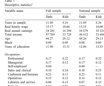
Table 1 presents descriptive statistics for fathers and children, for both the full sample and the representative (‘National’) and poverty subsamples; here and below, I omit sampling weights when examining the representative and poverty subsamples separately. For all variables, I report the mean across sample members
19
of individual averages over time. Thus, for instance, the reported SMSA statistic for fathers could imply that 66 percent of fathers live in a city all the time, or that all fathers live in a city 66 percent of the time; the first case is closer to the truth in this and similar instances. On average, I have almost 12 years of data per father and over 8 years of data per child in the full sample, implying that I measure
16
The PSID did not ask union questions in 1973; I compute fathers’ average union status using only data from years other than 1973. In later years, the PSID asked both whether one’s job is covered by a union contract and whether one belongs to a labor union; I use the contract question to define union status.
17
I impute wage premia at the two-digit industry level, using estimates reported in Table 2 of Krueger and Summers (1988). I use the reported results from the 1974 May CPS for sample years prior to 1977; I use results from the 1979 CPS for sample years 1977–1981; and I use results from the 1984 CPS for all sample years after 1981. Prior to 1981, the PSID industry classification system is more aggregated for some industries than the classification used by Krueger and Summers; for these years, I average Krueger and Summers’ estimated premia for disaggregated industries, weighting by the share of sample fathers in each disaggregated industry in 1981. Krueger and Summers do not report wage premia for workers in agriculture or government; I estimate premia for these industries in the PSID, regressing sample fathers’ average wages on demographics, fathers’ skills, and sample averages of one-digit industry dummy variables. The PSID did not ask industry questions until 1971; I define industry premia averaging only sample years from 1971 on. As with occupation, some individuals do not report a valid industry in some years; for these individuals, industry premia are defined as averages over all sample years for which some industry is reported. If an individual is unemployed or retired in a given interview, I use industry on the previous job when available.
18
Notice that my job loss indicator equals one if a father ever reports a job loss due to establishment death; unlike other sample variables, I do not measure this indicator year by year and then divide by each individual’s total sample years. I measure job loss as a zero-one indicator rather than a sample average because I found that the former variable had more explanatory power in average earnings and wage regressions than the latter, which is reasonable if job loss due to establishment death has long-run consequences for earnings and wages. I also experimented with interacting job loss with the fraction of sample years occurring after the job loss, with little impact on the results.
19
Table 1
a
Descriptive statistics
Variable name Full sample National sample Poverty sample
Dads Kids Dads Kids Dads Kids
Years in sample 11.80 8.16 11.89 8.26 10.95 7.48
Real hourly wage 15.17 10.04 15.35 10.00 9.55 8.14
Real annual earnings 34 201 18 294 34 879 18 324 19 168 13 785 Total income 47 789 33 729 48 612 33 686 27 568 23 745
Age 44.27 29.12 44.26 29.13 44.06 29.02
Black 0.09 0.09 0.08 0.09 0.63 0.64
Years of education 11.90 13.31 12.06 13.33 8.84 12.60
Occupation:
Professional 0.17 0.22 0.17 0.22 0.05 0.12
Managerial 0.17 0.12 0.17 0.12 0.05 0.07
Self-employed 0.04 – 0.04 – 0.05 –
Sales and clerical 0.10 0.24 0.10 0.23 0.06 0.23
Craftsmen and foremen 0.23 0.11 0.23 0.11 0.22 0.11
Operatives 0.15 0.12 0.16 0.12 0.25 0.19
Laborers and service 0.08 0.15 0.07 0.15 0.26 0.24
Farmers 0.04 0.01 0.05 0.01 0.03 0.00
Protective service 0.02 0.03 0.02 0.03 0.03 0.04
Living in SMSA 0.66 0.55 0.62 0.53 0.73 0.65
Living in the south 0.27 0.30 0.28 0.30 0.64 0.65
Married 0.92 0.68 0.92 0.69 0.88 0.57
Union 0.31 0.12 0.30 0.13 0.30 0.13
Industry premium 0.03 0.00 0.04 0.00 0.03 20.01
Job loss 0.16 0.10 0.15 0.10 0.20 0.12
a
This table presents sample means of the variables used in the paper, for both the full sample and the nationally representative (‘National’) and poverty subsamples. The numbers reported are averages across sample members of individual means over time; thus, for instance, the numbers are consistent with either 28 percent of sample fathers living in the South for the entire sample, or with all fathers living in the South 28 percent of the time. The first scenario is closer to the truth in this and similar instances. See the text for further information.
permanent incomes over a reasonably long time span for the typical observation. Note that the representative sample appears similar to the full sample, while poverty sample observations have lower income and lower education, as well as a greater likelihood of being black, living in the South, and working in a blue collar occupation.
Table 2
Industry premium 1.156 0.878 1.293 0.833
(0.162)* (0.145)* (0.319)* (0.138)*
Job loss 20.099 20.090 20.026 20.073
(0.034)* (0.042)* (0.053) (0.033)*
F statistic 104.3 45.02 71.90 61.29
[0.000] [0.000] [0.000] [0.000]
Wald statistic 250.5 157.6 432.8 85.25
[0.000] [0.000] [0.000] [0.000]
Partial R-squared 0.097 0.076 0.139 0.075
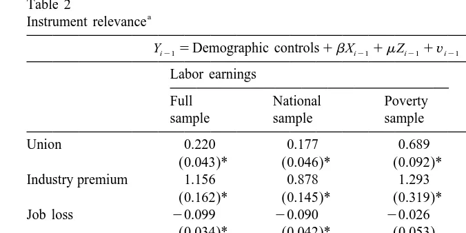
a
This table presents results from the first-stage regressions of fathers’ log average earnings and parents’ log average income on demographic variables and observable measures of fathers’ skill and luck, using the full sample as well as the nationally representative (‘National’) and poverty subsamples of the PSID. The first three rows report coefficients on three measures of fathers’ luck, with robust standard errors in parentheses; * denotes significance at 5 percent. The fourth and fifth rows report the results of a standard F-test and a robust Wald test of the null hypothesis that the coefficients on fathers’ luck variables are jointly zero, with p-values in brackets. The final row reports the R-squared from regressing the component of Y orthogonal to demographic and skill controls on the component of fitted
Y orthogonal to demographics and skill controls.
parentheses and are robust to heteroscedasticity of unknown form as well as
20 ,21
arbitrary error covariance within families. For the complete sample and for both subsamples, the results indicate that belonging to a union or a high-wage industry has a positive and significant effect on fathers’ earnings. Job loss has a negative and significant effect on earnings in the full and representative samples, but is insignificant in the poverty sample. For the full sample, all three variables
20
For the OLS regressions reported in this paper, standard errors are computed as follows. Let the J families in the sample be indexed by j. Let X denote the matrix of RHS variables for family j; thisj
*
matrix has dimension T k, where T is the number of children for family j and k is the number of RHSj j
*
variables. Finally, let e denote the T 1 vector of estimated disturbances for family j. Then thej j
estimated variance–covariance matrix is:
For 2SLS regressions, standard errors are computed in the same way, with X replaced by X, the projection of X on the instruments.
21
have a significant effect on total income, but the impacts are smaller for income than for earnings. These instruments are highly significant; in all cases, conven-tional F-tests and Wald tests (robust to nonspherical disturbances) easily reject the null hypothesis of joint insignificance of Z at one percent. The final row reports the partial R-squared, equal to the squared correlation between the components of fitted and actual income orthogonal to demographic variables and observable skills. For the full sample, the partial R-squared is 0.097 for earnings and 0.075 for income, suggesting that my instruments capture more cross-section variation in earnings than income. Note, too, that the instruments capture more variation in the poverty sample than in the representative sample.
4. Empirical results
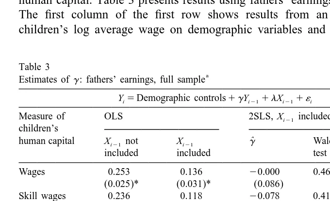
This section presents estimates of the impact of parents’ income on children’s human capital. Table 3 presents results using fathers’ earnings for the full sample. The first column of the first row shows results from an OLS regression of children’s log average wage on demographic variables and fathers’ log average
Table 3
a
Estimates ofg: fathers’ earnings, full sample
Yi5Demographic controls1gYi211lXi211´i
Measure of OLS 2SLS, Xi21 included
children’s
ˆ
human capital Xi21not Xi21 g Wald Hausman
included included test test
Wages 0.253 0.136 20.000 0.46 0.10
(0.025)* (0.031)* (0.086)
Skill wages 0.236 0.118 20.078 0.41 0.01
(0.022)* (0.026)* (0.082)
Earnings 0.356 0.206 20.028 0.95 0.15
(0.043)* (0.055)* (0.167)
Skill earnings 0.324 0.171 20.173 0.74 0.03
(0.041)* (0.051)* (0.159)
Total income 0.276 0.211 0.076 0.98 0.16
(0.026)* (0.034)* (0.098)
Skill income 0.244 0.176 20.069 0.97 0.01
(0.025)* (0.031)* (0.104)
Education 1.225 0.373 20.063 0.99 0.21
(0.011)* (0.113)* (0.354)
a
earnings, with robust standard errors in parentheses. The estimated effect of fathers’ earnings is 0.253 and is significantly different from zero.
The second column of the first row presents OLS estimates of g from the specification
Yi5Demographic variables1gYi211lXi211´i (7)
where Y is the child’s log wage, Yi i21 is fathers’ log earnings, and Xi21 includes measures of fathers’ education, occupation, region, marital status and urbanicity. When I control for fathers’ observable skills, the estimate ofg remains statistically significant, but falls to 0.136, suggesting that the estimate in the first column is biased upward by a positive correlation between fathers’ earnings and abilities that are transmitted across generations.
While controlling for observable skills presumably reduces the upward bias ing, some bias is likely to remain if there are important unobserved differences in ability among fathers. Accordingly, the third column presents 2SLS estimates of (7) instrumenting for Yi21 using Zi21, consisting of fathers’ union, industry and job loss variables. Instrumenting for fathers’ earnings reduces the point estimate of g from 0.136 to zero. The final two columns of the first row present the p-values of two specification tests: a test of overidentifying restrictions, computed by regressing the estimated 2SLS residuals on demographics, Xi21, and Zi21, then performing a Wald test (using the robust variance–covariance matrix) of the hypothesis that the coefficients on all variables are zero; and a Hausman test of the exogeneity of fathers’ earnings in Eq. (7), computed by testing the hypothesis that
22
the OLS and 2SLS estimates of g controlling for Xi21 are identical. I cannot reject the overidentifying restrictions, while I can reject exogeneity at 10 percent. Recall that 2SLS estimates ofg may still be upward biased if luck is correlated across generations; for instance, if children of union fathers have an edge getting union jobs themselves, they may fare well even if parents’ income per se is irrelevant. The second row of Table 3 accordingly examines the impact of fathers’ earnings on the component of children’s wages due to skill. To estimate this component, I first regress children’s log average wage (Y ) on demographici
variables, children’s observable skills (X ), and children’s observable luck (Z ). Ii i
then set the ‘skill wage’ equal to the actual wage minus the component of the fitted wage due to Z . From Table 3, removing the part of children’s wages due toi
observable luck has little impact on the OLS estimates ofg, but reduces the 2SLS estimate to 20.078; the difference between OLS and 2SLS is now significant at 1 percent.
22
Since the disturbance term in (7) is nonspherical, the formula for computing the variance of
gOLS2g2SLSgiven in Hausman (1978) does not apply, since OLS is not the most efficient estimator ofg
Table 4
a
Does luck persist across generations?
Zi5a 1 bZi211ui
Measure Sample of luck
All Boys Girls
children only only
Union 0.082 0.146 0.018
(0.017)* (0.027)* (0.018)
Industry 0.061 0.104 0.039
(0.029)* (0.039)* (0.036) Job loss 20.026 20.044 20.008
(0.015) (0.022)* (0.022)
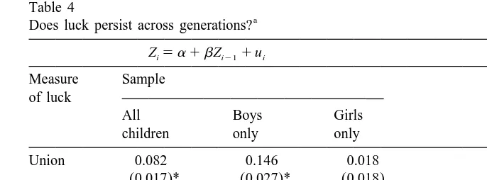
a
This table presents estimates of the impact of fathers’ union, industry and job loss status on children’s union, industry and job loss status. Robust standard errors are in parentheses; * denotes estimates that are significantly different from zero at 5 percent.
The last result suggests that labor market luck is correlated across generations. I present direct evidence on this conjecture in Table 4, which contains results from regressing children’s union, industry and job loss variables (Z ) on the corre-i
sponding fathers’ luck variables Zi21. The regressions are estimated using OLS;
23
probit estimation yielded qualitatively similar results. The results for all children suggest that union and industry premia are significantly and positively correlated across generations, while the incidence of job loss is insignificantly negatively correlated across generations. When I split the sample by gender, I find that union and industry premia are persistent only for boys. Fathers apparently bequeath their union and industry premia to their sons, but not to their daughters; I explore the consequences of this gender difference below.
The third and fourth rows of Table 3 present evidence for children’s labor earnings. The OLS estimate of g controlling only for demographics is 0.356, broadly consistent with Solon (1992), who estimates g to be near 0.4 in specifications involving fathers’ and sons’ earnings. The OLS estimate falls to 0.206 when I control for fathers’ observable skills, but remains highly significant. Instrumenting for fathers’ earnings, however, reduces estimatedg to 20.028, and removing the part of children’s earnings due to luck reduces g even further, to 20.173. The earnings estimates are less precise than the wage estimates; nevertheless, the difference between OLS and 2SLS is large enough to be significant at 3 percent for skill earnings.
The next two rows of Table 3 present results for children’s total income,
23
including labor, transfer and asset income of both the child and spouse. I define ‘skill income’ by removing only the luck component of the child’s labor earnings; I do not adjust spouse’s earnings or any transfer or asset income. The OLS estimates of g controlling for Xi21 are positive, significant, and comparable to estimates using children’s earnings alone. The 2SLS estimate for total income is positive, but small and insignificant; removing the component of children’s earnings due to luck reduces the 2SLS estimate to 20.069, which is significantly different from OLS at 5 percent.
The final row presents estimates using children’s years of schooling. When I use OLS and condition only on demographics, I find a strong positive relationship between fathers’ earnings and children’s schooling; the estimate suggests that doubling earnings would produce over a year of extra schooling per child. When I control for fathers’ observable skills but continue to use OLS, the response of children’s education to earnings declines but remains positive and significant. When I instrument for earnings, however, the estimate of g becomes negative, although not significantly different from OLS.
Table 5 presents results using parents’ total income. The point estimates are broadly similar to estimates using fathers’ earnings: the OLS estimates are positive and significant, while the 2SLS estimates are negative in most cases. The 2SLS
Table 5
a
Estimates ofg: parents’ income, full sample
Yi5Demographic controls1gYi211lXi211´i
Measure of OLS 2SLS, Xi21 included
children’s
ˆ
human capital Xi21not Xi21 g Wald Hausman
included included test test
Wages 0.340 0.199 0.050 0.47 0.27
(0.023)* (0.030)* (0.138)
Skill wages 0.320 0.170 20.066 0.26 0.06
(0.021)* (0.029)* (0.132)
Earnings 0.467 0.284 20.028 0.94 0.23
(0.050)* (0.066)* (0.263)
Skill earnings 0.427 0.227 20.247 0.68 0.05
(0.050)* (0.065)* (0.253)
Total income 0.367 0.297 0.114 0.97 0.24
(0.031)* (0.043)* (0.157)
Skill income 0.327 0.240 20.104 0.97 0.03
(0.032)* (0.047)* (0.165)
Education 1.859 0.856 20.060 0.98 0.09
(0.101)* (0.139)* (0.565)
a
estimates are less precise than those in Table 3, reflecting the fact that my instruments are less relevant for parents’ income than for fathers’ earnings. Nevertheless, the 2SLS estimates differ significantly from OLS at 5 percent for skill earnings and skill income, and at 10 percent for skill wages and years of schooling. Because earnings estimates are more precise, I focus on fathers’ earnings for the rest of the paper; results using parents’ income are broadly similar and are available from the author.
4.1. Each instrument separately
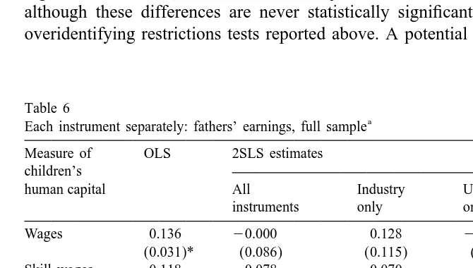
The 2SLS results reported to this point use all instruments simultaneously. Table 6 reports results using industry, union and job loss separately as instruments. In these experiments, I reassign variables excluded from the instrument vector Zi21
to the vector of observable skills Xi21. The results are broadly robust to the choice of instruments; the 2SLS estimates ofg lie below the corresponding OLS estimate in all but two cases, and are usually negative. The industry premium generates higher estimates ofg than the union and job loss variables in five of seven cases, although these differences are never statistically significant, consistent with the overidentifying restrictions tests reported above. A potential explanation for these
Table 6
a
Each instrument separately: fathers’ earnings, full sample Measure of OLS 2SLS estimates children’s
human capital All Industry Union Job Loss
instruments only only only
Wages 0.136 20.000 0.128 20.211 20.067
(0.031)* (0.086) (0.115) (0.175) (0.308)
Skill wages 0.118 20.078 0.070 20.300 20.060
(0.026)* (0.082) (0.113) (0.180) (0.307)
Earnings 0.206 20.028 20.050 20.082 0.344
(0.055)* (0.167) (0.216) (0.343) (0.656) Skill earnings 0.171 20.173 20.224 20.253 0.516
(0.051)* (0.159) (0.209) (0.329) (0.609)
Total income 0.211 0.076 0.086 0.092 20.059
(0.034)* (0.098) (0.134) (0.199) (0.393) Skill income 0.176 20.069 20.031 20.067 20.051
(0.031)* (0.104) (0.137) (0.211) (0.392)
Education 0.373 20.063 0.054 20.225 20.241
(0.113)* (0.354) (0.495) (0.727) (1.280)
a
differences is that industry is less exogenous with respect to unobserved ability than union status and job loss. This interpretation is consistent with the results of Holzer et al. (1991), discussed above. It is also consistent with prior logic: it would not be surprising to find that union jobs pay rents, since generating rents is a primary goal of unions; on the other hand, it is harder to explain why some industries would persistently pay rents relative to others.
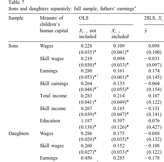
4.2. Sons and daughters separately
The specifications reported above pool sons and daughters. However, it is possible that parents’ income affects boys and girls differently. Accordingly, in Table 7, I estimate Eq. (7) allowing all coefficients to differ by gender. Results are as follows. First, the OLS estimates ofgare positive in all cases, and significant in all but one case. The OLS estimates are higher for girls than for boys in five of seven cases, although these differences are significant at 5 percent only for earnings and skill earnings. Second, the 2SLS estimates of g lie below the corresponding OLS estimates in all but one case, and are negative in most cases. The 2SLS estimates are lower for girls than for boys in all but one case, although these differences are not significant. Third, the differences between OLS and 2SLS estimates are less likely to be significant than in the pooled regressions, due to smaller sample sizes; nevertheless, the OLS and 2SLS estimates differ sig-nificantly at 5 percent in three cases, and at 10 percent in two addidtional cases. Fourth, removing the component of children’s income due to luck makes a larger difference for sons than for daughters. This is consistent with the evidence presented above that union and industry premia are significantly correlated across generations for sons but not daughters. Overall, the finding that parents’ income has little impact on children’s abilities seems to be robust to disaggregating by gender.
4.3. Are these estimates biased downwards?
Taken literally, most of the 2SLS estimates suggest that parents’ income is inconsequential or even detrimental to children’s skills. Above, I asserted that these estimates are likely if anything to be biased upwards, due to positive correlation between wage premia and unobservable ability transmitted across generations. Given my results, one might wonder if my 2SLS estimates ofg could instead be biased downwards. Here I discuss four possible sources of downward bias.
Table 7
a
Sons and daughters separately: full sample, fathers’ earnings
Sample Measure of OLS 2SLS, Xi21included children’s
ˆ
human capital Xi21not Xi21 g Wald Hausman
included included test test
Sons Wages 0.228 0.109 0.098 0.01 0.91
(0.035)* (0.041)* (0.100)
Skill wages 0.219 0.094 20.031 0.09 0.18 (0.030)* (0.033)* (0.097)
Earnings 0.280 0.161 0.174 0.96 0.94
†
(0.053)* (0.061)* (0.145)
Skill earnings 0.264 0.133 20.064 0.96 0.19
†
(0.048)* (0.055)* (0.154)
Total income 0.283 0.214 0.107 0.33 0.38
(0.041)* (0.049)* (0.122)
Skill income 0.267 0.185 20.131 0.87 0.02 (0.039)* (0.047)* (0.141)
Education 1.187 0.397 0.076 0.95 0.45
(0.138)* (0.126)* (0.427)
Daughters Wages 0.286 0.175 20.088 0.20 0.04
(0.029)* (0.035)* (0.132)
Skill wages 0.260 0.152 20.108 0.11 0.03 (0.027)* (0.033)* (0.122)
Earnings 0.450 0.285 20.178 0.96 0.10
†
(0.062)* (0.080)* (0.297)
Skill earnings 0.400 0.241 20.220 0.92 0.08
†
(0.061)* (0.077)* (0.272)
Total income 0.265 0.208 0.018 0.81 0.19
(0.032)* (0.039)* (0.148)
Skill income 0.215 0.164 20.024 0.91 0.21 (0.032)* (0.038)* (0.151)
Education 1.269 0.341 20.295 0.96 0.19
(0.124)* (0.177) (0.493)
a
This table presents estimates of the impact of fathers’ earnings the human capital accumulation of children, allowing coefficients to differ by child’s gender. Robust standard errors are in parentheses;
†
* denotes estimates significantly different from zero at five percent, while denotes estimates that differ significantly by gender at five percent. The final two columns present the p-values from a Wald test of overidentifying restrictions and a Hausman test of the null hypothesis of exogeneity of fathers’ earnings.
counteract the benefits of extra income; income variation due to labor market luck may generate lower estimates of g than variation due to dropping money on doorsteps.
supply. Existing research suggests that the intertemporal elasticity of labor supply for married men is low (Pencavel (1986)), and the long-run elasticity is presumably even smaller. In my sample, when I regress fathers’ log average hours on demographics, skills, and log average wages, I estimate a coefficient (standard error) on wages of 0.027 (0.042) using OLS, and 0.104 (0.077) using industry, union and job loss as instruments for wages; the long-run labor supply elasticity appears to be quite low in my sample. Labor supply may be more elastic for married women than for married men (Killingsworth and Heckman, 1986), suggesting that labor market opportunities and time spent with children may be more negatively correlated for mothers than for fathers. This is the main reason I use only fathers’ luck to identify the impact of parents’ income.
Second, my estimates of g could be biased downward if union or industry premia reflect compensating differentials rather than rents or unobserved ability. If wage premia compensate for low fringe benefits, then measured income differ-ences due to union and industry will overstate true differdiffer-ences in family resources, biasing estimatedg downward. If wage premia are instead compensation for poor working conditions, the implications for intergenerational transmission are am-biguous. If families treat all sources of income identically, then wage premia due to poor working conditions should enable liquidity constrained parents to raise their children’s skills, and my estimates of g should be unaffected. On the other hand, families may rationally decide to allocate rewards for poor working conditions to the worker’s consumption bundle; a father who has to work in unpleasant conditions may feel entitled to spend his compensating differential on a new boat rather than on his son’s education. In this case, measured income differences due to union and industry will again overstate cross-family differences in resources available to children, biasing my estimates ofg downward.
Empirically, there is little evidence that union and industry premia reflect compensating differences. Freeman and Medoff (1984) report that union workers express more concern with job safety than nonunion workers, but that actual workplace hazards are similar for union and nonunion jobs. Meanwhile, both Freeman and Medoff (1984) and Lewis (1986) cite evidence that union status has, if anything, an even larger impact on fringe benefits than on earnings. Similarly, Krueger and Summers (1988) find that fringe benefits reinforce rather than counteract industry wage differences, and that controlling for working conditions has little effect on industry premia. Overall, it seems unlikely that my estimates are
24
biased by compensating differentials.
Third, fathers’ labor market luck may be negatively correlated with the return to human capital investment in children. My estimation strategy assumes that the
24
optimal level of investment is independent of the child’s expected union and industry status. This may not be true. Lewis (1986), for instance, notes that the union wage premium is higher for less-skilled workers; the corollary is that the return to skill is lower for union workers. Since children of union fathers are more likely to get union jobs themselves, their expected return to skill may be lower than the return for children of nonunion fathers. Fathers’ industry, on the other hand, is less likely to influence children’s expected return to skill, since Katz and Summers (1989) and others show that industry wage patterns are similar across
25
occupational and skill categories. A negative interaction between fathers’ union status and children’s expected return to skill seems consistent with Table 5, in which industry estimates ofg are typically higher than union estimates. However, this line of reasoning would imply a downward bias only for boys, since from Table 4 fathers bequeath union status only to sons. From Table 7, however, 2SLS estimates ofg are higher for boys than for girls in six of seven cases. Furthermore, the gap between between boys’ and girls’ estimates becomes even wider when I
26
use union status as the only instrument. These results suggest that there may be some other reason why industry estimates of g are higher than union estimates. One possibility, discussed above, is that industry is more endogenous with respect to unobserved ability than union.
Fourth, the component of fathers’ earnings due to union, industry and job loss may be less permanent than other components of earnings. My methodology attempts to isolate the variation in permanent income due to luck. To the extent that I measure permanent income with error, my estimates of g will be biased towards zero. Recall that I have almost 12 years of data per father on average; hence, I observe income for a large fraction of the typical childhood. Nonetheless, my measures of permanent income are not perfect. While this problem affects both my OLS and 2SLS estimates, it may cause larger 2SLS biases if luck is more transitory than other determinants of income.
This argument, even if true, would at best only explain why 2SLS estimates might be small but positive; it could not explain negative 2SLS estimates. Nevertheless, for the sake of completeness I assess this argument directly, by
25
Note that, from Table 2, the impact of union status on fathers’ earnings in the first stage regression is much higher for the poverty subsample than in the nationally representative subsample, suggesting lower returns to skill in union jobs; I obtained similar results when splitting the sample by education or collar. The impact of industry is also higher in the poverty sample than in the representative sample, suggesting lower returns to skill in high wage industries; however, this difference is not statistically significant and is not as economically large as the difference for union status. Moreover, splitting the sample by education and collar yielded much smaller differences in the impact of industry by skill level.
26
comparing the persistence of different components of fathers’ earnings. I begin by
27
dividing each father’s sample spell in half. I then regress log average first-half earnings on fathers’ first-half demographics, skill, and luck. I use the estimated coefficients to construct a skill component, a luck component, and a component due to the regression residual; I discard the component due to demographics. I then perform the same exercise on second-half earnings. I find that the correlation between first-half and second-half earnings is 0.78. For the skill component, the correlation is 0.95, suggesting that income due to skill is particularly persistent. For the luck and residual components, meanwhile, the correlations are 0.76 and 0.55; luck income is more persistent than residual income. Persistence considera-tions can thus potentially explain why controlling for observable skills reduces OLS estimates ofg, but cannot explain why 2SLS estimates ofg would lie closer to zero than OLS estimates controlling for observable skills.
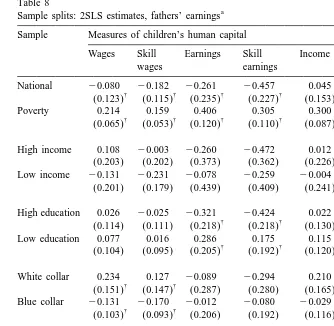
4.4. Results for low income families
My analysis to this point has implicitly assumed that the impact of parents’ income on children is the same for all families. If credit markets are imperfect, however, then income may matter more for children in poor families, since low income parents may be more likely to face binding liquidity constraints when investing in their children. Accordingly, the first two rows of Table 8 present 2SLS estimates of g splitting the full PSID sample into its representative and poverty components. The results are striking: for the poverty sample, the impact of fathers’ earnings on children’s human capital is significantly positive for each measure of human capital except for years of schooling, while for the representative sample, the impact of fathers’ earnings is negative in six of seven cases. The poverty estimates are significantly higher than the representative estimates in five of seven cases. Experiments suggested that these results are robust to using parents’ income instead of fathers’ earnings, to using each instrument separately, to allowing coefficients to differ by gender, and to using sample weights. Another interesting set of results (not in the Table) is that OLS estimates ofg are significantly lower in the poverty sample than in the representative sample when I do not control for fathers’ observable skills, but are similar when I control for fathers’ skills. Put differently, controlling for fathers’ skills has a much smaller impact on OLS
27
28
estimates in the poverty sample than in the representative sample. This suggests that fathers’ education and occupation may be less indicative of ability in the poverty sample, which is consistent with the idea that the accumulation of observable skills by poverty sample fathers may have been suboptimal due to liquidity constraints.
Why are the results for the poverty and representative samples so different? One possibility, of course, is that the true impact of income is higher among low-income families. The third and fourth rows investigate this possibility by splitting the full sample at the 25th percentile of fathers’ average annual labor income
29
($21,787 in 1988 dollars). The results do not support liquidity constraints; the 2SLS estimates of g are never significantly different across the two subsamples, and the point estimates ofg are lower in the low-income subsample in only four of seven cases.
A second possibility is that my 2SLS estimates are more upwardly biased in the poverty than in the representative sample, perhaps due to a greater correlation between union or industry and unobserved ability in the poverty sample. This conjecture is consistent with the first-stage regression results reported in Table 2; the instruments explain more variation in fathers’ earnings in the poverty sample than in the representative sample, which is what one would expect if the instruments were more endogenous in the poverty sample. On the other hand, this higher partial R-squared is due primarily to the union coefficient, which is considerably higher in the poverty sample. While it is possible that union status is more correlated with unobserved ability at low levels of income, it is also possible
28
For wages, the OLS estimate (standard error) excluding Xi21is 0.300 (0.032) in the representative sample versus 0.130 (0.023) in the poverty sample, while controlling for Xi21reduces these to 0.147 (0.044) in the representative sample versus 0.096 (0.022) in the poverty sample. For earnings, the estimates excluding X are 0.397 (0.053) in the representative sample versus 0.221 (0.047) in the poverty sample; including X reduces these to 0.197 (0.075) in the representative sample versus 0.185 (0.049) in the poverty sample. For total income, the estimates excluding X are 0.305 (0.037) in the representative sample versus 0.193 (0.032) in the poverty sample, while including X the estimates are 0.217 (0.051) in the representative sample versus 0.176 (0.033) in the poverty sample. For education, the estimates excluding X are 1.481 (0.129) in the representative sample and 0.179 (0.140) in the poverty sample, while including X the estimates are 0.507 (0.134) in the representative sample and
20.023 (0.152) in the poverty sample. When X is excluded, the representative estimate is significantly higher than the poverty estimate in all four cases; when X is included, the difference is significant only for education. The absolute value of the difference declines in all four cases.
29
Table 8
a
Sample splits: 2SLS estimates, fathers’ earnings Sample Measures of children’s human capital
Wages Skill Earnings Skill Income Skill Years
wages earnings income school
National 20.080 20.182 20.261 20.457 0.045 20.151 20.405
† † † † † †
(0.123) (0.115) (0.235) (0.227) (0.153) (0.151) (0.476) Poverty 0.214 0.159 0.406 0.305 0.300 0.199 20.083
† † † † † †
(0.065) (0.053) (0.120) (0.110) (0.087) (0.083) (0.411) High income 0.108 20.003 20.260 20.472 0.012 20.200 20.455
(0.203) (0.202) (0.373) (0.362) (0.226) (0.243) (0.837) Low income 20.131 20.231 20.078 20.259 20.004 20.185 0.867
(0.201) (0.179) (0.439) (0.409) (0.241) (0.258) (1.261) High education 0.026 20.025 20.321 20.424 0.022 20.080 20.258
† † †
(0.114) (0.111) (0.218) (0.218) (0.130) (0.138) (0.528) Low education 0.077 0.016 0.286 0.175 0.115 0.004 0.874
† † †
(0.104) (0.095) (0.205) (0.192) (0.120) (0.122) (0.400) White collar 0.234 0.127 20.089 20.294 0.210 0.005 20.075
† †
(0.151) (0.147) (0.287) (0.280) (0.165) (0.171) (0.633) Blue collar 20.131 20.170 20.012 20.080 20.029 20.098 0.341
† †
(0.103) (0.093) (0.206) (0.192) (0.116) (0.118) (0.366) White 20.004 20.089 20.046 20.205 0.103 20.056 20.096
(0.105) (0.100) (0.201) (0.194) (0.116) (0.125) (0.418) Black 20.002 20.056 0.032 20.069 0.008 20.093 0.874
(0.099) (0.102) (0.226) (0.182) (0.131) (0.139) (0.982) North 20.037 20.112 20.081 20.222 0.034 20.107 20.171
(0.126) (0.120) (0.239) (0.226) (0.142) (0.150) (0.516) South 0.035 20.042 0.077 20.066 0.058 20.084 0.022
(0.102) (0.092) (0.184) (0.174) (0.118) (0.117) (0.380)
a
This table presents estimates of the impact of fathers’ earnings the human capital accumulation of
†
children in various subsamples of the PSID. Robust standard errors are in parentheses; denotes estimates differing significantly from their opposite subsample counterpart at 5 percent.
that the true union premium is higher at low levels of income, given that unions explicitly try to compress skill differences in wages. One can therefore explain the first-stage results without asserting that the instruments are more endogenous in the low-income sample. Moreover, overidentifying restrictions tests do not suggest that instrument endogeneity is more problematic for the poverty sample than for the representative sample.
30
the full sample by fathers’ education, occupation, race and region. I find no systematic variation ing by race or region, while the only significant difference by occupation goes in the wrong direction. I do find, however, that the impact of fathers’ earnings on children’s skills is consistently higher among families whose father has less than 12 years of schooling; moreover, this difference is significant for children’s earnings, skill earnings and education. I conclude that the most likely explanation for the difference between the poverty and representative samples is that the impact of parental income on children’s skills is higher at low levels of parental education.
5. Conclusion
There can be little doubt that economic status is positively correlated across generations. However, this does not necessarily imply that parents’ income per se matters for children’s human capital accumulation. Distinguishing correlation from causality is critical to assessing the impact of policies that redistribute income among parents or invest in children’s human capital directly. In this paper, I attempt to unravel correlation and causality by isolating variation in parents’ income due to observable factors – father’s union, industry, and job loss experience – that arguably represent luck. In both the full weighted PSID sample and the nationally representative subsample, I find that changes in parents’ income due to luck have at best a negligible impact on children’s wages, earnings, years of schooling, and total family income. I find that parents’ income does have a beneficial impact on children in families whose father has less than 12 years of schooling, but not in families with low income per se. The results are generally not supportive of models in which parents’ money matters for children because of binding liquidity constraints in human capital investment.
An interesting question for future research is why parents’ income matters so little for most families. The simplest explanation is that capital markets are perfect; yet it seems unlikely that parents can actually borrow against their children’s future earnings in reality. Another explanation is that the return to human capital investment for individuals is concave, so that parents above a threshold level of
30
income would not wish to borrow against their children’s future earnings to finance additional human capital investment even if they had the opportunity; in this case, capital market imperfections not create a binding liquidity constraint. However, this explanation fails to explain why parents’ money is irrelevant in low-income families, where liquidity constraints should be most likely to bind.
Another possibility is that public investment in children is sufficiently redistri-butive to counteract inequality in parents’ resources. This story makes some sense for college, where access to financial aid (from both public and private sources) is negatively related to parental wealth (Feldstein, 1995). It makes less sense for primary and secondary education, where inequality in per-pupil spending remains large despite recent court decisions forcing some states to redistribute resources from richer to poorer districts (Murray et al., 1998). A related possibility is that school spending has no impact on educational outcomes. It is surprisingly difficult to find an empirical link between school spending and educational output, and the
31
existence of such a link remains controversial. Even if higher spending has no impact on children’s skills, however, this does not imply that parents cannot buy their children a better education. As long as schools vary in quality and school quality is known to the public, houses in good school districts will be more expensive than houses in bad districts, creating a potential link between parents’
32
income and children’s human capital.
Yet another possibility is that parents are not strictly altruistic towards their children: the fact that high-income parents should be able to send their children to better schools does not automatically mean that they will do so, even if the return
33
to additional human capital investment is high. Alternatively, parents’ income may have a negative effect on children’s own inputs of time and effort into human capital accumulation. Holtz-Eakin et al. (1993), for instance, find that recipients of large inheritances reduce their labor supply. An objection to income effects as an explanation for my results is that the children of lucky fathers do not in fact have significantly higher total income (including asset income and transfers from parents) in my sample than children of unlucky fathers. If income effects are indeed responsible for my results in the representative sample, they may take the
31
Hanushek (1986) and Heckman et al. (1996) present evidence that school spending has little effect on outcomes, while Card and Krueger (1992) and Krueger (1999) present evidence that school spending and class size matter.
32
Hanushek (1986) reports that the educational production function literature consistently finds large and persistent quality differences among schools. Black (1999), meanwhile, finds a significant positive relationship between school quality and housing prices on opposite sides of elementary school attendance boundaries in Massachusetts.
33
form of expected future inheritances, or unmeasured psychic gains from not having to work as hard in school to attain a union or high-wage industry job.
A final possibility, of course, is that my estimates are biased downwards. While I believe that my interpretation of union, industry and job status as primarily reflecting luck is defensible, I realize that some readers will disagree. I have argued that the most likely direction of bias in my 2SLS estimates under alternative interpretations of my instruments is upward, though again some may disagree. Perhaps future researchers will focus on more convincingly exogenous sources of parental income variation, such as lottery winnings or large changes in public transfers (e.g. Duflo (1999)).
Another interesting question for future research is why income is positively correlated across generations, if parents’ money has no causal impact on children’s skills. Presumably some of the correlation is due to inheritable ability, but whether this is the entire story, and whether inheritance operates primarily through genes or culture, are still open questions. It may also be the case that some other variable correlated with parental income, such as parents’ education, has a genuine causal impact on children’s skills. This is an important question, since parents’ education is potentially more responsive than genes or culture to public policy. Un-fortunately, determining the causal impact of parents’ education will be difficult, since exogenous variation in education is probably even harder to isolate than exogenous variation in income.
A final warning is that my results do not necessarily imply that public policies promoting equality of opportunity are useless or unnecessary. My data come from a specific country during a specific time period that featured large amounts of government intervention in children’s human capital accumulation. It is entirely possible that a link between parents’ income and children’s skills would emerge if this government intervention were eliminated. Future research should explore the impact of parental income using data from different time periods and different countries, in order that we might learn what sorts of public policies (if any) are the most successful at promoting social mobility.
Acknowledgements
The author thanks an anonymous referee as well as workshop participants at Wisconsin, Northwestern, NYU, Oregon, McMaster, Maryland, the Federal Reserve Board, the NBER Monetary Economics Group, Columbia, Georgetown, Johns Hopkins and the Society for Government Economists for helpful comments. The author acknowledges support from the National Science Foundation.
References