Electronic Journal of Qualitative Theory of Differential Equations 2005, No.4, 1-24;http://www.math.u-szeged.hu/ejqtde/
VISCOUS-INVISCID COUPLED PROBLEM WITH INTERFACIAL DATA
Sonia M. Ramirez
Abstract.The work presented in this article shows that the viscous/inviscid coupled prob-lem (VIC) has a unique solution when interfacial data are imposed. Domain decomposition tech-niques and non-uniform relaxation parameters were used to characterize the solution of the new system. Finally, some exact solutions for the VIC problem are provided. These type of solutions are an improvement over those found in recent literatures.
2000 Mathematics suject classification:35A07, 35A15
1. Introduction. The Navier-Stokes equation is the primary equation of computational fluid dynamics describing the flow/motion of fluids in Rn, (n = 2,3). These types of equations are often used in computations of aircraft and ship design, weather prediction, and climate modelling. By appropriate assumptions, it has been generalized to a system of equations known as the incompressible Navier-Stokes equations, see [8]. This important system has been studied for centuries by mathematicians, engineers and other scientists to explain and predict the behavior of the system under consideration, but still the understanding of the solutions to this system remains minimal. The challenge is to make substantial progress to-ward a mathematical theory which will solve the puzzle behind the Navier-Stokes equations. To make contributions to this mathematical theory, scientists have stud-ied and derived many other systems from it. Among them is the viscous/inviscid coupled problem (VIC) introduced first by Xu Chuanju in his Ph.D dissertation [15].
The work presented in this paper involves Xu’s [17] problem and focuses on three main objectives. The first one is to show the existence and uniqueness of the solution for the system, which results from the viscous/inviscid coupled problem when interfacial data (VIC-ID) are imposed. The second objective is to prove that the solution of this system can be obtained as a limit of solutions of two subproblems defined in different subdomains of the domain by using non-uniform relaxation parameters. Xu [17] used a similar techniques for the VIC problem but using lifting operators and uniform relaxation parameter. Finally, the last objective is to provide new exact solutions when all boundary conditions are satisfied in at least one of the subdomains (weaker boundary conditions) of the viscous/inviscid coupled problem, these solutions are an inprovement over those found in recent literatures. The new improvements presented in this paper demostrate progress towards the existing theory of the VIC problem and therefore for the Navier-Stokes equations.
We end this section by introducing some notation, definitions and very well known result from P.D.E that can be found [1] and [14] . Along this article we use boldface letters to denote vectors and vectors functions.
boundary ∂Ω, and let Ω− and Ω+ be two open subsets of Ω which satisfy the
following conditions
(i) Ω−∩Ω+=∅.
(ii) Ω−∪Ω+= Ω.
We define the boundaries Γ+and Γ− of the subdomains Ω+and Ω− respectively,
as follows
Γ+=∂Ω∩∂Ω+,
Γ− =∂Ω∩∂Ω−,
and the interface is given by
Γ =∂Ω−∩∂Ω+,
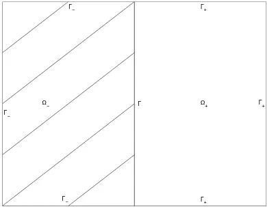
we assume Γ6=∅. Letndenote the unit normal on∂Ω to Ω, andn+,n−are the unit
normals to∂Ω+ , and∂Ω−, respectively. See figure 1 for a typical decomposition
of the domain Ω.
Ω+
Ω− Γ
Γ−
Γ−
Γ− Γ+
Γ+
Γ+
Figure 1: Decomposition of the domain Ω
We denote byL2(Ω) the space of real functions defined on Ω that are
square-integrable over Ω in the sense of Lebesgue measuredx=dx1dx2. This is a Hilbert
space with the scalar product
(u, v) =
Z
Ω
u(x)v(x)dx.
We then define the constrained spaceL20(Ω) as
L20(Ω) =
v∈L2(Ω);
Z
Ω
so L2
0(Ω) consists of all square integrable functions having zero mean over Ω. Let
D(Ω) be the linear space of functions infinitely differentiable and with compact support on Ω. Then set
D(Ω) ={φ|Ω :φ∈ D(R2)}.
For any integerm, we define the Sobolev spaceHm(Ω) to be the set of functions in
L2(Ω) whose partial derivatives of order less than or equal tombelong toL2(Ω);
i.e
The setHm(Ω) has the following properties:
(i) Hm(Ω) is a Banach space with the norm
(ii) Hm(Ω) is a Hilbert space with the scalar product
u, v
(iii) Hm(Ω) can be equipped with the seminorm
|ukm,Ω= (
Since we are dealing with 2-dimensional vector functions, we use the following notation
L2(Ω) ={L2(Ω)}2, Hm(Ω) ={Hm(Ω)}2,
and assume that these product spaces are equipped with the usual product norm (or any equivalent norm).
We defined the space H1
0(Ω) as the closure of D(Ω) for the norm k.km,Ω.
In order to study more closely the boundary values of functions of Hm(Ω), we assume that Γ, the boundary of Ω, is bounded and Lipschitz continuous, i.e. Γ can be represented parametrically by Lipschitz continuous functions. Let dσ denote the surface measure on Γ and letL2(Γ) be the space of square integrable functions
on Γ with respect todσ, equipped with the norm
kvk0,Γ={ Z
Γ
Theorem 1 (Trace Theorem). If∂Ωis bounded and Lipschitz continuous, then there exist a bounded linear mappingγ:H1(Ω)−→L2(∂Ω),such that,
(i) kγ(v)k0, ∂Ω≦ kkvk1,Ω,for all v∈H1(Ω).
(ii) γv=v|∂Ωfor all v∈ D(Ω).
Theorem 2. Withγ defined as above, we have
1. Ker(γ) =H1 0(Ω).
2. The range space ofγ is a proper and dense subspace of L2(∂Ω).
For proofs see [3] and [11]. Both theorems can be extended to vector-valued functions. functionv∈L2(Ω), we consider the pair of functionsv
−=v|Ω− andv+=v|Ω+.
We define the following inner products in Ω+ and Ω− respectively as follows:
(u+, v+)+ =
which coincides with the usual one onL2(Ω).
Consider the following space:
V={v ∈H10(Ω) :∇·v= 0}
and we denoteV⊥the orthogonal complement ofVinH1
0(Ω) for the scalar product
(∇u , ∇v) = P∂ui
∂xj∂∂xvij. Thus we have the following divergence isomorphism
Theorem 3 (Divergence Isomorphism Theorem). The divergence operator
is an isomorphism from V⊥ ontoL2
0(Ω) and satisfies
kvk1,Ω≤
1
βk∇·vk0,Ω ∀v∈ V
⊥. (1)
For a proof see Girault [7]. This theorem plays an important role in the proof of uniqueness and existence of the VIC-ID problem.
2.Viscous-Inviscid Coupled Problem with Interfacial Data.In this article we show that is it is possible to impose further conditions on the interfacial data and still have a solution to the problem. These conditions are expressed in the form of membership to certain function spaces. Specifically, we study the VIC-ID problem. Forf ∈L2(Ω), ˆg0∈H−1/2(Γ), pˆ0+∈L2(Γ), α andνpositive constants,
find two pairs (u−,u+), (p−, p+), defined in (Ω−, Ω+), satisfying the following
conditions
αu−−ν∆u−+∇p−=f− inΩ− ∇·u−= 0inΩ−
u−= 0on Γ− αu++∇p+=f+ inΩ+
∇·u+= 0inΩ+
u+n+= 0on Γ+
ν∂u−
∂n− −p−n−=p+n+ onΓ p+n+=ˆp0+ on Γ
u+n+=−u−n− onΓ
−u−n−= ˆg0onΓ;
(2)
where the domain Ω satisfies the properties mentioned previously, and the function ˆ
g0satisfies the condition
Z
Γ
ˆ
g0= 0.
In fluid mechanics this conditions is generally known as compatibility condition, see [5] and [10]. From above, the first three equations correspond to the viscous part, from fourth to sixth to the inviscid part, and the last four corresponds to the interface data. Next we prove existence and uniqueness of the solution. For that we use the saddle point theory which involves: (i) finding the weak or variational formulation of the VIC-ID problem, to describe the spaces where the interfacial data have sense. (ii) rewriting the weak formulation to find the saddle point prob-lem; which involves the definition of two bilinear formsa, band must satisfy the following conditions:
(ii) Coerciveness of the bilinear form a: a(v, v) ≧ dkvk2
X, for some positive constant d.
(iii) Continuity of the bilinear form b: | b(u, q) | ≦ ckukXkqkM, for some positive constantc.
(iv) Inf-sup condition for the bilinear form b: infq∈M supv∈X
b(v, q)
kvkXkqkM ≥β, for
some positive constantβ.
Above conditions guarantee the existence and uniqueness of the solution for the given problem, for more details see [3] and [4]. By showing the following steps we can find the weak formulation of (2).
(i) From the first and fourth equations of (2) the following inner product equa-tions are obtained
α(u−, v−)−−ν(∆u−, v−)−+ (∇p−, v−)− = (f−, v−)− (3)
α(u+, v+)++ (∇p+, v+)+= (f+, v+)+ (4)
(ii) From the second and the fifth equations of (2) we get the two pair of inner product equations
(∇·u−, q−)−= 0, (5)
and
(∇·u+, q+)+= 0; (6)
adding equations (5) and (6), we have
(∇·u+, q+)++ (∇·u−, q−)−= 0 (7)
Using the following well known identities for vector functions:
−(∆u−, v−)−= (∇u−, ∇v−)−−
Z
Γ
∂u− ∂n−v−dσ,
(∇p−, v−)−=
Z
Γ
p−v−n−dσ−
Z
Ω
∇·v−p−dx,
(∇·u+, q+)+= Z
Γ
u+n+q+dσ−(u+, ∇q+)+,
adding equations (3) and (4), and by appropriate substitutions, We have the following weak formulation of VIC-ID problem: find (u, p)∈X×M,such that for allv∈X, q∈M,
α(u, v) +ν(∇u−, ∇v−)−−(p−, ∇·v−)−+ (∇p+, v+)+= (f, v) +hˆp0+, v−iΓ
−(∇·u−, q−)−+ (u+, ∇q+)+=hgˆ0, q+iΓ
whereX,M are the two Hilbert space, defined by
X={v;v|Ω− ∈H1(Ω−), v|Ω+ ∈L
2(Ω
+),v|Γ− = 0}, (9)
M ={q;q|Ω− ∈L
2(Ω
−), q|Ω+ ∈H
1(Ω +),
Z
Ω
qdx= 0}, (10)
with respective norms
kvkX=kv−k1,Ω−+kv+k0,Ω+,
and
kqkM =kq−k0,Ω−+|q+|1,Ω+.
The VIC-ID problem is well posed in the sense that its corresponding weak formulation admits a unique solution. The statement of the theorem and proof is given below, which is one of the main results of these work.
Theorem 4. For all f ∈L2(Ω), ˆg0 ∈H−1/2(Γ), ˆp0
+ ∈L2(Γ), α and ν positive
constants, problem (8) admits a unique solution; furthermore, its unique solution
(u, p)satisfies VIC-ID problem.
Proof. The second part of the theorem is trivial. In order to prove the well posed-ness of (8), we need to apply the saddle point theory. This can be achieved by reorganizing the terms of the weak formulation by defining two bilinear formsa,b as follows:
a(u, v) =α(u, v) +ν(∇u−, ∇v−)− ∀ u∈X, ∀v∈X,
b(v, q) = (v+, ∇q+)+−(∇·v−, q−)− ∀ v∈X, ∀q∈M.
By appropriate substitutions in (8), the saddle point problem is given as: find (u, p)∈X×M such that,
a(u, v) +b(v, p) = (f, v) +hpˆ0
+, v−iΓ ∀v∈X,
b(v, q) =hgˆ0, q+iΓ ∀q∈M.
To show the above formsa, bsatisfy the conditions mentioned previously:
(i) The forma is continuous, since
|a(u,v)|≦α|(u,v)|+ν|(∇u−,∇v−)−|
≦α(|(u−,v−)−|+|(u+,v+)+|) +ν|u−|1,Ω−|v−|1,Ω− takingmax(α, ν) =cand applying Schwartz inequality,
then
| a(u, v)|≦c(ku−k1,Ω−kv−k1,Ω−+ku+k0,Ω+kv+k0,Ω+ +ku+k0,Ω+kv−k1,Ω−+ku−k1,Ω+kv+k0,Ω+). Therefore
|a(u, v)|≦ckukXkvkX.
(ii) The forma is coercive,
a(v, v) =α(v, v) +ν(∇v−, ∇v−)−
=α((v+, v+)++ (v−, v−)−) +ν(∇v−, ∇v−)−,
by definition of the inner product, we have
a(v,v) =α(|v+|20,Ω++|v−|
2
0,Ω−) +ν|v−|
2 1,Ω−, choosingmin(α, ν) =d0, and applying Schwartz inequality we get
a(v,v)≧d0(|v+|20,Ω++kv−k
2
1,Ω−)≧dkvk2X where d= d0
2.
(iii) The form bis continuous,
|b(v, q)|≦kq−k0,Ω−|v−|1,Ω−+|q+|1,Ω+kv+k0,Ω+,
since|v−|1,Ω− ≦c0 kv−k1,Ω−, and adding appropriate terms to complete the norms for the above form, we obtain
|b(v, q)|≦c0 kq−k0,Ω−kv−k1,Ω−+|q+|1,Ω+kv+k0,Ω++kq−k0,Ω−kv+k0,Ω+ + |q+|1,Ω+kv−k1,Ω−,
choosingc=max(1, c0) , it follows that
|b(v, q)|≦ckvkXkqkM.
(iv) The formbsatisfies theinf-supcondition in the spaceX×M: The objective is to decompose the general vector v into v+ and v− in such a way that inf-supcondition is satisfied.
Letq∈M, andq− can be decomposed as
q−=q−0 +r−, (11)
whereq0−∈L20(Ω−) andr−is a constant. The decomposition ofq−is justified
by the following calculation
Z
Ω−
then Z
Ω−
(q−− k1
|Ω−|)dx= 0,
where k1 is a constant,and set
q0−=q−−r−, andr−= k1
|Ω−|.
Using theorem 3 it follows that there exists a positive constant β− and a function v0
−∈H10(Ω−) such that
∇·v−0 =−q0− and kv−0k1,Ω− ≦ 1
β−kq
0
−k0,Ω−. (12)
Choosing a functiong∈X such that
Z
Γ
gn−dσ=|Ω−|,
where |Ω−| is the measure of Ω−. Let w be a function in H10(Ω−) which
satisfies:
(∇·w, q)−= (∇·g, q)− ∀q∈L2o(Ω−). (13)
To establish the existence of w we apply a special case of the saddle point theory when only one bilinear form is given. Consider the following bilinear form
ˆ b:H1
0(Ω−)×L2o(Ω−)−→R,defined as
ˆ
b(v, q) =−(v, ∇q)− ∀(v, q)∈H10(Ω−)×L2o(Ω−),
that satisfies
ˆ
b(w, q) = (∇·g, q)− ∀q∈ L2o(Ω−).
The norms for this spaces are k . kH1
0 =k . k0,Ω− andk . kL
2
o =| . |1,Ω−, respectively. Since the continuity of ˆb is obvious from the definition itself. Next step is to show that the form ˆbsatisfies theinf-supcondition as follows: takingv=−∇q, and substituting in the form ˆbwe have the following
ˆ
b(v, q) = (∇q, ∇q) =k ∇qk2
0,Ω−=k ∇qk0,Ω−|q|1,Ω− =kvk0,Ω−|q|1,Ω−.
Therefore ˆbsatisfies theinf-supcondition forβ= 1. To guarantee surjectivity of ˆbit is necessary to show that for every q ∈ L2
o(Ω−) there exists v ∈
H1
0(Ω−) such that ˆb(v, q)6= 0. By choosing v=−∇q such a way so that
it satisfies the required condition, otherwisek ∇q k2
only if qis zero. Therefore, the existence ofwis proved.
Since we prove the existences of w, then the following statement is true
(∇·w, q)−= (∇·g, q)− ∀q∈L2o(Ω−).
Letˆv−=g−w which satisfies
(∇·ˆv−, q)−= 0 ∀q∈L2o(Ω−) and
Z
Γ
ˆ
v−n−dσ=|Ω−|. (14)
By setting v−=v0−−r−vˆ−,and using relationships (11) , (12), and (14)
it follows that
v−∈H1(Ω−), v−|Γ− = 0, and
−(q−, ∇·v−)− =−(q0−+r−,∇·(v0−−r−ˆv−))−
by linearity of the inner product, we have
−(q−, ∇·v−)− =−(q−0, ∇·v0−)−+ (q−0, r−∇·vˆ−)−−(r−, ∇·v0−)−
+r−(r−, ∇·vˆ−)−.
Using the properties ofq−0,∇ˆv− and divergence theorem, it follows
−(q−, ∇·v−)− = (q0−, q−0)−+r2−
Z
Γ
ˆ
v−n−dσ,
which can be equivalently expressed in the following form
−(q−, ∇·v−)−=kq−0k20,Ω−+r
2
−|Ω−|. (15)
By applying the same procedure as in equation (11) to decomposeq+in the
subdomain Ω+ as
q+=q0++r+,
where q0
+∈H1(Ω+)∩L20(Ω−) andr+ is a constant.
Letv0
+=∇q+0,
then
(∇q+, v0+)+
kv0 +k0,Ω+
=k∇q0+k0,Ω+=k∇q+k0,Ω+=|q+|1,Ω+.
Using the fact that∇q+∈L2(Ω+), we can choosev+=v+0,
so
(∇q+, v+)+=|q+|21,Ω+, (16)
and the vectorvis characterized as follows:
v(x) =
v−(x) if x∈Ω−
Therefore,v∈X and from equations (15), and (16), we can write
and applying the linearity of the inner product in the above equation, we obtain
kq−k2
0,Ω− = (q
0
−, q−0)−+ 2(q0−, r−)−+r2−|Ω−|. (17)
By using (17) in the bilinear formb, we have
b(v, q) =kq−k2
0,Ω−−r−2|Ω−|+r−2|Ω−|+|q+|21,Ω+.
Therefore, the bilinear formbsatisfies
b(v, q)≥ kqk2M. (18) The next step is to show that the components of the vector vare bounded. Using the definition ofv− and the relationships obtained in (12), (13), and
(14), we have the following estimates
kv−k0,Ω− =kv By combining (19), (20), (21), and (22), it follows that v− satisfies the
following inequality:
kv−k1,Ω− ≤
c2
β−kq−k0,Ω−, (23)
wherec2=1+ˆβcc1
− . Using the definition ofv+ we get the following estimates:
kv+k1,Ω+≤ k∇q
0
+k0,Ω+≤ k∇q+k0,Ω+≤ |q+|1,Ω+≤ kqkM. (24)
By making use of (23) and (24), it follows that
kvkX≤
c2
sincekq−k0,Ω−≤ kqkM, we have
kvkX ≤
c2+β−
β− kqkM. (25)
Using (18) and (25), we obtain
b(v, q)
kvkX
≥ kqk
2
M c1+β−
β−
kqkM
,
and settingβ = β−
c1+β−, in the above inequality we get b(v, q)
kvkXkqkM
≥β. (26)
By taking inf-supof (26), we get the following inequality
inf q∈M vsup∈X
b(v, q)
kvkXkqkM
≥β,
which completes the proof.
3.The iteration-by-subdomain procedure and its convergence. The pur-pose of this section is to prove that the solution of VIC-ID problem can be obtained as a limit of solutions of two subproblems in the subdomains Ω− and Ω+,
respec-tively, of Ω.
Let{p˜m+}be a sequence of functions inL2(Γ) such that ˜pm+ −→p+, for some
p+∈L2(Γ).We define the sequence of function pairs (u−m, pm−)m≥1by solving for
each m the following viscous interfacial data problem in Ω−:
αum−−ν∆um−+∇pm− =f− inΩ− ∇·um
− = 0inΩ−
um− = 0inΓ−
ν∂u
m
− ∂n− −p
m
−n−= ˜pm+n+ onΓ.
(27)
We have to find the variational problem corresponding to the viscous interfacial data problem using the saddle point theory. For that we consider the first and the second equation of (27) to get the pair of inner product equations as follows:
α(um−, v−)−−ν(∆um−, v−)−+ (∇pm−, v−)− = (f−, v−)−,
(∇·um−, q−) = 0.
Using the well known identities for vector functions,
(∆um−, v−)−= (∇um−, ∇v−)−−
Z
Γ
∂u− ∂n−v−dσ,
(∇pm−, v−)− =−
Z
Γ
pm−v−n−dσ−
Z
Ω
∇·v−pm−dx,
by combining the equations in (28), and making the appropriate substitutions we can state the following weak formulation of the viscous interfacial data problem: find (um
−, pm−)∈X−×M− such that
A−[(um−, pm−), (v−, q−)] = (f−, v−)−+hp˜m+n+, v−iΓ∀(v−, q−)∈X−×M−,
(29) where
X−={v−∈H1(Ω−),v−|Γ−= 0} and M−=L(Ω−), andA− is defined by
A−[(um−, pm−), (v−, q−)] =α(um−, v−)−+ν(∇um−, ∇v−)−
−(∇·v−, pm−)−+ (∇·um−, q−)−.
The next step is to make use of the following theorem, from the Navier-Stokes equations literature( for more details see [2]) that guarantees the existence and uniqueness of the solution for the weak formulation of the viscous interfacial data problem.
Theorem 5. For allf−∈L2(Ω−)andp˜m+ ∈L2(Γ),the variational problem (29)
admits one solution; furthermore, its solution(um
−, pm−)satisfies
kum−k1,Ω−+kp m
−k0,Ω−≤c3(kfk0,Ω−+kp˜ m
+k0,Γ), (30)
wherec3 depends onαandν.
By the theorem we can define a sequence of function pairs (um
−, pm−) to state
the inviscid interfacial data problem in Ω+ as follows:
αum+ +∇pm+ =f+ inΩ+
∇·um+ = 0inΩ+
um+n+= 0inΓ+
um+n+=ϕmonΓ.
(31)
The functionsϕmare defined by:
ϕm=e−tmu−n−|
where the termse−tm , t
m are the non-uniform relaxation parameters, and these functions satisfy the following compatibility condition
Z
Γ
ϕmdσ= 0∀m.
Where{tm}is a sequence of non-negative numbers such thattm−→0 asm−→ ∞. As discussed in the viscous case, we need to find the corresponding variational problem for the inviscid interfacial data problem. From the first and the third equations of (31) we obtain the following pair of inner product equations
α(um+, v+)+(∇pm−, v+)+= (f+, v−)+,
(um+n+, q+)+=hϕm, q+i+,
(32)
and using the identity
(∇q+, um+)+= Z
Γ
q+um+n−dσ− Z
Ω
∇·um+q+dx,
the variational problem for the inviscid interfacial data problem can be stated as: find a pair of functions (um
+, pm+)∈X+×M+ such that
A+[(um+, pm+), (v+, q+)] = (f+, v+)+− hϕm, q+iΓ ∀(v+, q+)∈X+×M+,
(33) where h. , .iΓ denotes the pairing between the spaceH1/2(Γ) and its dual space
H−1/2(Γ). The formA+ is defined by
A+[(um+, pm+), (v+, q+)] =α(um+, v+)++ (v+, ∇pm+)+−(um+, ∇q+)+,
where the spacesX+ andM+ are given as:
X+=L2(Ω+),
M+=H1(Ω+)∩L20(Ω+),
and these are equipped by the following norms:
k .kX+ =k .k0,Ω+, k.kM+ =|. |1,Ω+.
The following theorem states the existence and uniqueness of the weak formulation for the inviscid interfacial data problem.
Theorem 6. For all f+ ∈ L2(Ω+)andϕm ∈ H−1/2(Γ), the variational problem
(33) admits a unique solution; furthermore, its solution (um
+, pm+) satisfies the
following condition
kum+k0,Ω++|p
m
+|1,Ω+ ≤(
1
α+ 2)kf+k0,Ω++ 2(1 +α)kϕ
mk−
If f+= 0 then the following inequalities hold
kum+k0,Ω+≤2kϕ
mk
−1/2,Γ, (35)
|pm
+|1,Ω+≤αku
m
+k0,Ω+≤2αkϕ
mk
−1/2,Γ. (36)
Proof. In order to prove the theorem Saddle point theory is used. The well
posed-ness of equation (33) can be shown by solving its equivalent saddle problem and is given as follows
a+(um+, v+) +b+(v+, pm+) = (f+, v+) ∀v+ ∈X+
b+(um+, q+) =hϕm, q+iΓ ∀q+∈M+.
(37)
The above bilinear formsa+ andb+ are defined by
a+(u, v) =α(u, v)+, ∀u,v∈X+
b+(u, q) = (v, ∇q)+, ∀v∈X+,∀q∈M+,
which has to satisfy the requirements discussed in the previous section, so that it guarantees the uniqueness of the solution of the weak problem and is given as
(i) The forma+ is continuous:
|a+(u, v)|=|α(u, v)+| ≤αkuk0,Ω+kvk0,Ω+≤αkukX+kvkX+.
(ii) the forma+ is coercive:
a+(u, u) =α(u, u)+=αkuk20,Ω+=αkuk
2
X+.
(iii) the formb+ is continuous:
|b+(u, q)| ≤ kvk0,Ω+k∇qk0,Ω+=kvk0,Ω+|q|1,Ω+=kvkX+kqkM+.
(iv) the formb+ satisfies theinf-supcondition:
By replacing v=∇q, in the bilinear formb+ and using the norms defined
above, we obtain
b+(u, q) = (v, ∇q)+= (∇q, ∇q)+=kqk20,Ω+=k∇qk0,Ω+|q|1,Ω+,
then
b+(u, q) =kvkX+kqkM+,
which implies that the form b+ satisfies theinf-sup condition for the case
Therefore, by the saddle point theory, the problem (33) has a unique solution (um
+, pm+). So the next objective is to prove the inequalities described in (34),
(35), and (36). For every pair of functionalsf+, ϕm∈L2(Ω+)×H−1/2(Γ), there
exist exactly one pair of solution (um+, pm+) corresponding to the saddle point
problem which satisfies the following conditions:
kum
In the above inequalities,β the constant of inf-supcondition ofb+ is 1, αandc
are the constants for coerciveness and continuity ofa+.
LetVandV(ϕm) be linear subspaces defined as follows:
V(ϕm) ={v ∈X+:b+(v, q) =hϕm, qi, ∀q ∈ M+}
V={v ∈X+:b+(v, q) = 0, ∀q ∈ M+};
V is a closed subspace of X+, since b+ is continuous. By the inf-sup condition
there exists um
0 ∈ V⊥ with Bum0 = ϕm, where B : X+ −→ H−1/2(Γ) is a
mapping associated tob+,defined by
hBum, q+i=b+(um, q+), ∀ q ∈ M+,
Sincea+ is coercive, the real valued function
1
2 a+(v+, v+)−(f+, v+) +a+(u m
0 , v+)
attains a minimum for somew∈V having the following property
kwkX+≤α −1(kf
+k0,Ω++cku
m
+k0,Ω+). (40)
In particular , the characterization theorem [3] implies
a+(w, v+) = (f+, v+)−a+(um0 , v+) ∀q+∈M+. (41)
The equation (39) will be satisfied if we can findpm
+ ∈M+ such that
holds. The right-hand side of (42) defines a functional in the dual spaceX′
+, since
b+satisfies theinf-supcondition, it follows that the functional can be represented
asB′pm
+ withpm+ ∈M+, which satisfies the following condition
kpm
where β and c are the constants for the inf-sup and continuity conditions for the bilinear form b+. This establishes the solvability for equation (42). Since
w = um By using inequality (40), we have
kum+kX+≤α
By combining the above terms, we obtain the following inequality
kum+kX+≤α
condition fora+, we have the following inequality
kum
From inequalities (43) and (44), we get
kpm
again by substitutingβ= 1 andc= 1 the continuity condition forb+, we obtain
kpm+kM+≤2kf+k0,Ω++ 2αkϕ
mk−
1/2,Γ. (45)
3.1 Convergence of the iteration-by-subdomain procedure.To prove con-vergence we use the fact that the relaxation parameter inϕmis non-uniform and the properties of the norms imposed on the interface Γ and the spaces X+ and
X−. The next step is to prove the sequence{ϕm}converges tou−n− with respect to the dual norm ofH12(Γ) . For that we have the following estimates:
kϕm−u−n−k
Using Schwartz inequality, we have the following
|hϕm−u−n−, µi
By using the following estimate (see [1] and [11] for further details),
kum and equation (30) in theorem 5, , we obtain the following
kum−n−k−1/2,Γ≤c4(kum−k0,Ω−+k∇.u
objective is to prove thatum
+ −u+−→0 in Ω+. By takingf+= 0, and using the
variational formA+ as discussed in section 4.1 for the inviscid problem, we have
A+[(um+ −u+, pm+−p+),(v+, q+)] =hu−n−−ϕm, q+iΓ,
and (34) from theorem 6, we get
kum+−u+k0,Ω++kp
m
+−p+kM+ ≤2(1 +α)ku−n−−ϕ
mk
Since ϕm−u−n− −→ 0 as m −→ ∞, it follows that um
+ −→ u+ in X+, and
pm
+ −→ p+inM+asm −→ ∞. By similar argument we show thatum−−u−−→
0 in Ω−. By takingf−= 0, and using the factpm−−p−∈L2(Γ),the formA−take
the form
A−[(um− −u−, pm− −p−),(v−, q−)] =h(pm− −p−)n+, v−)iΓ,
and by (30) in theorem 5, we get
kum
−−u−k1,Ω−+kp
m
− −p−k0,Ω− ≤ c3 kp˜
m
+−p+k0,Γ.
Using the hypothesis ˜pm+ −→ p+
textas m −→ ∞, it follows that um
− −→ u− inX− and pm− −→ p− as m −→
∞inM−,which concludes the proof of convergence of the iteration-by-subdomain procedure.
4. Exact solutions with weaker boundary conditions. During the investi-gation of the viscous/inviscid coupled problem we found few exact solutions with weak boundary conditions. For computational purposes it is always advantageous to have as many test functions as possible, and the visualization for analyzing and characterizing the behavior of the problem under investigation, see [12]. Also with the purpose of designing newer algorithms and testing the ones suggested by others. We briefly describe two kinds of solutions with weak boundary conditions found in earlier literatures. The first kind of solutions (u, p) are those that do not satisfy some of the boundary conditions in both subdomains, but satisfy the interface con-ditions. In such solutions the vector field component,u(x, y) = (u1(x, y),u2(x, y)),
has a particular form, in such a way that one of the component, eitheru1(x, y) = 0
oru2(x, y) = 0. In other words, the graph of the vector fielduis embedded inR3.
Almost all the solutions found in earlier articles are of this kind, see [18]). The second kind of solutions (u, p) are those that do not satisfy any of the boundary conditions but satisfy the interface conditions. In this case the graph of the vector field component is in R4. In fact only one of this kind of solution was found by Xu in his articles [16]. New examples of these solutions are found in Ramirez’s dissertation [13].
Exact solutions with weaker boundary conditions are those that satisfy all the boundary conditions in at least one of the subdomains, and the interface condi-tions. In fact these solutions are an improvement over the exact solutions with weak boundary conditions found in earlier literatures. Here we present two types of solutions, which are exponential and polynomial in nature.
Given the domain Ω as follows:
Ω ={(x, y)∈R2:−2 ≤ x ≤2 & −1≤ y ≤1},
which is decomposed into the two subdomains Ω+ and Ω− as
and
Ω−={(x, y)∈R2:−2 ≤ x ≤0 & −1≤ y ≤1}
Example 1: Exact solution with weaker boundary condition in Ω+.
Consider the following data:
(i) the external force in the subdomain Ω− is of the following form
f−(x, y) =(α[4ye1−y 2
(e1−y2−1)(e8+x3−1)2]−4νye1−y2(e1−y2−1)18x4e2(x3+8) −4νye1−y2(e1−y2−1)[6xe8+x3(e8+x3−1)(2 + 3x3)]
−ν(e8+x3−1)2[−16ye2(1−y2)[3−4y2]−ν(8e8+x3−1)2ye1−y2[3−2y2]] +πcos(πx) cos(πy), α[6x2(e1−y2−1)2e8+x3(e8+x3−1)]
−ν(e1−y2−1)2[3x2(e2(8+x3))[12x+ 18x4]
+ (e8+x3−1)e8+x3[12 + 108x3+ 54x6] +e2(8+x3)[72x3+ 108x6]] + 6x2ex3+8(ex3+8−1)[8y2e2(1−y2)
+e1−y2(e1−y2−1)[−4 + 8y2]]−πsin(πy) sin(πx)),
and
(ii) the external force in the subdomain Ω+ is of the following form
f+(x, y) =(α[4ye1−y
2
(e1−y2−1)(e8+x3−1)2] +πcos(πx) cos(πy), α[6x2(e1−y2−1)2e8+x3(e8+x3−1)]−πsin(πy) sin(πx)).
Then the vector field componentuof the exact solution in the entire domain Ω is given by
u(x, y) = (4ye1−y2(e1−y2−1)(e8+x3−1)2 ,6x2(e1−y2−1)2e8+x3(e8+x3−1)),
and the pressure component of the solution in Ω is
p+(x, y) =p−(x, y) = sin(πx) cos(πy).
−2 −1.5 −1 −0.5 0 0.5 1 1.5 2 2.5 −1
−0.8 −0.6 −0.4 −0.2 0 0.2 0.4 0.6 0.8 1
Figure 2: Velocity vectors ofuin the domain Ω
Example 2: Exact Solution with weaker boundary condition in Ω−.
The external forces in the subdomains Ω− and Ω+ are of the forms:
f−(x, y) =(α4y(1−y2)(x3−8)2−4νy(1−y2)[30x4+ 96x]−24y(x3−8)2−3x ,
α6x2(x3−8)(1−y2)2−ν(1−y2)2[120x3+ 96] + 6x2(x3−8)(−4 + 12y2) + 2y),
and
f+(x, y) = (α4y(1−y2)(x3−8)2+ 2x−2νy , α6x2(x3−8)(1−y2)2+ 2y−2νx).
Then the vector field componentuof the exact solution in the domain Ω can be written as
u(x, y) = (4y(1−y2)(x3−8)2 ,6x2(x3−8)(1−y2)2).
For the completeness of the entire solution in the domain Ω, the pressures in both subdomain Ω+ and Ω− are given as follows:
pressurep+ in the subdomain Ω+ is
p+(x, y) =x2+y2−yx ,
and pressurep− in the subdomain Ω− is
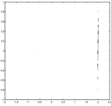
p−(x, y) =−3 2 x
Figure 3 below shows the behavior of the velocity vectors close to the bound-ary∂Ω and on the interface Γ. From the graph we can observe the smooth behavior of the velocity vectors in the inviscid part without any hindrance.
−2.5 −2 −1.5 −1 −0.5 0 0.5 1 1.5 2
−1 −0.8 −0.6 −0.4 −0.2 0 0.2 0.4 0.6 0.8 1
Figure 3: Velocity vectors ofuin the domain Ω
For more information of these solutions see [13].
5. Conclusions. We have presented in this article (i) existence and uniqueness of the viscous-inviscid coupled problem with interfacial data, when suitable con-ditions are imposed on the interface (see theorem 4). (ii) convergence of the algorithm-subdomain procedure without using lifting operators (see section 3.2). (iii) exact solutions with weaker boundary condition in at least one of the sub-domains for the viscous-inviscid coupled problem (see section 4), an improvement over those exact solutions with weak boundary conditions found in earlier litera-tures.
Acknowledments.All the reseach presented in this article was performed while the author was a Ph.D. student at Central Michigan University. I wish to thank my advisor professor Leela Rakesh for her physical interpretations of mathematical problems, which played an important role in the development of my dissertation.
References
[1] Adams, R.,Sobolev Spaces,Academic Press: New York, 1975.
[2] Begue, C. Conca, C. Murat, F. and Pironneau, O.Les `equations de Stokes at de Navier-Stokes avec des conditions aux limites sur la pression.Coll´ege de France Seminar IX, 1988.
[3] Braess, D.,Finite Elements,University Press: Cambridge, 2001 .
[4] Brezzi, F., On the Existence, Uniqueness and Approximation of Saddle Point Problems arising from Lagrange Multipliers,Anal of Numerical Analysis, 8, (1967), 129-151.
[5] Chorin, A. J., and Marsden, J. E., A Mathematical Introduction to Fluid
Mechanics,Spring-Verlag: New York, 1979.
[6] Constantin, P., Some Problems and research dDirections in the
Mathemati-cal Study of Fluid Dynamics, In Mathematics Unlimited-2001 and Beyond,
Springer Verlag.
[7] Girault, V., and Raviart P. A.,Finite Element Approximation of the Navier
Stokes Equations,Spring-Verlag: New York, 1979.
[8] Ladyzbenskaya, O. A.,The Mathematical Theory of Viscous Incompressible
flow,Gorden of Beach Science Publischer, 1969.
[9] Ladyzhenskaya, O. A., Mathematical problems of the Dynamics of Viscous
Incompressible Fluids, 2nd edition, Nauka, Moscow 1970.
[10] Landau, D., and Lifschitz, M.,Fluid Mechanics, Pergamon, 1987.
[11] Lions, J. L., Probl´emes aux Limites dans les Equations aux D´eriv´ees Par-tielles,Presses de l’Universit´e: Montreal, 1965.
[12] Marini, L., and Quarteroni, A., A Relaxation Procedure for Domain Decom-position Methods Using Finite Elements,Numerical Analysis of mathematics
55, (1989), 575-598.
[14] Temam, R.,Navier-Stokes Equations,American Mathematical Society, Rhode Island, 2001.
[15] Xu, C.,Couplage des ´equations de Navier-Stokes et d’Euler, Ph.D thesis Uni-versit´e de Pierre et Marie Curie, Paris, 1993.
[16] Xu, C., and Maday, Y., A Global Algorithm in the Numerical Resolution of the Viscous/inviscid Coupled Problem,Chinese Analysis Of Mathematics
18B (2), (1997), 191-200.
[17] Xu, C., An Efficient Method for the Navier-Stokes/Euler Coupled Equations Via Collocation Approximation,Siam Journal Of Numerical Analysis38 (4), (2000), 1217-1242.
[18] Xu, C., and Yumin, L., Analysis of the Iterative Methods for the Vis-cous/inviscid Coupled Problem Via a Spectral element Approximation,
Inter-national Journal For Numerical Methods In Fluids 32 (6), (2000), 619-646.
Sonia Ramirez
Department of Mathematics R. Daley College
7500 S. Pulaski, Chicago, IL 60652 E-mail address: [email protected]