El e c t ro n ic
Jo ur
n a l o
f P
r o
b a b il i t y
Vol. 16 (2011), Paper no. 33, pages 981–1000. Journal URL
http://www.math.washington.edu/~ejpecp/
Interpolation percolation
Martin P. W. Zerner
∗Abstract LetX ⊂Rbe countably infinite and let(Y
x)x∈X be an independent family of stationary random
setsYx ⊆R, e.g. homogeneous Poisson point processesYx onR. We give criteria for the a.s. existence of various “regular” functions f :R→ R with the property that f(x)∈ Yx for all x∈ X. Several open questions are posed.
Key words:Interpolation, path connected, percolation, stationary random set. AMS 2000 Subject Classification:Primary 60D05, 60K35; Secondary: 54D05. Submitted to EJP on July 29, 2010, final version accepted March 30, 2011.
1Address: Eberhard Karls Universität Tübingen, Mathematisches Institut, Auf der Morgenstelle 10, 72076 Tübingen, Germany.
Email:[email protected]
URL:http://www.mathematik.uni-tuebingen.de/~zerner
1
Introduction
In classical discrete percolation[Gr99]one randomly and independently deletes edges or vertices from a graph and considers the properties of the connected components of the remaining graphV. In standard continuum percolation[MR96], which is concerned with Boolean models, one removes balls, whose centers form a random point process, from space and again investigates the connectivity properties of the remaining part V of space or, somewhat more commonly, of its complementVc. In both cases, each component deleted from the underlying medium has, in some sense, a strictly positive volume. Moreover, any bounded region of the space intersects a.s. only a finite number of these components (see e.g.[MR96, Proposition 7.4]for continuum percolation).
In contrast, in fractal percolation[Gr99, Chapter 13.4]and continuum fractal percolation [Zä84] [MR96, Chapter 8.1]one may delete from any bounded open region countably many components, each of which has a strictly positive volume. For example,[Zä84]deals with the Hausdorff dimen-sion of the set V = Rn\Si∈NΓi, where Γ1,Γ2, . . . are independent random open sets inRn, the
so-called cutouts, e.g. scaled Boolean models.
In the present paper we introduce another continuum percolation model, inR2, in which countably
many components may be removed from any bounded region. However, in contrast to the previous models, these components are null sets in R2. In particular, the remaining set V ⊂ R2 has full
Lebesgue measure. The cutouts are arranged in such a way thatV exhibits various phase transitions. The precise model is the following.
Fix a complete probability space(Ω,F,P) and a countably infinite setX ⊂R. For all x ∈ X let Yx ⊆Rbe a random closed set, i.e.Yx is a random variable on(Ω,F,P)with values in the space of closed subsets ofRequipped with the Borelσ-algebra generated by the so-called Fell topology,
see[Mo05, Chapter 1.1.1]for details. Throughout we suppose that
P[Yx =;] =0 for allx ∈ X. (1)
Another common assumption will be that
(IND) (Yx)x∈X is independent,
which is defined as usual, see[Mo05, Definition 1.1.18]. We will also need to assume some transla-tion invariance of the setsYx as described in[Mo05, Chapter 1.4.1]. One such possible assumption is that
(STAT) Yx is stationary for all x ∈ X, i.e.Yx has for alla∈Rthe same distribution asYx +a.
This assumption is stronger than the hypothesis that
(1STAT) Yx is first-order stationary for all x ∈ X, i.e. for alla,b,c∈R, witha≤ b, P
Yx∩[a+c,b+c]6=; =P
Yx∩[a,b]6=;
.
Our main example, which satisfies all of the above conditions, is the following:
For a renewal process with interarrival times which are not exponentially distributed, like under (PPP), but Weibull distributed, see Example 4. Another example, which fulfills (IND) and (STAT) and is periodic, is
Yx =λx(Kx +Z+Ux), whereλx 6=0 and allKx ⊂R(x∈ X)
are compact and(Ux)x∈X is i.i.d. withUx ∼Unif[0, 1].
(2)
We now remove for eachx ∈ X the set{x} × Yc
x fromR2, whereYxc=R\Yx, and investigate the
remaining set
V :=R2\ [ x∈X
{x} × Yxc=¦(x,y)∈R2|x∈ X ⇒ y ∈ Yx©.
We thus “perforate"R2by cutting out random subsets of parallel vertical lines to obtain a “vertically
dependent" random setV ⊂R2. For a similar discrete percolation model with vertical dependence
see[Gr09, Section 1.6].
What are the topological properties ofV? It is easy to see thatV is always connected, see Proposition 5. However, whetherV is path-connected or not depends on the parameters. (Recall thatV is path-connected if and only if for allu,v∈V there is a continuous function f :[0, 1]→V with f(0) =u
and f(1) =v.)
Theorem 1. Assume (PPP) and letX be bounded. Then V is a.s. path-connected if
∀ǫ >0 X
x∈X
e−λxǫ<∞, (3)
and a.s. not path-connected otherwise.
Example 1. Assume (PPP), supposeX is bounded and let (xn)n∈Nenumerate X. ThenV is a.s.
path-connected if logn=o(λxn)and a.s. not path-connected ifλxn=O(logn), cf. Example 3.
Note that (3) depends only on the intensitiesλx, counted with multiplicities, but not onX itself.
Theorem 1 will be generalized in Theorem 4. There it will also be shown that V is a.s. path-connected if and only if there is a continuous function f : R → R whose graph graph(f) := {(x,f(x)) | x ∈R} is contained in V. This brings up the question under which conditions there are functions f :R→Rwhich have other regularity properties than continuity and which belong
to
I :=
f :R→R|graph(f)⊆V =
f :R→R| ∀x ∈ X : f(x)∈ Yx .
0.2 0.4 0.6 0.8 1.0
-0.3 -0.2 -0.1 0.0 0.1 0.2
Figure 1: (a) In the left figurexn,n∈N, are independent and uniformly distributed on[0,1],X={xn: n∈N}, and Yxn,n∈N, are independent Poisson point processes of intensityλxn=n, independent also of(xn)n∈N. The figure shows
Yx1, . . . ,Yx20and an interpolating continuous functionf ∈ Iwith f(0) =f(1) =0. (b) In the right figureX ={2, 3, . . .}
andYn= [1/n, 1] +Z+Un, whereUn,n≥2, are independent and uniformly distributed on[0,1]. The figure shows Y2, . . . ,Y11and an interpolating line, see also Open Problem 3.
functions with various regularity properties, occur or don’t occur.
B :=
∃f ∈ I : f is bounded (see Prop. 3),
C :=
∃f ∈ I : f is continuous (see Th. 4),
M := ¦∃f ∈ I : f is increasing1and bounded© (see Th. 6),
BV :=
∃f ∈ I : f is of bounded variation (see Th. 7),
LK :=
∃f ∈ I : f is Lipschitz continuous with Lipschitz constantK , whereK>0, (see Th. 10),
Pm :=
∃f ∈ I : f is a polynomial of degreem ,
wherem∈N0={0, 1, 2, . . .}, (see Prop. 11, Th. 12),
A :=
∃f ∈ I : f is real analytic (see Prop. 13).
It will follow from the completeness of(Ω,F,P)that these sets are events, i.e. elements ofF. Our results forB,PmandAare not difficult.
Remark 1. (0-1-law)Note that every event defined above, call itG, is invariant under vertical shifts ofV, i.e.Goccurs if and only if it occurs after replacingV by anyV+(0,a),a∈R. Therefore, under
suitable ergodicity assumptions, P[G]∈ {0, 1}. This is the case if (PPP) holds. In general, e.g. in case (2), this need not be true, see Remark 10.
Remark 2. (Monotonicity)There is an obvious monotonicity property: IfX is replaced byX′⊆ X
and(Yx)x∈X by(Yx′′)x′∈X′ withY′
x′⊇ Yx′ for allx′∈ X′thenV andI and all the events defined
above and their probabilities increase.
Remark 3. (Closedness)There are various notions of random sets. Random closed sets seem to be
the best studied ones, see[Mo05]and Chapter 1.2.5 therein for a discussion of non-closed random sets. For this reason we assume the sets Yx to be closed even though this assumption does not
1Here and in the following a function
seem to be essential for our results. An alternative, but seemingly less common notion of stationary random and not necessarily closed sets is described e.g. in[JKO94, Chapter 8].
Remark 4. (Further connections to other models)This model is related to various other models
in probability.
(a) (Brownian motion) Our construction of the continuous functions in the proof of Theorem 1 has been inspired by Paul Lévy’s method of constructing Brownian motion. In Example 4 we shall even choose X ⊆ (0, 1] and (Yx)x∈X in a non-trivial way and use this method to define a Brownian motion(Bx)0≤x≤1 on the same probability space(Ω,F,P)such that a.s.(Bx)x∈R∈ I. (Here we let Bx :=0 for x∈/(0, 1]to extendB·(ω)to a function defined onR.)
(b) (Lipschitz and directed percolation) In[DDGHS10]random Lipschitz functionsF :Zd−1 →Z
are constructed such that, for everyx∈Zd−1, the site(x,F(x))is open in a site percolation process
onZd. The cased=2 is easy since it is closely related to oriented site percolation onZ2. However,
if we let d=2, denote the Lipschitz constant by L and let the parameterpL of the site percolation process depend onLsuch thatL pL→λ∈(0,∞)asL→ ∞then we obtain after applying the scaling
(x,y)7→(x,y/L)in the limit L → ∞the problem of studying the event L1 under the assumption
(PPP) withX =Zandλx =λfor all x ∈ X. Theorem 10 deals with this case and is proved using oriented percolation.
(c) (First-passage percolation) Our computation ofP[BV]in Theorem 7 applies a method used for the study of first-passage percolation on spherically symmetric trees in[PP94].
(d) (Intersections of stationary random sets) Note that
P0=
n \
x∈X
Yx 6=;o. (4)
Such intersections of stationary random sets (or the unions of their complements) have been inves-tigated e.g. in[Sh72a], [Sh72b], [KP91]and[JS08]. Studying the events Pm ⊇ P0, m≥1, yields
natural variations of these problems, see e.g. Open Problem 3.
(e) (Poisson matching) In 2-color Poisson matching[HPPS09]one is concerned with matching the points of one Poisson point process to the points of another such process in a translation-invariant way. In our model with assumption (PPP),∞-color Poisson matching would correspond to choosing infinitely many f ∈ I in a translation-invariant way. This will be made more precise in Open Problem 6.
2
Results, proofs, and open problems
Some of our results will be phrased in terms of the following random variables. We denote for
x ∈ X andz∈Rby
D+x(z) := inf{y−z: y ≥z, y ∈ Yx},
D−x(z) := inf{z−y: y ≤z, y ∈ Yx}, and
Dx(z) := inf{|y−z|: y ∈ Yx}=min{D+x(z),D−x(z)}
Lemma 2. The probability that Dx(z)is finite for all x∈ X and all z∈Ris 1. If (1STAT) holds then the distributions of Dx(z),D+x(z)and D
−
x(z)do not depend on z and2Dx(0)has the same distribution as D+x(0)and D−x(0).
Proof. The first statement follows from{∀z∈R:Dx(z)<∞}={Yx 6=;}and (1). If (1STAT) holds
then
P[Dx(z)≤t] =P[Yx∩[z−t,z+t]6=;] =P[Yx∩[−t,t]6=;] =P[Dx(0)≤t].
Similarly,P[D+x(z)≤t] =P[D+x(0)≤t] =P[Dx(0)≤t/2]. Analogous statements hold forD−x.
Example 2. Under assumption (PPP) all three distancesD+x(z),Dx−(z)andDx(z)are exponentially distributed with respective parametersλx,λx, and 2λx.
For comparison with Theorem 4 about continuous functions and as a warm-up we first consider bounded, but not necessarily continuous functions.
Proposition 3. (Bounded functions)Assume (IND). If
sup
x∈X
Dx(0)<∞ a.s. (5)
then P[B] =1, otherwise P[B] =0.
Proof. If (5) holds then a bounded functionf ∈ I can be defined by setting f(x) =0 forx ∈ X/ and choosing f(x)∈ Yx with|f(x)|= Dx(0)for all x ∈ X. For the converse we note that any f ∈ I
must satisfykfk∞≥supx∈XDx(0)and apply Kolmogorov’s zero-one law.
Remark 5. By the Borel Cantelli lemma (5) is equivalent to
∃t <∞ X
x∈X
P[Dx(0)>t]<∞. (6)
Note that (5) and (6) do not depend onX but only on the distributions of the random variables
Dx(0), x∈ X.
Example 3. Suppose (PPP) holds and(xn)n∈NenumeratesX. ThenP[B] =1 if logn=O(λx
n)and P[B] =0 ifλxn=o(logn), cf. Example 1.
Theorem 1 immediately follows from the following result.
Theorem 4. (Continuous functions)Assume (IND) and (1STAT). If
∀m∈N ∀ǫ >0 X
x∈X,|x|≤m
P[Dx(0)> ǫ]<∞ (7)
then P[V is path-connected] =P[C] =1.Otherwise, P[V is path-connected] =P[C] =0.
Remark 6. Suppose(xn)n∈NenumeratesX. Then, by the Borel Cantelli lemma, (7) is equivalent
to
∀m∈N lim
n→∞Dxn(0)1[−m,m](xn) =0 a.s.. (8)
Compare (7) to (6) and (8) to (5). Also note that ifX is bounded then (7) does not depend onX
Proof of Theorem 4. Assume (7). Then for all y ∈ Rand all ǫ >0 the set X(y,ǫ) := {x ∈ X | Dx(y)≥ǫ/3}is a.s. locally finite due to the Borel Cantelli lemma and Lemma 2. Therefore, for all K,ǫ >0 the set
XK(ǫ):={x ∈ X | ∃y∈[−K,K]:Dx(y)≥ǫ}
is a.s. locally finite as well since it is contained in the union of the setsX(y,ǫ)with y ∈[−K,K]∩ (ǫ/3)Z. This together with (1) and the monotonicity ofXK(ǫ) inK and inǫimplies the existence
of a setΩ′⊆Ωof fullP-measure on which
∀K,ǫ >0 :XK(ǫ)is locally finite and ∀x ∈ X :Yx6=;. (9)
For the proof of the first statement of the theorem it suffices to show that on Ω′ there is for all
a0,a1,b0,b1∈Rwitha0<a1some continuous function f = fa
0,a1,b0,b1:[a0,a1]→Rwith
f(a0) =b0, f(a1) =b1 and f(x)∈ Yx for all x∈ X ∩]a0,a1[. (10)
Indeed, this immediately shows that onΩ′any two points inV with differing first coordinatesa0and
a1can be connected by a continuous path insideV. Points inV whose first coordinates coincide can
be connected by the concatenation of two such paths. Similarly,P[C] =1 follows by concatenating the functions fa
n,an+1,0,0, where(an)n∈Zis a strictly increasing double sided sequence inR\X with
an→ ∞anda−n→ −∞as n→ ∞.
Therefore, let a0,a1,b0,b1∈Rwitha0<a1. IfX ∩]a0,a1[is finite then the existence of a
contin-uous function fa0,a1,b0,b1 satisfying (10) is obvious. Now assume thatX ∩]a0,a1[is infinite. Also fix
a realization inΩ′. By (9),
K:= sup
Dx(0):x∈ X1(1)∩]a0,a1[ ∨ |b0| ∨ |b1|
+2 (11)
is finite. Here sup;:=0. The setsAn,n∈N0, recursively defined by
An:=
XK(2−n)∩]a0,a1[
\
n−1
[
k=0
Ak (n∈N0),
are finite due to (9), pairwise disjoint and satisfy
[
n≥0
An=[ n≥0
XK(2−n)∩]a0,a1[= X ∩]a0,a1[
\{x∈ X :[−K,K]⊆ Yx}. (12)
We shall obtain the desired function f = fa0,a1,b0,b1 as uniform limit of a sequence(fn)n≥0of
contin-uous functions which satisfy for alln≥0,
fn:[a0,a1]→ K−2+
n−1
X
k=0
2−k
!
[−1, 1]⊆[−K,K], (13)
fn(a0) =b0, fn(a1) =b1, (14)
fn(x)∈ Yx for allx ∈An, (15)
fn(x) = fn−1(x) for allA0∪. . .∪An−1ifn≥1, and (16)
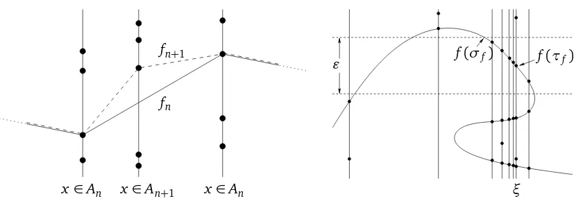
fn fn+1
x ∈An x∈An x ∈An+1
ǫ
ξ
f(τf) f(σf)
Figure 2: For the proof of Theorem 4 in case (PPP).
We construct this sequence recursively. For n=0 set f0(a0) = b0, f0(a1) = b1 and choose f0(x)∈
Yx for all x ∈ A0 such that |f0(x)| = Dx(0). This defines f0(x) for finitely many x. By linearly interpolating in between these values we get a continuous piecewise linear function f0 satisfying (13)–(17) withn=0.
Now letn≥0 and assume that we have already constructed a continuous function fn which fulfils
(13)–(17). We then set fn+1(x) = fn(x)for all x ∈ {a0,a1} ∪A0∪. . .∪An. For all x ∈An+1, which
again is a finite set, we choose fn+1(x) as some element ofYx with distance Dx(fn(x))from fn(x)
and again interpolate linearly to obtain a piecewise linear continuous functionfn+1, see Figure 2 (a).
Obviously, this function satisfies (14)–(16) withn+1 instead ofn. To see that the same is true for (13) and (17) we note that for all x ∈An+1, by (13), fn(x)∈[−K,K]. Therefore, Dx(fn(x))≤2−n since x∈ X/ K(2−n). Hence|fn+1(x)−fn(x)| ≤2−n. Consequently, since we interpolated linearly,
kfn− fn+1k∞=sup
|fn+1(x)−fn(x)|: x ∈An+1 ≤2−n, (18)
i.e. (17) holds withn+1 instead ofn. This together with (13) implies that (13) also holds forn+1 instead ofn.
Having finished the construction of(fn)n≥0, we see that it converges uniformly on[a0,a1] due to (17) to some function f. Since all the functions fn are continuous f is continuous as well. It also
fulfils (10) due to (12)–(16).
For the proof of the converse assume that there are m ∈ N and ǫ > 0 such that P
x∈X,|x|≤mP[Dx(0)> ǫ] = ∞. Since [−m,m] is compact there isξ∈[−m,m]such that for all
δ >0 the sum of the probabilitiesP[Dx(0)> ǫ]withx ∈ X ∩(ξ−δ,ξ+δ)diverges. Without loss of generality we may assume that one can chooseξ∈[−m,m]such that even
X
x∈X ∩(ξ−δ,ξ)
P[Dx(0)> ǫ] =∞ for allδ >0. (19)
(Otherwise replaceX by −X.) Denote by C2 the event that there is a continuous function f =
(f1,f2) : [0, 1]→ R2 with f1(0) < ξ < f1(1) whose graph is contained in V. Note that C ⊆ C2
and{V is path-connected} ⊆C2. Therefore, it suffices to show P[C2] =0. For any such function
f define τf :=min{t ∈[0, 1]| f1(t) = ξ}. Since f1 is continuousτf is well-defined. Next we set
σf :=sup ¦
t∈[0,τf]: |f2(t)−f2(τf)| ≥ǫ/2 ©
τf, see Figure 2 (b). Therefore, f1(σf)< ξby definition ofτf. Consequently,
C2= [ j∈Z,k∈N
∃f ∈C[0, 1],R2 : f1(0)< ξ <f1(1), graph(f)⊂V,
|f2(τf)−jǫ| ≤ǫ/2, f1(σf)< ξ−1/k .
If f1(σf)< ξ−1/k then there is by the intermediate value theorem for all x ∈ X ∩(ξ−1/k,ξ)
somet ∈(σf,τf)with f1(t) =x. For such t we have on the one hand by the definition ofσf that
|f2(t)− f2(τf)| < ǫ/2 and on the other hand f2(t)∈ Yx since graph(f) ⊂ V. Therefore, by the
triangle inequality,
C2⊆
[
j∈Z,k∈N
Cj,k, where Cj,k:=
∀x∈ X ∩(ξ−1/k,ξ): Dx(jǫ)≤ǫ ∈ F.
Consequently, it suffices to show thatP[Cj,k] =0 for all j∈Z,k∈N. However, by (IND), (1STAT)
and Lemma 2,
P[Cj,k] =
Y
x∈X ∩(ξ−1/k,ξ)
1−P[Dx(0)> ǫ] (19)
= 0.
WhetherV is path-connected or not thus depends on the parameters of the model. One may wonder whether the same is true for the connectedness ofV. This is not the case. V is always connected as the following non-probabilistic statement shows when applied toU=V andX =R\X.
Proposition 5. (Connectedness)Let U⊆R2with projectionπ[U] =Ronto the first coordinate and
let X ⊆Rbe dense inRwith X ×R⊆U. Then U is connected.
Proof. Assume thatU is not connected. Then there are non-empty open setsO1,O2 ⊆R2 such that U∩O1andU∩O2partitionU. SinceR=π[U] =π[O1]∪π[O1]is connected and the setsπ[O1]and
π[O2]are both non-empty and open, the setπ[O1]∩π[O2]is not empty either. Since it is also open andX is dense inRthere isx ∈X∩π[O1]∩π[O2]. For anyi=1, 2,Ui:= ({x}×R)∩Oi6=;because
of x ∈π[Oi]. Moreover,{x} ×R⊆U due to X×R⊆U. Therefore,U1 andU2 partition{x} ×R
and are non-empty and open in{x} ×R. This is a contradiction since{x} ×Ris connected.
Example 4. (Interpolation by Brownian motion)The construction of an interpolating continuous
function in the proof of Theorem 4, see in particular Figure 2 (a), resembles Paul Lévy’s construction of Brownian motion, see e.g.[MP10, Chapter 1.1.2].
We shall show that one can indeed chooseX ⊆(0, 1]and, in a non-trivial way, (Yx)x∈X and then construct by Lévy’s method a Brownian motion(Bx)x∈[0,1]on(Ω,F,P)such that a.s.(Bx)x∈R∈ I.
(HereBx :=0 forx ∈/[0, 1].) Like in Lévy’s construction we letX be the set of dyadic numbers in
(0, 1], namely the disjoint unionX :=X−1∪Sn≥1Xn, whereX−1:={1}andXn :=
k2−n 1≤ k<2n, kis odd forn≥1. Forn=−1, 1, 2, 3, . . . andx ∈ Xn letYx ⊂Rbe a two-sided stationary
(in the sense of (STAT), see e.g.[KT75, Theorem 9.9.1]) renewal processes with i.i.d. interarrival times whose cumulative distribution function is given by Fn(t):=1−exp
−2n−2t2fort ≥0 and whose probability density function we denote byfn. Furthermore, we assume (IND). Forx ∈ X and
Dx(z). We then recursively defineBx for x ∈ {0} ∪ X as follows: We set B0:=0 andB1 :=Y1(0). Consequently, by symmetry Yx(z)−z is normally distributed with mean 0 and variance 2−n−1 as it should for Lévy’s construction. Continuing as in the proof of[MP10, Theorem 1.3]the function
(Bx)x∈X can be a.s. extended to a standard Brownian motion(Bx)x∈[0,1].
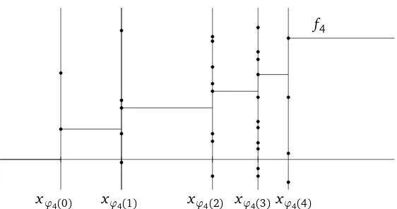
Theorem 6. (Increasing, bounded functions) Assume (IND) and (1STAT). Then P[M] = 1 if
P
satisfies the requirements formulated in the definition ofM, as we shall explain now.
xϕ4(0) xϕ4(1) xϕ4(2) xϕ4(3) xϕ4(4)
which is, by assumption, strictly less than 1 and therefore, by Kolmogorov’s zero-one law, equal to 0.
Remark 7. In Theorem 6 one can replaceD+x(0)byDx(0)due to Lemma 2.
Example 5. Assume (PPP). Then, by the three series theorem and Theorem 6,P[M] =1 if
X
one of the following conditions(22)–(24)holds:
(λn)n∈N is increasing and
Open Problem 1. (a) Theorem 7 and Example 5 do not determineP[BV]in some cases in which
(λn)n≥0 is a permutation of, say,(nlogn)n≥2. (b) Can Theorem 7 be extended toX whose closure
contains an interval?
The following non-probabilistic lemma is needed for case (24).
Lemma 8. Let(µn)n≥0 be a sequence of positive numbers which monotonically decreases to 0. Then
lim sup
Remark 8. In fact, (25) and (26) are equivalent.
Proof of Lemma 8. Letǫ:=lim supn→∞ nµn >0 and letϕ be a permutation ofN0. We inductively
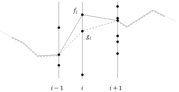
i−1 i i+1
fi
gi
Figure 4:The dashed graph has a smaller total variation than the solid graph.
For the proof of Theorem 7 we first show in Lemma 9 that whenever there is a function of bounded variation in I then there is also another such function which is only “jumping between nearest neighbors". More precisely, we recursively define the random function g:Sn∈N0{+,−}
n→Rsuch
that g(s1, . . . ,sn)∈ Yn forn≥1 by settingg(λ):=0, whereλis the empty sequence, i.e. the only
element of{+,−}0, and
g(st):=g(s) +t D|st|t (g(s)) fors∈ [
n∈N0
{+,−}n,t∈ {+,−}, (30)
wherest is the concatenation ofsandt and| · |denotes the length of a sequence. For any (finite or infinite) sequences= (si)1≤i<N+1of lengthN≤ ∞we let
gs:= (g(s1, . . . ,si))0≤i<N+1.
Moreover, for any finite of infinite sequence h= (h0,h1, . . .) of real numbers we define the total variation ofhasV(h):=Pi|hi−hi−1|.
Lemma 9. LetX =N. Then BV ⊆BV2:=
¦
∃s∈ {+,−}N
:V(gs)<∞©.
Proof. Letf ∈ I be of bounded variation. Set f0:=0 andfi:= f(i)fori∈N. We define inductively
fori∈N,
si:=sign fi−g(s1, . . . ,si−1)
∈ {+,−}, where sign 0 := +, (31)
and sets:= (si)i∈N. Thus(gi)i≥0:= gs is the sequence which starts at 0 and tries to trace (fi)i≥0
but is restricted to making only the smallest possible jumps up or down. To prove V(gs)<∞we consider for alln∈Nthe telescopic sum
V(f0, . . . ,fn)−V(g0, . . . ,gn) = V(g0,f1, . . . ,fn)−V(g0, . . . ,gn)
= n X
i=1
V(g0, . . . ,gi−1,fi, . . . ,fn)−V(g0, . . . ,gi,fi+1, . . . ,fn). (32)
(g0, . . . ,gi−1,fi, . . . ,fn)and(g0, . . . ,gi,fi+1, . . . ,fn)differ only in thei-th term the i-th summand in
if si = −. Due to the triangle inequality the expression in (33) is non-negative. Hence, by (32), V(g0, . . . ,gn)≤V(f0, . . . ,fn)and therefore
which is less than or equal to the total variation of f, which is finite.
Proof of Theorem 7. First consider case (22). By Lemma 9 is suffices to showP[BV2] =0. The proof goes along the same lines as part of the proof of[PP94, Theorem 3], which gives a criterion for explosion of first-passage percolation on spherically symmetric trees. By definition ofBV2,
P[BV2] = P
This is the sum of independent exponentially distributed random variables with respective param-eterλi, see Example 2. To apply standard large deviation estimates we weight the summands to
make them i.i.d. and consider first the sum
V∗(gs):=
ofn independent random variables which are all exponentially distributed with parameter 1. We chooseǫ >0 such that 2e2ǫ<3, denote by+n the only element of{+}n and get
which is summable inn. Therefore, by the Borel Cantelli lemma, there is a.s. some randomN such that
Mn∗:= min
s∈{+,−}nV
Recalling (35) we have for alln∈Nands∈ {+,−}n,
The second summand in (39) is equal to
ǫ
Therefore, the right hand side of (39) is equal to
ǫ
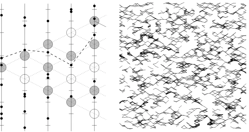
Figure 5: Here we assume (PPP) and X = Z. (a) Vertices of a quadrant of G are indicated as discs, the edges connecting them are dotted. Discs are shaded, i.e. open, if and only if there is a point of the Poisson point process in the corresponding interval. The graph of some Lipschitz function accompanying an open directed path is dashed. (b) Here λx =1 for allx∈ X. The figure shows those straight line segments whose end points(x,yx)and(x+1,yx+1)satisfy x∈ {1, 2, . . . , 50}; yx∈ Yx∩[0, 50], yx+1∈ Yx+1∩[0, 50]and|yx+1−yx| ≤K=1. Do these line segments contain the graph of a function defined on[1,50]?
In case (23) there is some finite constant c such that X′ := {x ∈ X : λx < c} is infinite. Since
X′⊆ X and(λx)x∈X′≤(c)x∈X′ the claim follows from (22) and monotonicity (Remark 2).
Case (24) is treated similarly. We choose a permutationϕ ofNsuch thatλ(n)= λϕ−1(n) for alln.
Applying Lemma 8 toµn :=1/λ(n) gives a setX′ := M ⊆ N0 such that the increasing sequence
(λ′x)x∈X′ withλ′
x :=maxn∈X′:n≤xλn≥λx satisfies P
x∈X′1/λ′x =∞. The statement now follows
from case (22) by monotonicity (Remark 2).
Theorem 10. (Lipschitz functions)Denote by pc the threshold for oriented site percolation on the
square latticeZ2. Then there is
λc∈ −[1, 3]
2 ln(1−pc), (41)
with the following property: If (PPP) holds,X =Z,K>0andλ >0is such thatλx =λfor all x ∈ X then
P[LK] =0 ifλ < λc/K and P[LK] =1 ifλ > λc/K. (42)
Proof. By independence of(Yx)x∈X and ergodicity of eachYx, P[LK]∈ {0, 1}, see Remark 1. Since P[LK]is increasing inλfor everyK, see Remark 2, there exists for allK someλc(K)∈[0,∞]with
property (42). Scaling V by (x,y) 7→(x,y/K) reduces the problem to considering Poisson point processes of intensityλK and Lipschitz functions with Lipschitz constant 1. This implies thatλc(K)
in fact does not depend onK.
(S(x,i),S(x +1,i))and(S(x,i),S(x+1,i+ (−1)x)), where x,i∈Z. This graph is isomorphic to
the oriented square lattice, see Figure 5 (a). We declare the vertexS(x,i)to be open if it intersects
{x} × Yx and to be closed otherwise. Denote byO the event that there is a double infinite directed path in G between open nearest neighbors. Any such path induces some f ∈ I with Lipschitz constant 6. Therefore,O ⊆ L6. Since any vertex is open with probability 1−e−4λ this yields the
upper bound onλc = λc(6) in (41). Conversely, any f ∈ I with Lipschitz constant 2 induces an open double infinite directed path inG. HenceL2⊆ O. This implies the lower bound onλc=λc(2)
in (41).
Remark 9. Substituting Bishir’s [Bi63] [PF05, Theorem 4.1]lower bound pc ≥2/3 and Liggett’s
[Li95]upper boundpc≤3/4 into (41) yields 0.549≤λc≤2.08. The lower bound can be improved
by directly applying the methods described in[Du84, Section 6].
Open Problem 2. What is the exact value of λc? Critical thresholds in (oriented) percolation
are rarely explicitly known. However, due to Monte-Carlo simulations, see also Figure 5 (b), we conjectureλc=1.
In the following simple example the correspondingλc can be computed explicitly.
Example 6. Let X = Z andλ,K >0. Let (Un)n∈Z be independent and uniformly distributed on
[0, 1]and set Yn := (Un+Zn)/λ forn∈Z. (Note the similarity of V to perforated toilet paper.)
Then for anyn∈Zandz∈Rthere is some y ∈ Yn with|z−y| ≤K if 2K≥1/λ. If 2K<1/λthen there is at most one such y and with positive probability no such y. HenceP[LK] =1 ifλ≥1/(2K)
andP[LK] =0 else. Thus in this case (42) holds forλc=1/2.
Next we consider some of the smoothest functions, polynomials and real analytic functions.
Proposition 11. (Polynomials)Assume (IND) and (STAT) and that allYx, x∈ X, are a.s. countable.
Then P[Pm] =0for all m∈N0.
} is a.s. countable and, by continuity, compact as well. If Pm occurs then
GK∩ Yxm+16=;for someK ∈N. By (IND) and (STAT), the closed set GK∩ Yxm+1 has for alla∈R
Of course, the assumption of countability in Proposition 11 cannot be dropped. Here is a nontrivial example. Let(xn)n∈NenumerateX and let 1> ℓ1≥ℓ2≥. . .≥ℓn→0 asn→ ∞. We consider two
different families(Yx)x∈X. The first one is of the type described in (2) and is given by
Yx
cf. Figure 1 (b). The second one consists of complements of Boolean models:
Yxn= (]0,ℓn[+Yn′)c, where(Yn′)n≥1 are independent
Poisson point processes with intensity 1. (44)
In case (43), P[0∈ I] =Qn≥1(1−ℓn), while in case (44), P[0∈ I] = Q
n≥1e−ℓn. Therefore, in
either caseP[0∈ I] =0 if and only ifPnℓn=∞. Obviously,{0∈ I } ⊆P0. However, the following
theorem due to L. A. Shepp shows that these two events might differ by more than a null set. To recognize it recall (4) and take complements.
Theorem 12. (Constant functions,[Sh72a],[Sh72b, (42)])Assume (43) or (44). Then P[P0] =0
if and only if
X
n≥1
1
n2exp n X
i=1
ℓi
!
=∞. (45)
Remark 10. Note that in case (43) there is no zero-one law like in Remark 1: 0< P[P0]< 1 is
possible. In fact,P[P0] =1 if and only ifPnℓn≤1, which is not the opposite of (45).
Open Problem 3. Let m ∈ N. Assuming (43) or (44), find conditions which are necessary and
sufficient for P[Pm] =0 (respectively,P[Pm] =1).
For m= 1 and case (43) (see also Figure 1 (b)) this problem can be phrased in terms of random coverings of a circle in the spirit of[Sh72a]and[JS08]as follows: Arcs of lengthℓx (x ∈ X) are
thrown independently and uniformly on a circle of unit length and then rotate at respective speed
x around the circle. Give a necessary and sufficient condition in terms of (ℓx)x∈X and X under
which there is a.s. no (resp., a.s. at least one) point in time at which the circle is not completely covered by the arcs. In other words: Under which conditions is there a.s. no (resp., a.s. at least one) random, but constant speed at which one can drive along a road with infinitely many independent traffic lights without ever running into a red light?
Proposition 13. (Real analytic functions)IfX is locally finite then P[A] =1.
Proof. Choose yx ∈ Yx for all x ∈ X. By [Ru87, Theorem 15.13] there is an entire function g : C→C,g(z) =P
n≥0anzn, such that g(x) = yx for allx ∈ X. Its real partℜ(g(z)) = P
n≥0ℜ(an)zn
restricted toRis real analytic and takes values yx at x∈ X as well.
We conclude by suggesting some further directions of research.
Open Problem 4. Theorem 10 and Proposition 13 deal only with locally finiteX. What can be said
about P[LK]andP[A]for more generalX? It is easy to see that even in case (PPP) with constant intensitiesλx =λany general criterion for, say,P[LK] =0 would need to depend not only onλbut
also onX itself. IfX is for example bounded then for anyK >0, P[LK]≤P[C] =0 by Theorem 4, no matter how largeλis, in contrast to (42).
Open Problem 5. One might consider other types of interpolating functions. For example, under
Open Problem 6. (More than just one function) Let X ⊂ [0, 1] and fix (λx)x∈X with λx >
0. Under which conditions is there a simple point process N =Pi∈Nδfi (in the sense of [DV88,
Definition 7.1.VII]) on the spaceC([0, 1])of continuous functions on [0, 1](or any other suitable space of regular functions) such that (a) for allx ∈ X the points fi(x), i∈N, are pairwise distinct,
(b) there are independent homogeneous Poisson point processesYx, x ∈ X, with intensitiesλx such
that{fi(x): i∈N} ⊆ Yx for allx∈ X and (c) the “vertically shifted" point processPi∈Nδfi+y has
for all y∈Rthe same distribution asN?
References
[Bi63] J. BISHIR. A lower bound for the critical probability in the one-quadrant
oriented-atom percolation process.J. R. Stat. Soc., Ser. B25, 401–404 (1963). MR0168047
[DV88] D. J. DALEY and D. VERE-JONES. An Introduction to the Theory of Point Processes.
Springer, New York (1988). MR0950166
[DDGHS10] N. DIRR, P. W. DONDL, G. R. GRIMMETT, A. E. HOLROYD, and M. SCHEUTZOW. Lipschitz
percolation.Elect. Comm. in Probab.15, 14–21 (2010). MR2581044
[Du84] R. DURRETT. Oriented percolation in two dimensions.Ann. Prob.12, no. 4, 999–1040
(1984). MR0757768
[Gr99] G. GRIMMETT.Percolation.2nd ed., Springer, Berlin (1999). MR1707339
[Gr09] G. GRIMMETT. Three problems for the clairvoyant demon.Probability and
Mathemat-ical Genetics (N. H. Bingham and C. M. Goldie, eds.), Cambridge University Press, Cambridge, pp. 379–395 (2010). MR2744248
[HPPS09] A. E. HOLROYD, R. PEMANTLE, Y. PERES, and O. SCHRAMM. Poisson matching.Ann. Inst.
H. Poincaré Probab. Statist.45, no. 1, 266–287 (2009). MR2500239
[JKO94] V. V. JIKOV, S. M. KOZLOVand O. A. OLEINIK.Homogenization of Differential Operators
and Integral Functionals. Springer, Berlin (1994). MR1329546
[JS08] J. JONASSONand J. STEIF. Dynamical models for circle covering: Brownian motion
and Poisson updating.Ann. Prob.36, 739–764 (2008). MR2393996
[KT75] S. KARLINand H. M. TAYLOR.A First Course in Stochastic Processes.2nd ed., Academic
Press (1975). MR0356197
[KP91] R. KENYON and Y. PERES. Intersecting random translates of invariant Cantor sets.
Invent. math.104, 601–629 (1991). MR1106751
[Li95] T. M. LIGGETT. Survival of discrete time growth models, with applications to oriented
percolation. Ann. Appl. Probab.5, 613–636 (1995). MR1359822
[MR96] R. MEESTERand R. ROY.Continuum Percolation.Cambridge University Press (1996).
MR1409145
[MP10] P. MÖRTERS and Y. PERES. Brownian motion. Cambridge University Press (2010).
MR2604525
[PF05] C. E. M. PEARCEand F. K. FLETCHER. Oriented site percolation, phase transitions and
probability bounds. J. Inequal. Pure Appl. Math.6no. 5, paper no. 135, 15 p., elec-tronic only (2005). MR2191604
[PP94] R. PEMANTLEand Y. PERES. Domination between trees and application to an explosion
problem.Ann. Prob.22No. 1, 180–194 (1994). MR1258873
[Ru87] W. RUDIN.Real and Complex Analysis.McGraw-Hill, Singapore (1987). MR0924157
[Sh72a] L. A. SHEPP. Covering the circle with random arcs.Israel J. Math.11, no. 3, 328–345
(1972). MR0295402
[Sh72b] L. A. SHEPP. Covering the line with random intervals. Z. Wahrscheinlichkeitstheorie
verw. Geb.23, 163–170 (1972). MR0322923
[Zä84] U. ZÄHLE. Random fractals generated by random cutouts.Math. Nachr.116, 27–52
![Figure 1: (a) In the left figure�� xn, n ∈ N, are independent and uniformly distributed on [0,1], � = {xn : n ∈ N}, andxn, n ∈ N, are independent Poisson point processes of intensity λxn = n, independent also of (xn)n∈N](https://thumb-ap.123doks.com/thumbv2/123dok/983444.916652/4.612.74.489.87.232/independent-uniformly-distributed-independent-poisson-processes-intensity-independent.webp)