Projective shape manifolds and coplanarity
of landmark configurations.
A nonparametric approach
V. Balan, M. Crane, V. Patrangenaru and X. Liu
Abstract.This is a paper in 2D projective shape statistical analysis, with an application to face analysis. We test nonparametric methodology for an analysis of shapes of almost planar configurations of landmarks on real scenes from their regular camera pictures. Projective shapes are regarded as points on projective shape manifolds. Using large sample and nonpara-metric bootstrap methodology for intrinsic total variance on manifolds, we derive tests for coplanarity of a configuration of landmarks, and apply it our results to a BBC image data set for face recognition, that was previous analyzed using planar projective shape.
M.S.C. 2000: 62H11; 62H10, 62H35.
Key words: asymptotic distributions on manifolds, projective shape, high level im-age analysis, total variance, nonparametric bootstrap, pinhole camera imim-ages.
1
Introduction
Advances in statistical analysis of projective shape have been slowed down due to overemphasized importance of similarity shape in image analysis that ignored basic principles of image acquisition. Progress was also hampered by lack of a geometric model for the space of projective shapes, and ultimately by insufficient dialogue be-tween researchers in geometry, computer vision and statistical shape analysis. For reasons presented above, projective shapes have been studied only recently, and except for one concrete 3D example due to Sughatadasa(2006), to be found in Liu et al.(2007), the literature was bound to linear or planar projective shape analyzes. Examples of 2D projective shape analysis can be found in Maybank (1994), Mardia et. al. (1996), Goodall and Mardia (1999), Patrangenaru (2001), Lee et. al. (2004), Paige et. al. (2005), Mardia and Patrangenaru (2005), Kent and Mardia (2006, 2007) and Munk et. al. (2007).
∗
Balkan Journal of Geometry and Its Applications, Vol.14, No.1, 2009, pp. 1-10. c
In this paper, we study the shape of a 2D configuration from its 2D images in pictures of this configuration, without requiring any restriction for the camera po-sitioning vs the scene pictured. A non-planar configuration of landmarks may often seem to be 2D, depending on the way the scene was pictured and on the distance between the scene pictured and the camera location. A test for coplanarity ofk≥4 landmarks is derived here, extending a similar test for k = 5 due to Patrangenaru (1999).
Once the configuration passed the coplanarity test, we use a nonparametric sta-tistical methodology to estimate its 2D projective shape, based on Efron’s bootstrap. In this paper, a 2D projective shape is regarded as a random object on a projective shape space. Since typically samples of images are small, in order to estimate the mean projective shape we use nonparametric bootstrap for the studentized sample mean projective shape on a manifold, as shown in Patrangenaru et al. (2008).
A summary by sections follows. Secton 2 is devoted to a recollection of basic geometry facts needed further in the paper, such as projective invariants, projective frames, and projective coordinates from Patrangenaru (2001).
In Section 3 we introduce projective shapes of configurations of points inRm.We will represent a projective shape of such a configuration as a point in (Rm)k−m−2using a registration modulo a projective frame. Then we derive the asymptotic distribution of its total sample variance, and the corresponding pivotal bootstrap distribution, needed in the estimation of the total population variance.
Since projective shapes are identified via projective frames with multivariate axial data, in section 4 we refer to the multivariate axial distributions via a representation of the projective shape space PΣk
m as product of k−m−2 copies of RPm. This space is provided with a Riemannian structure that is locally flat around the support of the distributions considered here as in Patrangenaru (2001). In Theorem 4.1 an asymptotic result is derived for the sampling distribution of the total intrinsic variance of a random k-ad. Based on this result we derive confidence intervals the total intrinsic population variance of the projective shape, as well as for affine coordinates of the marginal axial distributions. A. Bhattacharya (2008) derived a similar test for the total extrinsic variance of a distribution on an embedded manifold. Section 5 is dedicated to a face analysis example, where we test the planarity of eight anatomic landmarks selected on the face of an individual.
2
Projective Geometry for camera image acquisition
2.1
Basics of Projective GeometryConsider a real vector spaceV.Two vectorsx, y∈V\{0V}are equivalent if they differ by a scalar multiple. The equivalence class ofx∈V\{0V} is labeled [x], and the set of all such equivalence classes is theprojective spaceP(V) associated withV, P(V) =
{[x], x ∈ V\OV}. The real projective space in m dimensions, RPm, is P(Rm+1). Another notation for a projective point p = [x] ∈ RPm, equivalence class of x = (x0, . . . , xm)∈Rm+1,isp= [x0:x1:· · ·:xm] features thehomogeneous coordinates (x0, . . . , xm) ofp,which are determined up to a multiplicative constant. A projective pointpadmits also aspherical representation, when thought of as a pair of antipodal points on themdimensional unit sphere, p={x,−x}, x= (x0, x1, . . . , xm),(x0)2+
· · ·+ (xm)2 = 1.A d- dimensionalprojective subspace ofRPmis a projective space
P(V), whereV is a (d+ 1)-dimensional vector subspace ofRm+1. A codimension one projective subspace ofRPmis also calledhyperplane.Thelinear spanof a subsetDof
RPmis the smallest projective subspace ofRPmcontainingD.We say thatkpoints inRPmare ingeneral positionif their linear span isRPm.Ifkpoints inRPmare in general position, thenk≥m+ 2.
The numerical space Rm can be embedded in RPm, preserving collinearity. An example of such anaffineembedding is
h((u1, ..., um)) = [1 :u1: ... :um] = [˜u], has volume measure 0 with respect to the Riemannian volume associated with the Riemannian structure onRPminduced by the standard metric onSm.
Theinhomogeneous (affine) coordinates (u1, . . . , um) of a pointp= [x0:x1:
Consider now the linear transformation fromRm′+1 toRm+1 defined by the matrix
B ∈M(m+ 1, m′+ 1;R) and its kernel K ={x∈Rm′+1
, Bx= 0}. The projective map β : RPm′
\P(K) → RPm, associated with B is defined by β([x]) = [Bx]. In particular, a projective transformation β of RPm is the projective map associated with a nonsingular matrixB ∈GL(m+ 1,R) and its action onRPm:
β([x1:· · ·:xm+1]) = [B(x1, . . . , xm+1)T].
(2.3)
(2.5) B=
µ
1 b
0T
m A
.
Aprojective frame in anm dimensional projective space (or projective basis in the computer vision literature, see e.g. Hartley (1993)) is an ordered set ofm+2 projective points in general position. An example of projective frame in RPm is the standard
projective frameis ([e1], . . . ,[em+1],[e1+...+em+1]).
In projective shape analysis it is preferable to employ coordinates invariant with respect to the group PGL(m) of projective transformations. A projective transfor-mation takes a projective frame to a projective frame, and its action on RPm is determined by its action on a projective frame, therefore if we define the projective coordinate(s) of a point p ∈ RPm w.r.t. a projective frame π = (p
1, . . . , pm+2) as being given by
(2.6) pπ =β−1(p),
where β ∈ P GL(m) is a projective transformation taking the standard projective frame toπ,these coordinates have automatically the invariance property.
Remark2.1. Assumeu, u1, . . . , um+2are points inRm,such thatπ= ([˜u1], . . . ,[˜um+2]) is a projective frame. If we consider the (m+1)×(m+1) matrixUm= [˜uT1, . . . ,u˜Tm+1], the projective coordinates ofp= [˜u] w.r.t.πare given by
(2.7) pπ= [y1(u) :· · ·:ym+1(u)],
where
v(u) =U−1 m u˜T (2.8)
and
(2.9) yj(u) = v
j(u)
vj(u m+2)
,∀j = 1, . . . , m+ 1,
with the componentsvj given by (2.8).
Note that in our notation, the superscripts are reserved for the components of a point whereas the subscripts are for the labels of points. The projective coordinate(s) of x are given by the point [z1(x) : · · · : zm+1(x)] ∈ RPm. In affine coordinates, the projective coordinate of a point ˜x can be obtained as follows. Consider a pro-jective transformation β of Rm that takes the m+ 2-tuple (x1, . . . , xm+2) ∈ Rm of affine coordinates in a projective frame to the standard projective frame (of
Rm),(0, e1, . . . , em,1mT).Then inhomogeneous coordinates of [˜x] are given byy=β(x).
3
Projective shape
Definition 3.1. Two configurations of points in Rm have the same the projective shapeif they differ by a projective transformation ofRm.
the maximal domain of a projective transformation in Rm).A projective shape of a
k−ad (configuration ofklandmarks or labeled points ) is the orbit of thatk-ad under projective transformations with respect to the diagonal action
(3.1) αk(p1, . . . , pk) = (α(p1), . . . , α,(pk)).
From (3.1), if two k-ads (u1, . . . , uk),(v1, . . . , vk) in Rm have the same projective shape, there exists a projective transformationαgiven by (2.4) withα(uj) =vj, j= 1, . . . , k.
V. Patrangenaru (1999, 2001) considered the set G(k, m) of k−ads (p1, ..., pk), k > m+ 2 for whichπ= (p1, ..., pm+2) is a projective frame.P GL(m) acts onG(k, m) and theprojective shape space PΣk
m, is the quotient G(k, m)/P GL(m). Using the projective coordinates (pπ
m+3, . . . , pπk) given by (2.6) one can show thatPΣkm is a manifold diffeomorphic with (RPm)k−m−2.The projective frame representation has two useful features: firstly, the projective shape spacehas a manifold structure, thus allowing to use the asymptotic theory for means on manifolds in Bhattacharya and Patrangenaru (2003, 2005), an secondly, it can be extended to infinite dimen-sional projective shape spaces, such as projective shapes of curves, as shown in Munk et al. (2007). This approach has the advantage of being inductive in the sense that each new landmark of a configuration adds an extra marginal axial coordinate, thus allowing to detect its overall contribution to the variability of the configuration as well as correlation to the other landmarks. The effect of change of projective coordi-nates, due to projective frame selection, can be understood via a group of projective transformations, but is beyond the scope of this paper.
4
Total intrinsic variance and planarity of a 3D
k
−
ad
The local chart around the support of the distributionQis given in inhomogeneous affine coordinates in the projective frame representation of the projective shape of a
k-ad inRmrecorded in random digital images. Assume the registered coordinates are (x1, . . . , xk), k > m+ 2 and (x1, . . . , xm+2) yields a projective frame. To represent the projective shape of thisk-ad with respect to this frame one may use equations (2.9), (2.8), or, alternately one may perform the following steps:
(i) solve forathe linear system (2.4) for the pairs of points (u=x1, v= 0),(u=
x2, v=e1), . . . ,(u=xm+1, v=em),(u=xm+2, v=e1+· · ·+em),and,
(ii) for the values ofaobtained at step (i), compute from (2.4) the affine coordi-natesv1, . . . , vk−m−2 corresponding respectively toxm+3, . . . , xk.
We will consider an intrinsic analysis on the projective shape space, for a Rieman-nian metric which is flat around the support of the distributionQ.Arandom projective shapepσ(X) of ak−adX = (X1, . . . , Xk)∈Rm (k > m+ 2), with the support ofY contained in the domain of our affine chart, is represented by the the random vector
W = (V1, . . . , Vk−m−2) in (Rm)k−m−2 withthe total (intrinsic) variance
(4.1) tΣI =
k−Xm−2
a=1
T rΣa =E(dg2(X, µI)) =T r(Cov(W).
One may assume that the probability distributionQofP σ(X) hassmall flat support
onPΣk
min the sense of Patrangenaru (2001).
Theorem 4.1. If Qhas small flat support on M and has finite moments up to the fourth order, thenn1/2(tΣˆ
I,n−tΣI)converges in distribution to a random vector with
a multivariate distributionN(0, V ar(dg2(X, µI))).
Proof. Let W1, . . . , Wn be independent identically distributed random vectors (i.i.d.r.v.) inRm(k−m−2)representing the independent identically distributed random projective shapesX1, . . . , Xn with the distributionQ.AssumeE(W1) =µ.Given the
From the Central Limit Theorem (applied here for a random sample from the pro-bability distribution of distribution ofkW1−µk2,it follows that
(4.3) √n(tΣˆI,n−tΣI) =√n Further, under the assumptions of Theorem 4.1, if we set
S2= 1
Corollary 4.2. If Qhas small flat support on M then
(4.4) n12
Ã
(tΣˆI,n−tΣI)
S
!
converges in distribution to aN(0,1)distributed random variable.
As well, we get
Corollary 4.3. A 100(1−α)% large sample symmetric confidence interval for tΣI
is given by
Note that for any affine coordinateU we have
Lemma 4.4. Assume U1, . . . , Un are i.i.d.r.v.’s from a probability distribution Q
with finite meanµ and variance σ2, third and fourth moments µ
Therefore, if we assumeσ2(6µ2
−σ2) + 3µ4
−4µ3,0µ+µ4,0 >0 and studentize, we obtain the following:
Proposition 4.5. Under the hypothesis of Lemma 4.4, if we set
(4.7) T =
thenT has asymptotically anN(0,1) distribution.
Corollary 4.6. A large sample 100(1−α)% confidence interval forσ2 is given by
(4.8)
5
Applications. Example from face analysis
From the previous section we formulate the problem of planarity of a 3D scene as a hypothesis testing question :
(5.1) H0:tΣI = 0 vs H1:tΣI 6= 0,
wheretΣI is the total intrinsic variance of the random 2D projective shape of thek-ad under consideration (herem= 2). RejectingH0means thek-ad is in general position (not planar ). If the number of images is small, we may use a bootstrap confidence interval, derived from the boostrap distribution of Corollary 4.2.
If we want to check the coplanarity of one of the landmarks with the projective frame, we use instead the confidence intervals in (4.8) or their bootstrap analogues for the variances of the affine coordinates corresponding to a given landmark. A face recognition example based on a data set used in a live BBC program “Tomor-row’s World” is given below. The example was introduced in Mardia and Patrangenaru (2005), where six landmarks (ends of eyes plus ends of lips) have been recorded from fourteen digital images of the same person (an actor posing in different disguises), in fourteen pictures (which provide 14 i.i.d.r.v. in (R2)8−2−2= (R2)4.
Figure 1: BBC data:14 views of an actor face.
Case I. The simultaneous confidence intervals for the coordinates (xk, yk), k ∈ {1, ...,4} of the four observations, symmetric abouttΣˆI,n, for α = 0.05, γ = 0.025,
β= 0.025 are:
x1∈[0.00853129340099773,0.148558674971251]
x2∈[−0.0840617129477059,0.432726727843371]
x3∈[0.0184935709543756,0.0837586203816484]
x4∈[−0.00290403837745329,0.212652481111851]
y1∈[0.00211307898182853,0.0327929403581654]
y2∈[−0.0382290058234896,0.229364025574857]
y3∈[0.0656967552395945,0.149609901393107]
y4∈[0.01161789651198,0.0691394183317944].
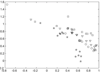
Fig. 2. Affine coordinates of four projective representations of facial landmarks.
Case II. The simultaneous confidence intervals for the coordinates (xk, yk), k ∈ {1, ...,4}of the four observations, non-symmetric about ˆσ2, forα= 0.05, γ= 0.045,
x1∈[−0.0134686026942806,0.139107857780284]
x2∈[−0.165255061513897,0.39784731336349]
x3∈[0.00823968853543718,0.0793537101121015]
x4∈[−0.0367704220678841,0.198104003255809]
y1∈[−0.0027070765829481,0.0307222756205941]
y2∈[−0.0802709180592805,0.211303466325924]
y3∈[0.0525130444845735,0.143946381906257]
y4∈[0.00258061045344363,0.0652571391577564].
If we select centered confidence intervals, at levelα= 0.05 we accept (fail to reject) the planarity of three of the four inner eye ends and nose ends, and reject it for three landmarks. If we are more inclusive for the lower bound of the confidence intervals, by takingγ= 0.045 then we reject the tip of the nose as being in the plane determined by the lines of the eyes and of the lip ends, which comes in agreement with our expectations.
Acknowledgement.The present work was supported by NSA-MSP-H98230-08-1-0058 (for the second and third author), by NSF-DMS-0805977 (for the third author), NSF DMS-0713012 (for the fourth author) and by the Romanian Academy Grant 5/5.02.2008 (for the first author).
References
[1] V. Balan, V. Patrangenaru,Geometry of shape spaces, Proc. of The 5-th Conference of Balkan Society of Geometers, August 29 - September 2, 2005 Mangalia, Romania, BSG Proceedings 13, Geometry Balkan Press, Bucharest 2006, 28-33.
[2] A. Bhattacharya, (2008).Statistical analysis on manifolds: A nonparametric approach for inference on shape spaces, Ann. Statist., 2008.
[3] R.N. Bhattacharya, V. Patrangenaru,Nonparametic estimation of location and disper-sion on Riemannian manifolds, Journal of Statistical Planning and Inference 108, 1-2 (2002), 23–35.
[4] R.N. Bhattacharya, V. Patrangenaru, Large sample theory of intrinsic and extrinsic sample means on manifolds-I, Ann. Statist. 31, 1 (2003), 1–29.
[5] R.N. Bhattacharya, V. Patrangenaru, Large sample theory of intrinsic and extrinsic sample means on manifolds- Part II, Ann. Statist. 33, 3 (2005), 1211–1245.
[6] B. Efron,Bootstrap methods: another look at the jackknife, Ann. Statist. 7, 1 (1979), 1–26.
[7] B. Efron,The Jackknife, the Bootstrap and Other Resampling Plans, CBMS-NSF Re-gional Conference Series in Applied Mathematics SIAM 38 (1982).
[8] C. Goodall, K.V. Mardia, Projective shape analysis, J. Graphical & Computational Statist. 8 (1999), 143–168.
[9] R.I. Hartley, R. Gupta R., T. Chang, Stereo from uncalibrated cameras, Proc. IEEE Conference on Computer Vision and Pattern Recognition, 1992.
[11] J.T. Kent, K.V. Mardia, A new representation for projective shape, in (Eds: S. Barber, P.D. Baxter, K.V.Mardia, & R.E. Walls) ”Interdisciplinary Statistics and Bioinformatics”, Leeds, Leeds University Press 2006, 75-78; http://www.maths.leeds.ac.uk/lasr2006/proceedings/
[12] J.L. Lee, R. Paige, V. Patrangenaru, F. Ruymgaart, Nonparametric den-sity estimation on homogeneous spaces in high level image analysis, in (Eds: R.G. Aykroyd, S. Barber, & K.V. Mardia) ”Bioinformatics, Images, and Wavelets”, Department of Statistics, University of Leeds 2004, 37-40; http://www.maths.leeds.ac.uk/Statistics/workshop/leeds2004/temp
[13] X. Liu, V. Patrangenaru, S. Sugathadasa,Projective Shape Analysis for Noncalibrated Pinhole Camera Views, Florida State University, Department of Statistics, Technical Report M983, 2007.
[14] Y. Mao, S. Soatto, J. Kosecka, S.S. Sastry,An invitation to 3-D Vision, Springer 2006.
[15] K.V. Mardia, V. Patrangenaru, Directions and projective shapes, Ann. Statist. 33, 4 (2005), 1666–1699.
[16] K.V. Mardia, C. Goodall, A.N. Walder,Distributions of projective invariants and model based machine vision, Adv. in App. Prob. 28 (1996), 641–661.
[17] S.J. Maybank,Probabilistic analysis of the application of the cross ratio to model based vision: Misclassification, Inter. J. of Computer Vision 14 (3) (1995).
[18] S.J. Maybank,Classification based on the cross ratio, in ”Applications of Invariance in Computer Vision”, Lecture Notes in Comput. Sci. 825 (Eds: J.L. Mundy, A. Zisserman and D. Forsyth), Springer, Berlin 1994, 433–472.
[19] A. Munk, R. Paige, J. Pang, V. Patrangenaru and F. Ruymgaart, The one and mul-tisample problem for functional data with applications to projective shape analysis, to appear in Journal of Multivariate Analysis, 99 (2009), 815-833.
[20] V. Patrangenaru,Moving projective frames and spatial scene identification, in Proceed-ings in Spatial-Temporal Modeling and Applications (Eds: K.V. Mardia, R.G. Aykroyd and I.L. Dryden), Leeds University Press 1999, 53–57.
[21] V. Patrangenaru,New large sample and bootstrap methods on shape spaces in high level analysis of natural images, Commun. Statist. 30 (2001), 1675–1693.
[22] V. Patrangenaru, X. Liu and S. Sugathadasa,Nonparametric 3D projective shape es-timation from pairs of 2D images - I, In Memory of W.P. Dayawansa, Journal of Multivariate Analysis (2009), in press.
Vladimir Balan
University Politehnica of Bucharest, Faculty of Applied Sciences, Department of Mathematics-Informatics I,
Splaiul Independentei 313, Bucharest 060042, Romania. E-mail: [email protected]
M. Crane, Victor Patrangenaru and X. Liu Florida State University, USA.