AN ANALYSIS OF GCD AND LCM MATRICES VIA THE
LDLT-FACTORIZATION∗
JEFFREY S. OVALL†
Abstract. LetS={x1, x2, . . . , xn}be a set of distinct positive integers such that gcd(xi, xj)∈
Sfor 1≤i, j≤n. Such a set is called GCD-closed. In 1875/1876, H.J.S. Smith showed that, if the set Sis “factor-closed”, then the determinant of the matrixeij= gcd(xi, xj) is det(E) =nm=1φ(xm), where φdenotes Euler’s Phi-function. Since the early 1990’s there has been a rebirth of interest in matrices defined in terms of arithmetic functions defined on S. In 1992, Bourque and Ligh conjectured that the matrix fij = lcm(xi, xj) is nonsingular. Several authors have shown that, although the conjecture holds forn≤7, it need not hold in general. At present there are no known necessary conditions forF to be nonsingular, but many have offered sufficient conditions.
In this note, a simple algorithm is offered for computing theLDLT-Factorization of any matrix bij = f(gcd(xi, xj)), where f : S → C. This factorization gives us an easy way of answering the question of singularity, computing its determinant, and determining its inertia (the number of positive negative and zero eigenvalues). Using this factorization, it is argued thatEis positive definite regardless of whether or notSis GCD-closed (a known result), and thatF is indefinite forn≥2. Also revisited are some of the known sufficient conditions for the invertibility ofF, which are justified in the present framework, and then a few new sufficient conditions are offered. Similar statements are made for the reciprocal matricesgij= gcd(xi, xj)/lcm(xi, xj) andhij= lcm(xi, xj)/gcd(xi, xj).
Key words. GCD and LCM matrices, Reciprocal GCD and LCM matrices, Determinants, Singularity, Inertia,LDLT-Factorization, Partially ordered sets.
AMS subjectclassifications. 06A07, 06A12, 11A05, 15A18, 15A23, 15A36.
1. Introduction. LetS={x1, x2, . . . , xn} be a set of distinct positive integers
which is GCD-closed, gcd(xi, xj) ∈ S for 1 ≤i, j ≤n. In 1992, Bourque and Ligh
[4] conjectured that the matrix fij = lcm(xi, xj) is nonsingular. Several authors
[5,6,7,12] have shown that, although the conjecture holds for n ≤ 7, it need not hold in general. At present there are no known necessary conditions for F to be nonsingular, but many have offered sufficient conditions ([6,12] for instance). In this paper, we address the question of singularity of the matricesfij = lcm(xi, xj)
and hij = lcm(xi, xj)/gcd(xi, xj) by looking at their LDLT-Factorizations, offering
several new sufficient conditions for nonsingularity. The paper is structured as follows:
• In section 2, we present an algorithm for finding the LDLT-Factorization
of any matrix of the form bij = f(gcd(xi, xj)), where f : S → C. This
factorization provides an easy way of answering the question of singularity ofB, computing its determinant, and determining its inertia (the number of positive negative and zero eigenvalues).
• In section 3, we show that both the GCD and reciprocal GCD/LCM matrices are positive definite (regardless of whether or notS is GCD closed) by em-bedding them in larger matrices which are shown to be positive definite by
∗Received by the editors 7 November 2003. Accepted for publication 11 February 2004. Handling
Editor: Daniel Hershkowitz.
†Department of Mathematics, University of California at San Diego, La Jolla, California
92093-0112, USA ([email protected]).
looking at theirLDLT-Factorizations. The LCM and reciprocal LCM/GCD
matrices are shown to be indefinite forn≥2.
• Section 4 contains several examples of sufficient conditions for the invertibility of LCM and reciprocal LCM/GCD matrices onS, culminating in an example that includes many of the sufficient conditions given in the literature as special cases, with the notable exception of H. J. Smith’s condition thatSbe factor-closed [10]. Many of the sufficient conditions presented here are described in terms of properties of the Hasse diagram associated withS.
2. The Factorization Theorem. Let P = {1,2, . . . , n} and be a partial ordering onP such that the greatest lower bound (with respect to ) of any pair of elements inP is defined and inP, glb(i, j)∈ P. Such a partially ordered set (poset), (P, ) is called a meet semi-lattice. We will assume here thati j impliesi≤j.
LetI denote the set of pairs of comparable elements inP,I ={(k, l)∈ P × P : k l}, and µ : I → Z denote the corresponding M¨obius function. We have the
following well-known variant of the M¨obius inversion formula.
Theorem 2.1 Form∈ P andg:P →C,
g(m) =
dm
cd
µ(c, d)g(c).
Remark 2.2 Under the partial orderingi j iffi|j, µ(c, d) =µ(d/c) where µ(·) is the M¨obius function from elementary number theory.
Recognizing that {d ∈ P : d glb(i, j)} = {d ∈ P : d iandd j}, we rephrase Theorem 2.1 as a statement about the factorization ofbij =g(glb(i, j)).
Theorem 2.3 [The Factorization Theorem] Let bij = g(glb(i, j)) and vg =
[g(1)g(2) . . . g(n)]T. Let LandM be given by
lid=
1 if d i
0 otherwise, mdj=
µ(j, d) if j d
0 otherwise.
Then B=LDLT, whereD=diag(M v g).
Remark 2.4 The factorization given above is similar to that given by Bhat [3].
Remark 2.5 The condition that g map into C is more restrictive than necessary.
We can takeg to map into any vector space overC (Cm×m for instance), and more
generally into any abelian group, although the usefulness of such generality is ques-tionable.
Remark 2.6 ThatLandMare inverses is a well-known consequence of the definition ofµ. In fact, in some treatmentsµis defined in terms of the inverse ofL.
We now use the factorization theorem to analyze matrices of the form bij =
question of singularity for the LCM and reciprocal LCM/GCD matrices. We define the partial ordering onP,i jiffxi|xj. Givenf :S→C, letg=f◦pwherep(k) =xk.
Note that p(glb(i, j)) = gcd(xi, xj). So we have that f(gcd(xi, xj)) = g(glb(i, j)),
and the factorization algorithm forbij=f(gcd(xi, xj)) follows immediately:
Algorithm 2.7 The Factorization Algorithm.
1. Form the vectorvf = [f(x1)f(x2) . . . f(xn)]T and the matrix
lij =
1 if xj|xi
0 otherwise.
2. Solve the (lower-triangular) systemLu=vf via forward substitution.
3. B=LDLT where D= diag(u).1
Corollary 2.8 We have det(B) = nm=1um and the number of positive, negative and zero eigenvalues of B (its inertia) is equal to the number of positive, negative, and zero entries ofu.
Remark 2.9 The assumption that S is GCD-closed is what made (P, ) a meet semi-lattice, and allowed this factorization.
3. Basic Results on Inertia. Let the matricesE, F, GandH be defined by
eij= gcd(xi, xj), fij = lcm(xi, xj), gij =
gcd(xi, xj)
lcm(xi, xj)
, hij =
lcm(xi, xj)
gcd(xi, xj)
.
The following result concerning the inertias ofE andG is well-known, being shown in [2] and [8] respectively (and elsewhere). We offer a different, simple proof based on the factorization algorithm.
Theorem 3.1 The matrices E and Gare positive definite, regardless of whether or notS is GCD-closed.
Proof. LetN =xn= maxS. The GCD matrixE is a principal submatrix of the
N×N matrixaij = gcd(i, j); so, if A is positive definite, then E is as well. Using
the factorization theorem onA, we deduce that its inertia is determined by the set of
numbers
d|mµ(m/d)d N
m=1={φ(m)}
N
m=1, which are clearly positive.
After recognizing that gij =
gcd(xi,xj)2
xixj and ˜gij = gcd(xi, xj)
2 have the same
inertia {G = KTGK,˜ forK = diag(1/x
1,1/x2, . . . ,1/xn)}, we can use the same
argument as above with ˜Gbeing a principal submatrix of theN ×N matrixaij =
gcd(i, j)2. Its inertia is determined by the set of numbers
d|mµ(m/d)d2 N
m=1,
which are also positive. We note that S did not have to be GCD-closed for this argument.
Analyzing the inertias ofF andH by embedding each in larger related matrices in the manner above fails because these larger matrices are indefinite, so they cannot
1We haveu
give us useful information about the inertias of their principal submatrices. We can see directly from the factorization algorithm, however, that
Theorem 3.2 The matrices F andH are indefinite forn≥2. Proof. Since
have the same inertias as
˜
respectively, we need merely consider the two systemsLu=v1 and Lw=v2, where
v1= [1/x11/x2· · ·1/xn]T andv2= [1/x211/x22· · ·1/x2n] T.
Regardless of the partial ordering that divisibility induces onS, we can be certain that the first two equations in the systems are
u1=
4. Some Sufficient Conditions for the Invertibility ofF andH. We have seen that inertias ofF andH are the same as those of ˜F and ˜H, so we need merely consider the systemsLu = v1 and Lw =v2, where v1 = [1/x1 1/x2· · ·1/xn]T and
v2= [1/x211/x22· · ·1/x2n]T, to determine whether or notF andH are nonsingular. In
particular, they will be nonsingular if and only if the solutionsuandwhave no zero components. Below, we give several examples of sufficient conditions for invertibility ofF andH. We only explicitly treat F, but the arguments are easily adapted forH as well - we need only replace 1/xi by 1/x2i in each of the equations and inequalities.
Example 4.3 S has the property thatx1|x2| · · · |xn. The equations to solve here are
We note here that the only elements inSwhich have any bearing on the componentuk
of the systemLu=vf are those which dividexk. So we can, for purposes of analysis,
decouple the larger system into several smaller ones - one for each of the maximal elements ofS. We use this fact to demonstrate another set of sufficient conditions for the invertibility ofF andH which generalizes those offered in Examples 4.2 and 4.3.
Example 4.4 The Hasse diagram forS is a tree. We can see this by decoupling the corresponding system of equations into several systems of the form in Example 4.3 - one for each of the maximal chains in S (the fact that a given xj might belong to
more than one chain is irrelevant). We already saw that the solution of such systems is completely nonzero.
Example 4.5 S has the property that gcd(xi, xj) =x1for 2≤j ≤n−1
andx1|xj|xn for 1 ≤j ≤n. The case n = 3 is trivial, so we assume n > 3. The
equations to solve here are
u1= 1/x1, u1+uj = 1/xj for 2≤j≤n−1 and ni=1ui= 1/xn.
It is clear that the only equation we have to be concerned about is the last one, where we solve forun. We have
chain. This is an extension of Example 4.5 and can be analyzed in the same way. As in example 4.5, we need only be concerned about un. Letyj denote the second
largest element (afterxn) inCj. We have
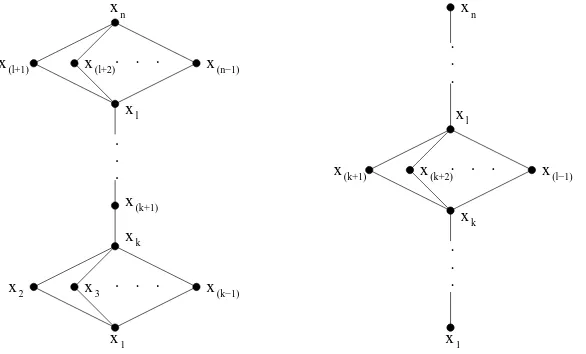
x
1Fig. 4.1.Example 4.2 (left) and 4.5 (right).
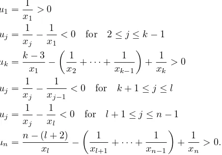
Example 4.7 Any set S for which the associated Hasse diagram is given in Figure 4.2 (left). The solutionuof the associate system is
u1=
Example 4.8 Any set S for which the associated Hasse diagram is given in Figure 4.2 (right). The solutionuof the associate system is
u1= 1
n x
. . .
x1 . . . l x
(k−1) 3
2
1
x x
x
k x
(k+1) x(k+2). . . x(l−1)
x
l x (l+1)
x
. . .
(k+1) x
k x
x . . .
(n−1) n
(l+2)
x x
x
. . .
Fig. 4.2.Example 4.7 (left) and 4.8 (right).
chain, and replacing one or two vertices with a simple bulb in the ways shown in Figure 4.2. It is a trivial extension of these examples to recognize that any set S whose Hasse diagram can be constructed from a single maximal chain by replacing some of the vertices with simple bulbs gives rise to nonsingular matricesF and H. Actually, one could replace some of the vertices with general bulbs instead without affecting the singularity ofF and H. We shall call such a Hasse diagram a “burled chain”. These examples and discussion serve as lemmas for our final example, which generalizes all of the previous ones except for Smith’s example (4.1).
Example 4.9 Any set S for which the associated Hasse diagram which can be con-structed by beginning with a tree, and then replacing some of the vertices with general bulbs, thereby creating a “burled tree”. We can decouple the associated system of equations into several smaller systems associated with the maximal “burled chains”. As the previous two examples suggest, these systems have solutions which are com-pletely nonzero.
REFERENCES
[1] J. Scott Beslin. Reciprocal GCD matrices and LCM matrices. The Fibonacci Quarterly, 29(3):271–274, 1991.
[2] J. Scott Beslin and Steve Ligh. Greatest common divisor matrices. Linear Algebra and its Applications, 118:69–76, 1989.
[3] B.V. Rajarama Bhat. On greatest common divisor matrices and their applications. Linear Algebra and its Applications, 158:77–97, 1991.
[4] Keith Bourque and Steve Ligh. On GCD and LCM matrices. Linear Algebra and its Appli-cations, 174:65–74, 1992.
[5] P. Haukkanen, J. Sillanp¨a¨a, and J. Wang. On Smith’s determinant. Linear Algebra and its Applications, 258:251–269, 1997.
[6] S. Hong. On LCM matrices on GCD-closed Sets. Southeast Asian Bulletin of Mathematics, 22:381–384, 1998.
[7] S. Hong. On the Bourque-Ligh conjecture of least common multiple matrices. Journal of Algebra 218(1):216–228, 1999.
[8] P. Lindquist and K. Seip. Note on some greatest common divisor matrices.Acta Arithmetica, 82(2):149–154, 1998.
[9] H. Montgomery, I. Niven, and H. Zuckerman.An Introduction to the Theory of Numbers, 5th Ed., pp. 193–197. John Wiley & Sons, Inc., New York, 1991.
[10] H.J.S. Smith. On the value of a certain arithmetical determinant.Proceedings of the London Mathematical Society: 7:208–212, 1875-1876.
[11] R.P. Stanley.Enumerative Combinatorics, Volume 1, Ch. 3. Advanced Books and Software, Wadsworth & Brooks/Cole, Monterey, CA, 1986.