Full Terms & Conditions of access and use can be found at
http://www.tandfonline.com/action/journalInformation?journalCode=ubes20
Download by: [Universitas Maritim Raja Ali Haji] Date: 11 January 2016, At: 18:54
Journal of Business & Economic Statistics
ISSN: 0735-0015 (Print) 1537-2707 (Online) Journal homepage: http://www.tandfonline.com/loi/ubes20
Simulation-Based Density Estimation for Time
Series Using Covariate Data
Yin Liao & John Stachurski
To cite this article: Yin Liao & John Stachurski (2015) Simulation-Based Density Estimation for Time Series Using Covariate Data, Journal of Business & Economic Statistics, 33:4, 595-606, DOI: 10.1080/07350015.2014.982247
To link to this article: http://dx.doi.org/10.1080/07350015.2014.982247
Published online: 27 Oct 2015.
Submit your article to this journal
Article views: 87
View related articles
Simulation-Based Density Estimation for Time
Series Using Covariate Data
Yin LIAO
School of Economics and Finance, Queensland University of Technology, Brisbane, QLD 4000, Australia ([email protected])
John STACHURSKI
Research School of Economics, Australian National University, Canberra, ACT 0200, Australia ([email protected])
This article proposes a simulation-based density estimation technique for time series that exploits infor-mation found in covariate data. The method can be paired with a large range of parametric models used in time series estimation. We derive asymptotic properties of the estimator and illustrate attractive finite sample properties for a range of well-known econometric and financial applications.
KEY WORDS: Density estimation; Simulation.
1. INTRODUCTION
In this article, we study a parametric density estimation tech-nique for time series that exploits covariate data. While the technique has broad applicability, our motivation stems from applications in econometrics and finance where density estima-tion is often used for tasks such as analysis of asset returns, interest rates, GDP growth, inflation and so on. For example, the Bank of England routinely estimates densities for inflation and a wide range of asset prices using options data (de Vincent-Humphreys and Noss2012). In settings such as this, the primary attraction of density estimates is that they typically provide more information than estimates of central tendency or a finite set of moments. Depending on the time series in question, density estimates can be used to address a large variety of questions, such as the risk of corporate (or sovereign) default, or the like-lihood of recession, or of inflation leaving a target band over a given interval of time. For related applications and discussion, see, for example, A¨ıt-Sahalia and Hansen (2009), Calabrese and Zenga (2010), or Polanski and Stoja (2011). In addition to situa-tions where the density itself is of primary interest (e.g., density forecasting), density estimation is also used in a wide range of statistical techniques where density estimates are an input, such as discriminant or cluster analysis. Similarly, density estima-tors are used to address specification testing or model validation problems (e.g., A¨ıt-Sahalia, Fan, and Peng2009).
A variety of techniques for estimating densities has been proposed in the literature. One popular approach is nonpara-metric kernel density estimation (Rosenblatt1956). Nonpara-metric density estimators have an advantage over paraNonpara-metric methods in terms of robustness and generality, in the sense that asymptotic convergence occurs under very weak assumptions. This makes nonparametric density estimators ideal for certain applications, particularly those where the risk of model mis-specification is high.
On the other hand, for some of the more common eco-nomic and financial time series, econometricians have spent decades formulating, developing, and testing parametric time series models (e.g., autoregressive moving average (ARMA)
models, generalized autoregressive conditional heteroskedas-ticity (GARCH) models and their many variations, Markov switching models, stochastic volatility models, dynamic fac-tor models, threshold models, etc.). This research has generated a very substantial body of knowledge on classes of parametric models and how they can be paired with certain time series to effectively represent various data-generating processes (for a recent overview, see Martin, Hurn, and Harris2012). In these kinds of settings, it is natural to seek techniques that can exploit this parametric information to construct density estimators. Our article pursues this idea, with the focus on providing a flexible density estimation scheme that can be used in combination with common time series models.
In doing so we confront several problems associated with these kinds of estimation. First, many modern econometric models have nonlinear or non-Gaussian features that make the relevant densities intractable. Hence, generating density esti-mates requires some form of approximation. Second, time se-ries datasets are often (a) smaller than cross-sectional datasets, and (b) contain less information for a given data size, since observations are more likely to be correlated. This problem of information scarcity is compounded in the case of density esti-mation, since the “point” we are trying to estimate is, in general, an infinite-dimensional object.
The technique we study addresses these problems simultane-ously. To accommodate the problem that the densities might be intractable, we use a simulation-based approach, which permits construction of density estimates from model primitives in a wide range of settings. To address the issue of limited data, we combine two useful ways to supplement the amount of infor-mation available for estiinfor-mation of a given density: exploitation of parametric structure and incorporation of information from
© 2015American Statistical Association Journal of Business & Economic Statistics October 2015, Vol. 33, No. 4 DOI:10.1080/07350015.2014.982247 Color versions of one or more of the figures in the article can be found online atwww.tandfonline.com/r/jbes.
595
covariates. (The meaning of the second point is as follows: Sup-pose that we wish to estimate the densityf of a random vector
Yt. One possibility is to use only observations ofYt. If, however,
we possess a model that imposes structure on the relationship betweenYtand a vector of covariatesXt, we can use this
struc-ture and additional data to improve our estimate off.) Our article pursues these ideas within a parametric time series setting. Our simulation studies give a number of examples as to how inclu-sion of parametric structure combined with covariate data can greatly reduce mean squared error.
From a technical perspective, the method we study in this article can be understood as a variation on conditional Monte Carlo (see, e.g., Henderson and Glynn2001), which is an elegant and effective technique for reducing variance in a variety of Monte Carlo procedures. Here the estimation target is a density. In addition, the primitives for the simulation contain estimated parameters. Accommodating this randomness together with the randomness introduced by the Monte Carlo step, we establish a functional central limit result for the error of the estimator. The theorem also shows that the estimated density converges to the target density in mean integrated squared error.
Following presentation of the theory, we turn to illustrations of the method for a variety of econometric and financial appli-cations, and to Monte Carlo analysis to investigate finite sample behavior. The case studies include dynamic factor models, linear and nonlinear autoregressive models, Markov regime switching models, and stochastic volatility models. In all cases, the method exhibits excellent finite sample properties. We give several in-terpretations of this performance.
Regarding related literature, alternative parametric density estimators using covariates were proposed by Saavedra and Cao (2000) and Schick and Wefelmeyer (2004,2007) for linear pro-cesses, by Frees (1994) and Gine and Mason (2007) for functions of independent variables, by Kim and Wu (2007) for nonlin-ear autoregressive models with constant variance, and by Støve and Tjøstheim (2012) for a nonlinear heterogenous regression model. A related semiparametric approach was proposed by Zhao (2010). In addition, Escanciano and Jacho-Ch´avez (2012) exhibited a nonparametric estimator of the density of response variables that is√n-consistent. Our setup is less specific than the parametric treatments discussed above. For example, we make no assumptions regarding linearity, additive shocks, con-stant variance and so on, and the density of interest can be vector valued. A Monte Carlo step makes the method viable despite this generality. On the other hand, relative to the nonparametric and semiparametric methods, our estimator puts more emphasis on finite sample properties. These points are illustrated in depth below.
The structure of our article is as follows: Section 2 gives an introduction to the estimation technique. Section3provides asymptotic theory. Section4looks at a number of applications and provides some Monte Carlo studies. Section 5 discusses robustness issues. Section6gives proofs.
2. OUTLINE OF THE METHOD
Our objective is to estimate the densityf of random vector
Yt. To illustrate the main idea, suppose that, in addition to the
original dataY1, . . . , Yn, we also observe a sequence of
covari-atesX1, . . . , Xn, where{Xt}is a stationary and ergodic
vector-valued stochastic process. Suppose further thatYt is related to
XtviaYt|Xt ∼p(· |Xt). That is,p(· |x) is the conditional
den-sity ofYt givenXt =x. Since {Xt}andp are assumed to be
stationary, the target process{Yt}is likewise stationary. Letting
φbe the common stationary (i.e., unconditional) density ofXt,
an elementary conditioning argument tells us that the densities f andφare related to one another by
f(y)=
p(y|x)φ(x)dx (y ∈Y). (1)
Example 2.1. Suppose that Yt denotes returns on a given
asset, and let{Yt}obey the GARCH(1,1) modelYt =μ+σtǫt,
where {ǫt}is iid and N(0,1), andσt2+1=α0+α1σt2+α2Yt2.
Assume all parameters are strictly positive and α1+α2<1. LetXt:=σt2, so that
Xt+1=α0+α1Xt+α2(μ+
Xtǫt)2. (2)
Letφbe the stationary density of this Markov process. In this setting, (1) becomes
f(y)=
∞
−∞ 1
√
2π xexp
−(y−μ)
2
2x
φ(x)dx. (3)
Returning to the general case, suppose for the moment that the conditional densitypisknown. Given observations{Xt}nt=1, there is a standard procedure for estimatingf called conditional density estimation that simply replaces the right-hand side of (1) with its empirical counterpart
ˆ
r(y) :=n1
n
t=1
p(y|Xt). (4)
Since{Xt}is assumed to be ergodic with common marginalφ,
the law of large numbers and (1) yield
ˆ
r(y)= 1
n
n
t=1
p(y|Xt)→
p(y|x)φ(x)dx=f(y)
as n→ ∞. A more complete asymptotic theory is provided in Braun, Li, and Stachurski (2012). (The assumption that p is known is appropriate in a computational setting, where all densities are known in principle butf might be intractable and hence require estimation (in the sense of approximation via Monte Carlo). This is the perspective taken in Gelfand and Smith (1990), Henderson and Glynn (2001), Braun, Li, and Stachurski (2012) and many other articles. The asymptotic theory is well established.)
In a statistical setting, the conditional densitypis unknown. If we are prepared to impose parametric assumptions, then we can write
Yt|Xt∼p(· |Xt, β), (5)
where β is a vector of unknown parameters. In this case, an obvious extension to (4) is to replace the unknown vector β
with an estimate ˆβn obtained from the data {Yt, Xt}nt=1. This
leads to the semiparametric estimator
ˆ
s(y) := 1
n
n
t=1
p
y|Xt,βˆn. (6)
The estimator is semiparametric in the sense that if we letφnbe
the empirical distribution of the sampleX1, . . . , Xn, then ˆscan
be expressed as
ˆ
s(y)=
py|x,βˆn
φn(dx). (7)
Thus, ˆs combines the parametric conditional density estimate
p(· | ·,βˆn) with the nonparametric empirical distributionφn to
obtain an estimate of f. The random density ˆs is known to be consistent and asymptotically normal for f under certain regularity conditions (Zhao2010, Theorem 1).
While this semiparametric estimator ˆsis natural, there are a number of settings where it cannot be applied, or where its finite sample performance is suboptimal. As a first example, consider a setting where we have a parametric model for the dynamics of {Xt} that provides an accurate fit to this data. In such a
setting, these estimated dynamics allow us to produce a good estimate for the stationary densityφof{Xt}. The semiparametric
estimator ˆsfails to exploit this knowledge, replacing it with the (nonparametric) empirical distributionφn.
Another example along the same lines is a setting such as
Yt =β′Xt+σ ǫt, whereXt =(Yt−1, . . . , Yt−p). Here, the
co-variates are just lagged values of the current state. If we estimate (β, σ), then we can in fact deduce the stationary density φof
Xt coinciding with this estimate. It would be inconsistent to
discard this stationary density and use the empirical distribution
φninstead.
In addition to the above, there are settings where the semi-parametric estimator cannot be used at all. For example, many time series models incorporate latent variables (e.g., latent state space, latent factor and hidden Markov models, regime switch-ing models, GARCH models, and stochastic volatility models). In all these models, the process{Xt}is not fully observable, and
hence the semiparametric estimate ˆsin (6) cannot be computed. As we now show, all of these issues can be addressed in a set-ting where we are prepared to add more parametric structure— in particular, parametric information about the process{Xt}. In
what follows, this parametric information is assumed to take the form
Xt+1|Xt ∼q(· |Xt, γ), (8)
whereγ is another vector of unknown parameters. (Although we are restricting the model to a first-order process, this costs no generality, since anyp-order process can be reduced to a first-order process by reorganizing state variables.)
Given this information, to estimatef, the procedure we con-sider is as follows:
1. Estimate the parameters in (5) and (8) with ˆβnand ˆγn,
re-spectively. 2. Simulate{X∗
t} m t=1via
X∗t+1∼q(· |X∗t,γˆn) with X∗0=x. (9)
3. Return the function ˆf defined by
ˆ
f(y) := 1
m
m
t=1
p(y|Xt∗,βˆn). (10)
In what follows, we refer to the estimator ˆf in (10) as the parametric conditional Monte Carlo(PCMC) density estimator. Comparing ˆsdefined in (6) with the PCMC density estimator ˆf, the difference is that while ˆsuses the observed data{Xt}directly
on the right-hand side of (6), the PCMC density estimator uses simulated data instead. More precisely, instead of using {Xt}
directly, we use{Xt}to estimate the model (8), and then use that
model to generate simulated data{Xt∗}.
Example 2.1 (continued) Consider again the GARCH model presented in example 2.1. Let ˆθ:=( ˆμ,αˆ0,αˆ1,αˆ2) be a consis-tent estimator of the unknown parameters. By plugging these estimates into (2), we simulateX∗
1, . . . , Xm∗. Recalling (3), the
PCMC density estimator is then
ˆ
f(y)= m1
m
t=1 1
2π X∗
t
exp
−(y−μˆ)
2
2X∗
t
. (11)
2.1 Discussion
One attractive feature of the PCMC density estimator is that in a single simulation step, it bypasses two integration problems that in general fail to have analytical solutions. Without simula-tion, we would need to (a) take the estimated transition density
q(x′|x,γˆ
n) and calculate from it the corresponding
station-ary distributionφ(·,γˆn) as the solution to an integral equation,
and then (b) calculatefas p(y|x,βˆn)φ(x,γˆn)dx. Apart from
some special cases, neither of these integration problems can be solved in closed form.
Two other attractive features of ˆf are as follows: First, the initial valuexin (9) can be chosen arbitrarily. This is significant because, as discussed immediately above, the stationary density
φ(·,γˆn) is typically intractable, and we have no way to sample
from it directly. In Section3, we prove that our convergence re-sults do not depend on the choice ofx. Second, latent variables in
{Xt}cause no difficulties in using the PCMC density estimator.
As soon as we estimate the transition densityq(x′|x,γˆn), we can
produce the simulated data{X∗
t}. In this simulated data, latent
variables become observable. (A simulation-based method for density estimation in the context of parametric time series mod-els with latent states is also considered in Zhao (2011). Zhao’s estimator requires a significantly more complex formula, in-volving the ratio of empirical estimates of a joint and a marginal density. However, this additional complexity arises because he aimed to estimate a family of conditional densities providing all the dynamics of the hidden state vector, which can then be tested via a simultaneous confidence envelope constructed us-ing nonparametric methods. In contrast, the PCMC estimates a single density, and we provide a detailed asymptotic theory for that estimate.)
On the other hand, when comparing ˆsand ˆf in (6) and (10), respectively, the fact that the latter uses simulated data from an estimated model instead of observed data clearly involves some cost. When interpreting this difference, however, it is helpful to
−0.10 −0.08 −0.06 −0.04 −0.02 0 0.02 0.04 0.06 0.08 0.1 5
10 15 20 25
S&P500 S&P600
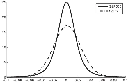
Figure 1. Estimated return densities, small cap versus large cap.
bear in mind that in a sense both techniques do use the observed data. What differs is the way in which these data are used. While the semiparametric estimator ˆs uses{Xt}to construct
an empirical distribution (φn on the right-hand side of (7)),
the PCMC uses this data to estimate a parametric model. To the extent that the parametric assumptions are correct, this approach can translate into better finite sample properties. These ideas are addressed in Section4via a range of simulation studies. At the same time, to quantify the estimation effect, we also include information on the errors associated with both ˆf and a version of ˆf called ˆf0that simulates from the exact model.
Figure 1 gives an example implementation of the PCMC
density estimator. In this application, we estimate two densities: the density of monthly returns on the S&P 500, a stock market index of 500 large companies listed on the NYSE or NASDAQ, and returns on the S&P 600, which is an index of smaller firms. Both densities are estimated using price data from January 2005 to December 2012. The model applied here is the GARCH model of Example 2.1. Volatility is latent in this model, but, as discussed above, this presents no difficulty for our procedure.
In interpreting the results, recall that small cap stocks usually have higher average returns than large cap stocks—for example, they are one of the three factors in the Fama-French three fac-tor model. Higher returns are typically associated with higher volatility, since the former is demanded as compensation for the latter by investors. Our estimates conform to this theory. (The mean of the density for the S&P 500 is 0.0006, while that for the S&P 600 is 2.8 times larger.)
2.2 Other Estimators
We have already mentioned several alternatives to the PCMC density estimator. There are several other parametric estima-tors off that could be considered here. One is to simply spec-ify a parametric class{f(·, θ)}θ∈ forf, estimateθ using{Yt}
and plug in the result ˆθ to produce ˆf :=f(·,θˆ). (e.g., specify
f =N(μ, σ) and plug in the sample mean ˆμ and the sample standard deviation ˆσ.) We refer to this estimator as the ordinary parametric estimator (OPE). In finite samples, this estimator is typically inferior to the PCMC density estimator because it fails to exploit the information available in covariates. Section4gives an extensive discussion of this point.
A parametric density estimator thatdoesexploit covariate data can be obtained by (i) specifying a parametric formφ(x, γ) for
the common density ofXt, (ii) estimatingβ in (5) andγ in the
densityφ(x, γ) as ˆβnand ˆγn, and (iii) returning
ˆ
z(y) :=
p(y|x,βˆn)φ(x,γˆn). (12)
This estimator is impractical, since it involves integration prob-lems that are not generally tractable. It also has another less obvious deficiency: In contrast to the PCMC density estimator
ˆ
f, parametric specification is placed directly on the densityφof
Xt, rather than on the dynamic model (8). As a result, ˆztypically
fails to exploit the order information in{Xt}. This can be costly,
particularly when{Xt}is highly persistent. Sections4.1and4.2
elaborate, comparing ˆzand ˆf in simulation experiments across a variety of common models.
3. ASYMPTOTIC THEORY
In this section, we clarify assumptions and provide conver-gence results for the PCMC density estimator introduced in Section2.
3.1 Preliminaries
In this section, it will be convenient to letθ ∈be a vector containing all unknown parameters. Thusp(· |x, β) in (5) now becomesp(· |x, θ), whileq(· |x, γ) in (8) becomesq(· |x, θ). The setis taken to be a subset ofRK. Letθ
0represent the true value of the parameter vectorθ. It follows that the true density of
Ytis given byf(y, θ0) := p(y|x, θ0)φ(x, θ0)dx. To simplify
notation, in the sequel we let
dk(x, y, θ) :=φ(x, θ)
∂
∂θk
p(y|x, θ)+p(y|x, θ) ∂
∂θk
φ(x, θ),
whenever the derivatives exist. In particular,d(x, y, θ) is theK -vector obtained by differentiatingp(y|x, θ)φ(x, θ) with respect toθ, holdingxandyconstant.
Below we present an approximateL2 central limit theorem for the deviation between the PCMC density estimator ˆfand the true densityf(·, θ0). We take the setYin whichYttakes values
to be a Borel subset ofRd, and the symbolL2(Y) represents the set of (equivalence classes of) real-valued Borel measur-able functions onYthat are square-integrable with respect to Lebesgue measure. As usual, we set g, h:= g(y)h(y)dy, andg:=√ g, g.
A random element W taking values in L2(Y) is called centered Gaussian if h, W is zero-mean Gaussian for all
h∈L2(Y). Equivalently,W is centered Gaussian if its charac-teristic functionψ(h)=Eexp{i h, W} has the formψ(h)=
exp{− h, Ch/2} for some self-adjoint linear self-map C on
L2(Y).Cis called the covariance operator ofW. The operatorC satisfies g, Ch:=Eg, W h, Wfor allg, h∈L2(Y). Co-variance operators are themselves often defined by coCo-variance functions. To say thatκis the covariance function for covariance operatorCis to say thatCis defined by
g, Ch = κ(y, y′)g(y)h(y′)dydy′ (13)
for all g, h∈L2(Y). Further details on Hilbert space valued random variables can be found in Bosq (2000).
To prove the main result of this section, we require some dif-ferentiability and ergodicity assumptions. Our difdif-ferentiability assumption is as follows:
Assumption 3.1.There exists an open neighborhoodUof the true parameter vectorθ0and a measurable functiong:X×Y→R such that
1. gsatisfies
g(x, y)dx2
dy <∞,
2. θ →p(y|x, θ) andθ→φ(x, θ) are continuously differen-tiable overUfor all fixed (x, y)∈X×Y, and
3. d(x, y, θ) satisfies supθ∈Ud(x, y, θ)E≤g(x, y) for all
(x, y)∈X×Y.
In Assumption 3.1, the symbol · Eis the Euclidean norm
onRK. The subscript Eis used to differentiate the Euclidean
norm from theL2norm · .
The set in which Xt takes values will be denoted byX, a
Borel subset ofRJ. Regarding the process for
{Xt}defined in
(8), we make the following assumptions:
Assumption 3.2. For eachθ∈, the transition densityx′→
q(x′|x, θ) is ergodic, with unique stationary density φ(·, θ). Moreover, there exist a measurable functionV :X→[1,∞) and nonnegative constantsa <1 andR <∞satisfying
sup |h|≤V
h(x′)qt(x′|x, θ)dx′−
h(x′)φ(x′, θ)dx′
≤
atRV(x) as well as a function ρ ∈L2(Y) such that p(y|x, θ)≤
ρ(y)V(x)1/2for ally ∈Y,x ∈X,θ∈, andt ∈N.
The main content of Assumption 3.2 is that the process{Xt}
is always V-uniformly ergodic. This is a standard notion of ergodicity, and it generates enough mixing to yield asymptotic normality results under appropriate moment conditions. (The last part of Assumption 3.2 is just a moment condition.) It applies to many common time series models under standard stationarity conditions. Details can be found in Meyn and Tweedie (2009, chap. 16).
3.2 Results
We now study the deviation between the true densityf = f(·, θ0) and the PCMC density estimator ˆfm(·,θˆn) defined in
Section2. Since altering the values of densities at individual points does not change the distribution they represent, we focus on global error, treated as an element ofL2(Y). The latter is a natural choice, since the expectation of the squared norm of the error is then mean integrated squared error (MISE).
To state our main result, suppose now that the sequence of estimators {θˆn} is asymptotically normal, with √n( ˆθn−θ0)
d
→N(0,) for some symmetric positive definite =(σij). The simulation
sizemfor ˆfm(·,θˆn) is taken to beτ(n) whereτ :N→Nis a
given increasing function. In this setting, we have the following result:
Theorem 3.1. If Assumptions 3.1–3.2 are valid and
τ(n)/n→ ∞, then
√
n{fˆτ(n)(·,θˆn)−f(·, θ0)} d
→W (n→ ∞), (14)
whereWis a centered Gaussian inL2(Y) with covariance func-tion
κ(y, y′) := ∇θf(y, θ0)⊤∇θf(y′, θ0). (15)
Here∇θf(y, θ0) represents the vector of partial derivatives
∂f(y, θ0)/∂θk. Thus, the asymptotic variance of the density
es-timator reflects the variance in the parameter estimate ˆθn
trans-ferred via the slope of the density estimate with respect to the parameters in the neighborhood of the true parameter. A proof of Theorem 3.1 can be found in Section6.
In interpreting Theorem 3.1, it is useful to note thatκ(y, y′) is in fact the pointwise asymptotic covariance of the function on the left-hand side of (14) evaluated atyandy′. In particular,
κ(y, y) is the pointwise asymptotic variance aty, in the sense that, for ally ∈Y,
√
n{fˆτ(n)(y,θˆn)−f(y, θ0)} d
→N(0, κ(y, y)) (n→ ∞).(16) A consistent estimator for κ(y, y) is κˆ(y, y) := ∇θf(y,θˆn)⊤ˆ ∇θf(y,θˆn), where ˆ is a consistent
esti-mator of.
One way to understand (16) is to consider an ideal set-ting where all integrals have analytical solutions. In this case, we can take the same estimator ˆθn and plug it directly into
f(y, θ). A simple application of the delta method tells us that the asymptotic variance of this estimator f(y,θˆn) is
∇θf(y, θ0)⊤∇θf(y′, θ0), which is the same value κ(y, y)
obtained by the PCMC estimator. Thus, the PCMC estimator obtains the same asymptotic variance as the ideal setting, pro-vided that the simulation sample size grows sufficiently quickly withn.
Example 3.1. As a simple illustration where integrals are tractable, suppose we observe a sequence{Yt}nt=0from the AR(1) model
Yt=θ Yt−1+ξt, {ξt}
IID
∼ N(0,1). (17) To estimate the stationary densityf ofYtvia the PCMC
den-sity estimator we take Xt :=Yt−1, so thatYt=θ Xt+ξt, and
hence p(y|x, θ)=N(θ x,1). Let ˆθn be the least-square
esti-mate ofθ. Given this estimate we can construct the simulated sequence{X∗
t}by iterating onX∗t+1=θˆnX∗t +ξt∗. Taking that
data and averaging over the conditional density as in (10) pro-duces the PCMC density estimator. Regarding its asymptotic variance, note that both Xt andYt share the same stationary
density, which in this case isf(·, θ)=N(0,1/(1−θ2)). Also, the asymptotic variance of the ordinary least-square (OLS) es-timator ˆθnin this setting is 1/EXt2, which is 1−θ2. Applying
(15) and (16), the asymptotic variance of ˆfτ(n)(y,θˆn) is therefore
f′
θ(y, θ0)2(1−θ
2 0).
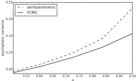
Figure 2compares the pointwise asymptotic variance of the
PCMC density estimator with that of the semiparametric esti-mator (6) when the model is the AR(1) process from Example 3.1. The comparison is across different values ofθwhile holding the pointyfixed (y =0 in this case). The asymptotic variance of the PCMC density estimator is lower at all points. The reason is that the simulation can almost eliminate the variance asso-ciated with averaging the conditional density over observations
Figure 2. Asymptotic variances in the AR(1) model.
of the covariateX. This dominates the estimation effect associ-ated with averaging over simulassoci-ated rather than actual data. (The comparison is by simulation to facilitate computation of the asymptotic variance of the semiparametric estimator. The sim-ulation is over 1000 replications withn=5000 and simulation size for the PCMC estimator set to 100,000.)
Example 3.2. We can also estimate f(y, θ) for the same AR(1) model via the estimator ˆz(y) in (12). Since the para-metric form in (17) is known here, it can be inferred that the stationary densityφ(·, θ) ofXtis the zero-mean Gaussian
distri-butionN(0,1/(1−θ2)). We can estimate the unknown variance from{Xt}with the sample variances2n. We can then back out
an estimate ¯θnofθ by solving 1/(1−θ2)=sn2forθ and then
plugging this into φ(y, θ). Next we compute the integral on the right-hand side of (12) to produce an estimate f(y,θ¯n).
Regarding the asymptotic variance, some elementary analysis shows that the asymptotic variance of ¯θnis (1−θ02)ζ, where
ζ :=1+(1−θ2
0)/(2θ02). Applying the delta method gives the asymptotic variance of f(y,θ¯n) as fθ′(y, θ0)2(1−θ2)ζ. Since
ζ >1, the pointwise asymptotic variance is larger than that of the PCMC (see Example 3.1). The intuition for this was dis-cussed in Section2.2.
4. SIMULATIONS
Next we apply the PCMC density estimator to a number of common models and examine its finite sample performance using Monte Carlo. In all cases, performance is measured in terms of mean integrated squared error (MISE). (The MISE of an estimator ˆg of the true density f =f(·, θ0) is Egˆ−
f2. Iff has no closed form solution, then we compute it by conditional Monte Carlo. In all the following simulations, the MISE is approximated by averaging 1000 realizations ofgˆ−
f2.)
4.1 Dynamic Factor Models
We begin with a simple application intended to illustrate conceptual issues. Consider the linear dynamic factor model
Yt=β⊤Xt+ξtwith
Xt+1=ŴXt+ηt+1. (18)
HereYt∈R,Xt∈R3,Ŵ=diag(γ1, γ2, γ3), and all shocks are independent andN(0,1). Following the asset pricing analysis
of He, Huh, and Lee (2010), our baseline parameter setting isβ1=6.26,β2=1.32,β3= −1.09,γ1=0.18,γ2 = −0.14, and γ3 =0.21. Using simulation, we compute the MISE of various estimators of the densityf ofYt. In this case, the true
density is equal to
f =N(0, σ2) for σ2:= β
2 1 1−γ12 +
β2 2 1−γ22+
β2 3 1−γ32 +1.
(19)
To investigate how the performance of the estimator changes with the degree of persistence in the data, we also consider variations from the baseline. In particular, the baseline values ofγ =(γ1, γ2, γ3) are multiplied by a scale parameterα, where
αvaries from 1 to 4. In all simulations, we take the data size
n=200.
To compute the PCMC density estimator ˆf from any one of these datasets{Yt, Xt}, we first estimateβandγby least squares,
producing estimates ˆβnand ˆγn. Next,{Xt∗} m
t=1 is produced by simulating from the estimated version of (18), starting atX0∗=0 and settingm=10,000. We then apply the definition (10) to obtain
ˆ
f(y)= 1
m
m
t=1 1
√
2π exp
−1
2
y−βˆn⊤X∗t2
.
For comparison, we also compute the MISE of four alternative estimators: the semiparametric estimator ˆsdefined in (7), ˆz de-fined in (12), the ordinary parametric estimator (OPE), and the nonparametric kernel density estimator (NPKDE), all of which are discussed earlier. The OPE uses the dynamic factor model to infer that (19) holds, and estimatesf asN(0,σˆ2
n) where ˆσ is
the sample standard deviation of{Yt}. The NPKDE uses a
stan-dard Gaussian kernel and Silverman’s rule for the bandwidth. To investigate the estimation effect, we also compute the PCMC density estimator with the true values ofβandγ, and label it as
ˆ
f0. See the discussion in Section2.1.
The results of the simulation are shown inTable 1. The far left-hand column is values of the scaling parameterα, so that higher values ofα indicate more persistence in{Xt}. The remaining
columns show MISE values for the six density estimators men-tioned above. All are expressed as relative to the PCMC density estimator ˆf (i.e., as multiples of this value). (Actual values for
ˆ
f ranged from 4.606×10⁻⁴to 5.182
×10−4.)
Regarding the outcome, observe that the rank of these esti-mators in terms of MISE is invariant with respect to data persis-tence (i.e., the value ofα). Of the estimators that can actually be implemented (i.e., excluding ˆf0), the PCMC density estimator has lowest MISE, followed by ˆz, ˆs, OPE, and NPKDE in that order. Our interpretation is as follows: the reduction in MISE from the NPKDE to the OPE represents the benefit of imposing parametric structure on the dataset{Yt}. The reduction in MISE
from the OPE to ˆs represents the benefit of exploiting covari-ate data—in particular, the relationship (1) and the extra data
{Xt}. The reduction in MISE from ˆs to ˆzrepresents the gains
from estimatingφparametrically. The reduction in MISE from ˆ
zto the PCMC estimate ˆf represents the additional gain from exploiting the information contained in the order of the sample
{Xt}—see Section2.2for intuition.
Table 1. Relative MISE values for the dynamic factor model
α fˆ0 fˆ zˆ sˆ OPE NPKDE
1.000 0.9998 1.000 1.965 2.256 2.531 3.014
1.150 0.9995 1.000 1.824 2.216 2.470 3.572
1.300 0.9993 1.000 2.031 2.252 2.414 3.614
1.450 0.9991 1.000 2.180 2.324 2.502 3.856
1.600 0.9966 1.000 2.328 2.333 2.514 3.831
1.750 0.9903 1.000 2.353 2.339 2.519 3.929
1.900 0.9890 1.000 2.412 2.438 2.506 4.079
2.050 0.9884 1.000 2.448 2.455 2.517 4.135
2.200 0.9874 1.000 2.467 2.498 2.510 4.079
2.350 0.9840 1.000 2.501 2.537 2.619 4.243
2.500 0.9545 1.000 2.540 2.549 2.798 4.404
2.650 0.9385 1.000 2.671 2.696 2.840 4.717
2.800 0.9162 1.000 2.759 2.785 2.932 4.801
2.950 0.8774 1.000 2.777 2.854 2.940 4.892
3.100 0.8660 1.000 2.835 2.899 2.958 4.897
3.250 0.8011 1.000 2.984 2.994 3.012 5.470
3.400 0.7942 1.000 2.998 3.082 3.116 5.421
3.550 0.7496 1.000 3.159 3.473 3.596 5.744
3.700 0.6994 1.000 3.384 3.528 3.572 6.168
3.850 0.6629 1.000 3.467 3.595 3.635 6.296
4.000 0.6107 1.000 3.563 3.578 3.591 6.424
The relatively low MISE for the PCMC density estimator becomes more pronounced as the degree of persistence in the data rises. This is not surprising, given the fact that the PCMC density estimator exploits order information in the sample{Xt},
and this information becomes more important with higher per-sistence. At the same time, we note that persistence also pushes up the discrepancy between ˆf0and ˆf. In other words, there is an estimation effect that increases with persistence. This is because more persistence at a given sample size reduces the information content of the data, and makes the underlying parameters harder to estimate.
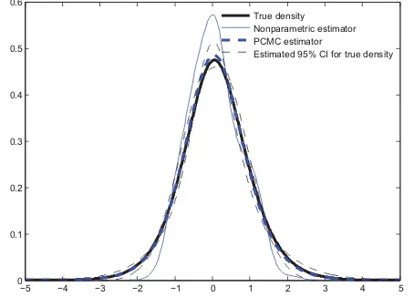
Further illustration is given inFigure 3. The figure shows the true stationary distributionf(·, θ0) in bold, one observation of ˆ
sfor the same sample size and parameters, and one observation of ˆf with the estimated 95% pointwise confidence bands for
f(·, θ0) under the same sample size and parameters. (See the discussion in Section3.2.)
−200 −15 −10 −5 0 5 10 15 20
.01 .02 .03 .04 .05 .06 .07 .08
True density Semiparametric estimator PCMC estimator
Estimated 95% CI of true density
Figure 3. Realizations of ˆsand PCMC in dynamic factor model.
4.2 Linear AR(1)
In this section, we study another simple example to further illustrate conceptual issues: the scalar Gaussian AR(1) model from (17). The construction of the PCMC density estimator for this model was discussed in Example 3.1. InFigure 2, we looked at asymptotic variance at a point. Here we look at finite sample MISE (error over the whole domain).
To study the MISE of the PCMC density estimator offin finite samples, we compare its MISE with that of the semiparametric estimator ˆs, the direct parametric alternative ˆz, the ordinary parametric alternative (OPE), and the NPKDE whenn=200. (In this case, the OPE estimates f by observing that f(y)=
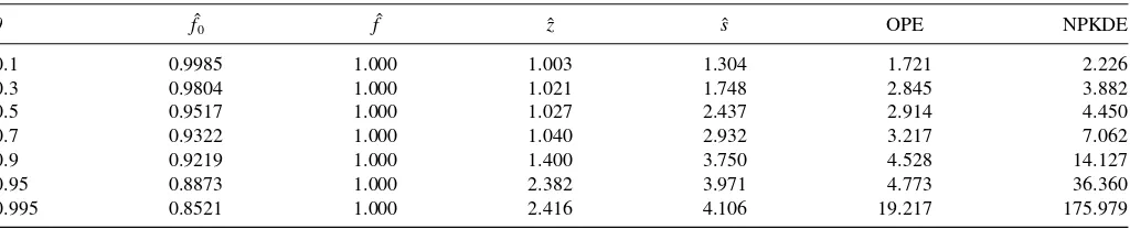
N(0,1/(1−θ2)) and estimating θ by maximum likelihood.) The method for implementing the NPKDE is identical to that used in Section 4.1. The correlation coefficient θ is the only parameter, and it is set to 0.1, 0.3, 0.5, 0.7, 0.9, 0.95, and 0.995 in seven separate experiments. We also compare ˆf0 with the PCMC density estimator to see how model estimation error influences the estimator under the AR(1) process.
Table 2presents results. All MISE values are expressed as
multiples of the MISE for the PCMC density estimator. Of the estimators that can be implemented in practice (i.e., all but ˆf0), the MISE for the PCMC density estimator is lowest for all values ofθ. Notice also that the differences become more pronounced asθincreases. This result reiterates the point made in the previ-ous section: The PCMC density estimator’s use of a parametric model for the DGP{Xt}provides the ancillary benefit of
exploit-ing the information contained in the order of the sample. When
θ =0.1, the data is almost iid, and preserving the order infor-mation in an estimate ofφhas relatively little value. The benefit becomes larger when the persistence in the DGP increases. (Ac-tually the preceding intuition best explains the improvement that
ˆ
f makes over ˆz, both of which are parametric. Another factor at
Table 2. Relative MISE values for the AR(1) model
θ fˆ0 fˆ zˆ sˆ OPE NPKDE
0.1 0.9985 1.000 1.003 1.304 1.721 2.226
0.3 0.9804 1.000 1.021 1.748 2.845 3.882
0.5 0.9517 1.000 1.027 2.437 2.914 4.450
0.7 0.9322 1.000 1.040 2.932 3.217 7.062
0.9 0.9219 1.000 1.400 3.750 4.528 14.127
0.95 0.8873 1.000 2.382 3.971 4.773 36.360
0.995 0.8521 1.000 2.416 4.106 19.217 175.979
work is that more persistent data are in essence less informative than relatively independent observations. Hence, the effective data size shrinks as we increase θ. This helps to explain why the nonparametric estimator—which has relatively weak finite sample properties—becomes less competitive.) Again, the esti-mation effect appears fairly weak when the AR(1) model is well estimated.
4.3 Threshold Autoregression
As our next application, we replace the linear AR(1) model with the nonlinear threshold autoregression (TAR) model
Yt=θ|Yt−1| +
1−θ2ξ
t, {ξt}
IID
∼ N(0,1).
The stationary density ofYthas the skew-normal formf(y)=
2ψ(y)(sy),wheres:=θ/√1−θ2, andψandare the stan-dard normal density and cumulative distribution, respectively (see Andel, Netuka, and Svara1984). The parameterθcan be estimated consistently by maximum likelihood. Following the simulations in Zhao (2010), we setθ=0.6 andn=200. The MISE for the PCMC was found to be 5.836×10⁻⁴. The MISE for ˆs was 1.945 times larger, while that for the NPKDE was 8.823 times larger.
4.4 Markov Regime Switching
Next we consider a Markov regime switching model, to il-lustrate how the PCMC estimator is implemented in a latent variable model. The model we consider here is
Yt =μXt+σXtξt, {ξt}
IID
∼N(0,1),
where {Xt} is an unobservable two-state Markov chain with
ergodic transition matrix. The stationary density ofYthas the
formf =N(μ1, σ12)×π1+N(μ2, σ22)×π2, where (π1, π2) is the stationary distribution of. The model is estimated using maximum likelihood. The PCMC density estimator can then be implemented to obtain an estimate of f. In this case, the conditional density p in (10) is p(y|X∗
t,θˆn)=N( ˆμX∗ t,σˆ
2
X∗ t).
The values {X∗
t} are simulated from a maximum likelihood
estimate ˆof the matrix.
We investigate the finite sample performance of the PCMC estimator by comparing the MISE with that of the NPKDE when
n=500. (The semiparametric estimator is not available for comparison here because the stateXt is latent.) The parameters
are set according to Smith and Layton’s (2007) business cycle analysis, withμ1=0.34,μ2 = −0.13,σ1 =0.38,σ2=0.82,
and
=
0.97 0.03 0.08 0.92
.
The MISE of the PCMC estimator was found to be 9.418×
10−3, while that of the NPKDE was 0.015. Thus, the MISE of the NPKDE was roughly 1.6 times larger.
4.5 Stochastic Volatility in Mean
As another application of the PCMC density estimator in a latent variable setting, we consider the stochastic volatility in mean model
Yt =c σ2exp(ht)+σexp(ht/2)ξt (20)
ht =κht−1+σηηt. (21)
Typically, Yt denotes return on a given asset, and the latent
variable ht denotes underlying volatility. The pair (ξt, ηt) is
standard normal inR2and iid. Parameters in the model can be estimated by simulated maximum likelihood estimate (MLE; see, e.g., Koopman and Uspensky 2002). We take ht as the
covariateXt in the definition of the PCMC density estimator,
which then has the form
ˆ
fm(y)=
1
m
m
t=1
p(y|h∗t,θˆn),
where, in view of (20), p(y|h,θˆn) :=N( ˆcnσˆn2exp(h),
ˆ
σ2
nexp(h)), and{h∗t}is generated by iterating on the estimated
version of (21).
As with the Markov switching model, we investigate the finite sample performance of the PCMC estimator by comparing its MISE with that of the NPKDE whenn=500. We adopt the estimated parameter values in Koopman and Uspensky (2002), withκ =0.97,ση=0.135,σ2=0.549, andc=1. For these
parameters, we calculated the MISE of the PCMC estimator to be 1.524×10⁻⁴, while that of the NPKDE was 3.048
×10−4. Thus, the MISE of the NPKDE was roughly 2.3 times larger. Typical realizations of the estimators and the estimated 95% confidence bands are presented inFigure 4.
5. ROBUSTNESS
Regarding the PCMC density estimator, one concern is that its advantages stem from parametric specification of the DGP of
{Xt}, and this specification may be inaccurate. In this section, we
take two models and investigate the performance of the PCMC
−5 −4 −3 −2 −1 0 1 2 3 4 5
Estimated 95% CI for true density
Figure 4. NPKDE and PCMC in the stochastic volatility in mean model.
estimator when the DGP is slightly misspecified. The first is a scalar model of the form
Yt =βXt+ξt and Xt+1=γ Xt+θ ηt+ηt+1, (22) whereβ =1,θ=0.1, and (ξt, ηt) is iid and standard normal
inR2. We vary the value ofγ from 0.4 to 0.8 to investigating the sensitivity of the estimator performance to the degree of persistence of the data. The DGP for{Xt}is misspecified as the
AR(1) process
Xt+1=γ Xt+ηt+1. (23)
Table 3reports the MISE of the PCMC density estimator
calcu-lated in the usual way, the misspecified PCMC density estimator (when the true process is (22) but the DGP of{Xt}is
misspeci-fied as (23)), the estimator ˆs, and the NPKDE (all relative to the correctly specified PCMC). While the misspecification affects the performance of the PCMC estimator, in this case the effect is relatively small.
6. PROOFS
We introduce some simplifying notation. First, letF(θ) repre-sent the functionf(·, θ) regarded as an element ofL2(X). Thus, a Markov process from such a transition density can always be
Table 3. MISE comparison, scalar factor model
γ PCMC Misspecified PCMC sˆ NPKDE
0.4 1.000 1.112 3.426 5.868
0.5 1.000 1.280 4.943 6.851
0.6 1.000 1.501 5.706 7.234
0.7 1.000 1.701 6.706 9.520
0.8 1.000 1.235 5.325 8.712
represented in the form
Xθt+1=H(Xθt, ηt+1, θ) and X0θ=x∈X, (25) whereη:= {ηt}t≥1is iid with marginalυover shock spaceDand His a suitably chosen function (see Bhattacharya and Majumdar
2007, p. 284). We letυ∞:=υ×υ× · · · be the joint law for the shocks, defined on the sequence spaceD∞.
We begin with a simple lemma regarding the function
fk′(y) := ∂f(∂θy, θ0)
k
. (26)
Lemma 6.1. Under Assumption 3.1, we have f′
k(y)=
This statement is valid if there exists an integrable functionh onXsuch that, for allθon a neighborhoodNofθ0, U and g are as defined in Assumption 3.1. By the condi-tions of Assumption 3.1, the function h is integrable, and
d(x, y, θ)E≤h(x) for allθ∈N. This implies the inequality
in (27), and Lemma 6.1 is proved.
Lemma 6.2. If Assumption 3.1 holds, thenF is Hadamard differentiable atθ0, with Hadamard derivativeFθ′0given by
Fθ′0(θ)=
operator, observe that, by the Cauchy–Schwartz inequality and Assumption 3.1,
The finiteness of the integral expression is guaranteed by Assumption 3.1. Boundedness of the operator follows.
We now turn to the verification of (29). Fixtn↓0 andθn→
θ ∈. Let
ζ(x, y, θ) :=p(y|x, θ)φ(x, θ) (y ∈Y, x∈X, θ∈)
and
Thus, (29) will be established if we can show that
n(x, y)dx
2
dy →0 (n→ ∞). (31)
As a first step, note thatn→0 pointwise onX×Y. This
first result is almost immediate from the definition of n in
(30), since, for givenxandy, the vectord(x, y, θ0) is the vector
To pass the limit through the integrals in (31), we next show that a scalar multiple of the functiong defined in Assumption 3.1 dominatesnpointwise onX×Yfor all sufficiently large
n. To see that this is the case, fix (x, y)∈X×YandN∈Nsuch thatθ0+tnθn∈Ufor alln≥N. Without loss of generality, we
can choose the neighborhoodUto be convex. With convexU, the mean value theorem in RK implies existence of a vector
θ∗
n ∈Uon the line segment betweenθ0andtnθnwith
ζ(x, y, θ0+tnθn)−ζ(x, y, θ0)= d(x, y, θn∗), tnθn.
Dividing both sides bytn and using the definition ofnin
(30), we obtain
bounded in n, and hence there exists a constant L with
|n(x, y)| ≤Lg(x, y) for alln≥N.
Returning to the proof of (31), define
hn(y) :=
everywhere on Y. To see this, observe that Assumption 3.1 gives h(y)dy <∞, and hencehis finite almost everywhere.
is so, observe that, in addition tohn→0 almost everywhere,
we have 0≤hn≤hfor alln, andhis integrable by Assumption
3.1. Another application of the dominated convergence theorem now gives hn(y)dy →0. The convergence hn(y)dy →0 is
equivalent to (31), completing the proof of Lemma 6.2.
Lemma 6.3. Under the conditions of Theorem 3.1, we have
√
n{f(·,θˆn)−f(·, θ0)} d
→N(0, C), whereN(0, C) is the cen-tered Gaussian defined in Equations (13) and (15).
Proof of Lemma 6.3.LetJbe a random variable onRK with
J ∼N(0, ), so that√n( ˆθn−θ0) converges in distribution to inL2(Y). Lemma 6.2 showed thatFis Hadamard differentiable atθ0, when viewed as a mapping fromtoL2(Y). Applying a functional delta theorem (e.g., van der Vaart1998, theorem 20.8), we obtain√n{F( ˆθn)−F(θ0)}
d
→Fθ′0(J) inL2(Y), where
Fθ′0 is as defined in (28). Thus, it remains only to show that
Fθ′0(J)∼N(0, C). Recalling the definition offk′ in (26) and using Lemma 6.1, we have
Fθ′
and the right-hand side is square-integrable by Assumption 3.1. It follows thatFθ′ This follows immediately from the fact thatJ is multivariate Gaussian, since linear combinations of multivariate Gaussian
random variables are univariate Gaussian by definition, and
element, we need to show that the (scalar) expectation of (33) is zero for allh∈L2(Y). This is true becauseEJk=0 for allm.
Finally, we need to verify that the covariance operator of
F′
Using our notation forfi′above, we can reduce this to
g, Ch =
On the other hand, regarding the left-hand side of (34), we have
Passing the expectation through the sum yields (35). In other
words, (34) is valid.
Lemma 6.4. If the conditions of Theorem 3.1 hold, then
τ(n)1/2fˆτ(n)(·,θˆn)−f(·,θˆn)
=OP(1).
Proof. The claim in Lemma 6.4 is that the term is bounded in probability overn. A sufficient condition for boundedness in probability is that the square of this term is bounded in expec-tation, which is to say that
sup
Applying Fubini’s theorem and multiplying and dividing by the square of the functionρin Assumption 3.2, we have
E
By Fatou’s lemma, we have
lim sup and hence, applying the asymptotic normality results in theorem 17.0.1 of Meyn and Tweedie (2009),
lim sup
whereγ2is a finite quantity. In consequence,
lim sup
The right-hand side is finite, sinceρ ∈L2(Y) by Assumption 3.2. The claim in (37) now follows.
Applying (37) now gives the desired result.
Proof of Theorem 3.1.Adding and subtracting f(·,θˆn), we
2002, Lemma 11.9.4). In view this fact and the result in Lemma
6.3, it suffices to show that
√
nfˆτ(n)·,θˆn−f·,θˆn=oP(1).
To see that this holds, observe that
√
nfˆτ(n)(·,θˆn)−f(·,θˆn)
=
n
τ(n)
1/2
τ(n)1/2fˆτ(n)(·,θˆn)−f(·,θˆn)
.
By Lemma 6.4 the term on the far right isOP(1). By
assump-tion we haveτ(n)/n→ ∞and hencen/τ(n)→0. The claim
follows.
ACKNOWLEDGMENTS
This article has benefited from helpful comments by Dennis Kristensen and participants at the 2012 International Sympo-sium on Econometric Theory and Applications in Shanghai, and the 18th International Conference on Computing in Economics and Finance in Prague. The authors thank Varang Wiriyawit for research assistance and ARC Discovery Outstanding Researcher Award DP120100321 for financial support.
[Received January 2014. Revised August 2014.]
REFERENCES
A¨ıt-Sahalia, Y., Fan, J., and Peng, H. (2009), “Nonparametric Transition-Based Tests for Jump Diffusions,”Journal of the American Statistical Association, 104, 1102–1116. [595]
A¨ıt-Sahalia, Y., and Hansen, L. P. (2009),Handbook of Financial Econometrics
(Vol. 1), North Holland. [595]
Andel, J., Netuka, I., and Svara, K. (1984), “On Threshold Autoregressive Processes,”Kybernetika, 20, 89–106. [602]
Bhattacharya, R. N., and Majumdar, M. (2007),Random Dynamical Systems: Theory and Applications, Cambridge: Cambridge University Press. [603] Bosq, D. (2000),Linear Processes in Function Space, New York:
Springer-Verlag. [598]
Braun, R. A., Li, H., and Stachurski, J. (2012), “Generalized Look-Ahead Methods for Computing Stationary Densities,”Mathematics of Operations Research, 37, 489–500. [596]
Calabrese, R., and Zenga, M. (2010), “Bank Loan Recovery Rates: Measuring and Nonparametric Density Estimation,”Journal of Banking and Finance, 34, 903–911. [595]
de Vincent-Humphreys, R., and Noss, J. (2012), “Estimating Probability Dis-tributions of Future Asset Prices: Empirical Transformations From Option-Implied Risk-Neutral to Real-World Density Functions,” Bank of England Working Paper No. 455. [595]
Dudley, Richard M. (2002),Real Analysis and Probability, (vol. 74), Cambridge University Press. [605]
Escanciano, J. C., and Jacho-Ch´avez, D. T. (2012), “√n-Uniformly Consis-tent Density Estimation in Nonparametric Regression Models,”Journal of Econometrics, 167, 305–316. [596]
Frees, E. W. (1994), “Estimating Densities of Functions of Observations,” Jour-nal of the American Statistical Association, 89, 517–525. [596]
Gelfand, A. E., and Smith, A. F. M. (1990), “Sampling-Based Approaches to Calculating Marginal Densities,”Journal of the American Statistical Asso-ciation, 85, 398–409. [596]
Gine, E., and Mason, D. M. (2007), “On Local U-Statistic Processes and the Estimation of Densities of Functions of Several Sample Variables,”The Annals of Statistics, 35, 1105–1145. [596]
He, L., Huh, S. W., and Lee, B. S. (2010), “Dynamic Factors and Asset Pricing,”
Journal of the American Statistical Association, 45, 707–737. [600] Henderson, S. G., and Glynn, P. W. (2001), “Computing Densities for
Markov Chains via Simulation,”Mathematics of Operations Research, 26, 375–400. [596]
Kim, K., and Wu, W. B. (2007), “Density Estimation for Nonlinear Time Series,” Mimeo, Michigan State University. [596]
Koopman, S. J., and Uspensky, E. H. (2002), “The Stochastic Volatility in Mean Model: Empirical Evidence From International Stock Markets,”Journal of Applied Econometrics, 17, 667–689. [602]
Martin, V., Hurn, S., and Harris, D. (2012),Econometric Modelling with Time Series Specification, Estimation and Testing, Cambridge: Cambridge Uni-versity Press. [595]
Meyn, S., and Tweedie, R. W. (2009),Markov Chains and Stochastic Stability
(2nd ed.), Cambridge: Cambridge University Press. [599,605]
Polanski, A., and Stoja, E. (2011), “Dynamic Density Forecasts for Multivariate Asset Returns,”Journal of Forecasting, 30, 523–540. [595]
Rosenblatt, M. (1956), “Remarks on Some Non-Parametric Estimates of a Density Function,” The Annals of Mathematical Statistics, 27, 832–837. [595]
Saavedra, Angeles and Cao, Ricardo. (2000), “On the Estimation of the Marginal Density of a Moving Average Process,”Canadian Journal of Statistics, 28(4), 799–815. [596]
Schick, A., and Wefelmeyer, W. (2004), “Functional Convergence and Opti-mality of Plug-in Estimators for Stationary Densities of Moving Average Processes,”Bernoulli, 10, 889–917. [596]
——— (2007), “Uniformly Root-n Consistent Density Estimators for Weakly Dependent Invertible Linear Processes,”The Annals of Statistics, 35, 815– 843. [596]
Smith, D. R., and Layton, A. (2007), “Comparing Probability Forecasts in Markov Regime Switching Business Cycle Models,”Journal of Business Cycle Measurement and Analysis, 479–498. [602]
Støve, B., and Tjøstheim, D. (2012), “A Convolution Estimator for the Density of Nonlinear Regression Observations,”Scandinavian Journal of Statistics, 39, 282–304. [596]
Van der Vaart, A. W. (1998),Asymptotic Statistics, Cambridge University Press. [603,604]
Zhao, Z. (2010), “Density Estimation for Nonlinear Parametric Models With Conditional Heteroskedasticity,” Journal of Econometrics, 155, 71–82. [596,597,602]
——— (2011), “Nonparametric Model Validations for Hidden Markov Models With Applications in Financial Econometrics,”Journal of Econometrics, 162, 225–239. [597]