MODELING ECONOMIC GROWTH OF DISTRICTS IN THE PROVINCE OF BALI USING SPATIAL ECONOMETRIC PANEL DATA MODEL.

(1)

M – 3

MODELING ECONOMIC GROWTH

OF DISTRICTS IN THE PROVINCE OF BALI

USING SPATIAL ECONOMETRIC PANEL DATA MODEL

Ni Ketut Tri Utami, Setiawan

Institut Teknologi Sepuluh Nopember Surabaya

Abstract

Economic growth is an important indicator to point out the success of regional development. On the framework of planning and evaluating regional development, an econometric model used to model the economic growth will be required. Since regional economic growth is often related to other regions, it is necessary to propose an econometric model that can accommodate spatial dependencies between regions. The application of spatial econometric model in modeling economic growth of districts in the Province of Bali will be constrained due to limitation on the cross sectional unit which are only nine districts. It can be overcome by using panel data, hence spatial econometric panel data models will be used to model the economic growth of districts in the Province of Bali. The kind of spatial weight used in this research is customized in order to suit the characteristics of the regions in the Province of Bali. Customized weight is formed based on the share of common side or vertex as the queen contiguity and also consider the existence Denpasar and Badung as the center of economic activities. Therefore, it can be assumed that they have a relationship with each district in the Province of Bali. The result of this research shows that the best model is Spatial Error Model (SEM) random effect and the significant variables on influencing the economic growth of districts in the Province of Bali such as: local revenue, capital expenditures, electrification ratio, mean years school and gross enrollment rate.

Key words: econometrics, economic growth, panel data, spatial

INTRODUCTION

Modeling for economic growth is needed as a reference in planning and evaluation of development. Some experts have introduced econometric model for economic growth, one of them is Robert Solow (Sardadvar, 2011) who was introduced the neoclassical model. Along with the development of closed economy to the concept of an open economy, the neoclassical Solow model of economic growth developed with the addition of technological progress factor. Mankiw, Romer, and Weil (Sardadvar, 2011) proposed to include the human resources factor (human capital) in addition to physical capital (physical capital).

(2)

correlated (Anselin, 1988).

The aim of this study is modeling the economic growth of districs in the Province of Bali. In the analysis of economic growth of the region, the indicators that show the real economic growth per capita population of a region is the GDP per capita at constant prices (Badan Pusat Statistik [BPS], 2014). Based on BPS data in 2007-2012, GDP per capita of districts in the Province of Bali recorded an increase from year to year. Hence, the factors that affect the economic growth of districts in the Province of Bali seems particularly important. This study also going to consider the existence of spatial interaction to model the economic growth of districts in the Province of Bali, hence the spatial econometric model will be used. However, the application of spatial econometric model in modeling economic growth of districts in the Province of Bali will be constrained due to limitations on the cross sectional unit which are only nine districts. Therefore, it is necessary to use panel data to accommodate the limitation of the cross section units. Panel data is a combination of cross section data and time series data where the same cross section units are measured at different times (Baltagi, 2005).

This study focuses on examine the characteristics of economic growth in Bali by considering the spatial dependencies between districts using panel data. Two spatial panel econometric models will be proposed, they are Spatial Autoregressive Model (SAR) and Spatial Error Model (SEM) with fixed effect and random effect and will be estimated using Maximum Likelihood Estimation (MLE).

RESEARCH METHOD

The secondary data of economic growth variables obtained from the Badan Pusat Statistik (BPS) of Bali from 2007 until 2012 will be used in this study. The cross section units are 9 districts in the Province of Bali.

Table 1. Research Variables

Variable Variable Name Data Scale Denomination Dependen Variable _Y GDRP per Capita Ratio Rupiah

Independen Variable X₁ Local Revenue Ratio Thousand rupiah

2

X Capital Expenditures Ratio Thousand rupiah

3

X Labour Ratio People

4

X Electrification Ratio Ratio Household

5

X Mean Years School Ratio Year

6

X Gross Enrollment Rate Ratio Persen

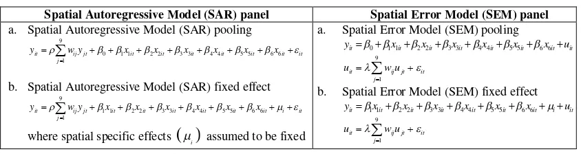
This variables were been selected based on Mankiw, Romer, and Weil model (Sardadvar, 2011), hence it will be using log-normal (ln) form. There are two spatial panel models will be built in this study, they are Spatial Autoregressive Model (SAR) and Spatial Error Model (SEM). Both spatial models will be including fixed effect and random effect panel model. The model specifications were described in Table 2.

Table 2. Model Specification

Spatial Autoregressive Model (SAR) panel Spatial Error Model (SEM) panel a. Spatial Autoregressive Model (SAR) pooling

9

b. Spatial Autoregressive Model (SAR) fixed effect

9

a. Spatial Error Model (SEM) pooling

0 1 1 2 2 3 3 4 4 5 5 6 6

b. Spatial Error Model (SEM) fixed effect

(3)

c. Spatial Autoregressive Model (SAR) random effect

c. Spatial Error Model (SEM) random effect

1 1 2 2 3 3 4 4 5 5 6 6 common side or vertex with the region of interest, and w_ij 0 for all other elements (LeSage, 1999). Customized weight is formed based on characteristics of problem of interest (Baltagi et al., 2012). In forming the customized weight, it is necessary to consider the presence of Denpasar and Badung as the center of all economic activities in the Province of Bali. Therefore, customized weight wil be formed based on the share of common side or vertex as the queen contiguity and also assumed that Denpasar and Badung have dependencies to every districts in the Province of Bali, then the weight between each districts in the Province of Bali and those

The procedure to model the economic growth in Bali using spatial econometric panel data models (SAR panel, SEM panel) described in this following steps: creating a panel regression model and calculate the parameter estimates and residual value; first testing the spatial dependencies by using lagrange multiplier test (LM) and robust lagrange multiplier for lag and error, with provisions: if the LM lag test or robust LM lag test significant, then the appropriate model is SAR panel, otherwise if the LM error test or robust LM error significant, then the appropriate model is SEM panel; modeling the panel fixed effect and random effect for both of spatial panel models; comparing the fixed effect model and random effect between each spatial panel models using Haussman specifications test; selecting the best model of each spatial panel

models by 2 2 2 , ,

R corr  criterions; comparing models obtained by using both of spatial weights (queen contiguity and customized) and selecting the best model by 2 2 2

, ,

R corr  criterions; and the last is interpretating the best model.

RESULT AND DISCUSSION

(4)

Table 3. Lagrange Multiplier (LM) Test

LM test

Queen Contiguity Customized Pooled Regression Spatial Fixed

Effect

Pooled Regression Spatial Fixed Effect

The results of lagrange multiplier test using either queen contuguity and customized indicate that spatial dependencies are occurred among districts in the Province of Bali in terms of economic growth, therefore modeling economic growth using spatial econometric panel data models will be required.

A. Queen Contiguity 1. SAR panel

Table 4. Estimation Results of Spatial Autoregressive Model (SAR) Pooling

Variable Coefficient Asymptot t-stat

P-value intercept 13.51132 10.64626 0.000000** X1 0.174235 6.188763 0.000000**

P-value intercept 11.56679 13.54937 0.000000** X1 0.17751 6.474996 0.000000** Autoregressive Model (SAR) Fixed Effect

Variable Coefficient Asymptot t-stat Autoregressive Model (SAR) Random Effect

 0.025267 3.000631 0.002694** R2 0.9969

(5)

R2 0.9962

 43.81408 2.059207 0.039474** R2 _0.9726

Corr2 0.4773

2 _0.0041

Based on Haussman specification test for SAR, where Haussman test-statistic is 19.9740 with p-value 0.0056, it could be concluded that SAR fixed effect is better to model the economic growth. Otherwise, for SEM, where Haussman test-statistic is 200.8543 with p-value 0.0000, it could be concluded that SEM fixed effect is is better to model the economic growth. By comparing SAR and SEM, SAR fixed effect has bigger R2 and corr2 and smaller 2 than SEM fixed effect, therefore the best model is Spatial Autoregressive Model (SAR) fixed effect.

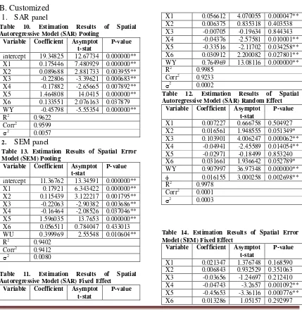
B. Customized

1. SAR panel

Table 10. Estimation Results of Spatial Autoregressive Model (SAR) Pooling

P-value intercept 19.34825 12.67734 0.000000** X1 0.175446 7.480929 0.000000**

P-value intercept 11.36762 13.34591 0.000000** X1 0.17921 6.343422 0.000000** Autoregressive Model (SAR) Fixed Effect

Variable Coefficient Asymptot t-stat Autoregressive Model (SAR) Random Effect

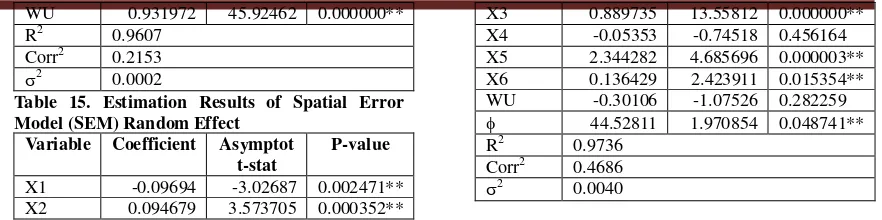
 0.016155 3.000258 0.002698** R2 0.9978

(6)

WU 0.931972 45.92462 0.000000** R2 0.9607

Corr2 0.2153

2

0.0002

Table 15. Estimation Results of Spatial Error Model (SEM) Random Effect

P-value X1 -0.09694 -3.02687 0.002471** X2 0.094679 3.573705 0.000352**

X3 0.889735 13.55812 0.000000** X4 -0.05353 -0.74518 0.456164 X5 2.344282 4.685696 0.000003** X6 0.136429 2.423911 0.015354** WU -0.30106 -1.07526 0.282259

 44.52811 1.970854 0.048741** R2 0.9736

Corr2 0.4686

2 _0.0040

Based on Haussman specification test for SAR, where Haussman test-statistic is

16.8131

with p-value

0.0186

, it could be concluded that SAR fixed effect is is better to model the economic growth. Otherwise for SEM, where Haussman test-statistic is 307.5550 with p-value 0.0000, it could be concluded that SEM fixed effect is is better to model the economic growth.

By comparing SAR and SEM

, SAR fixed effect has bigger R2 and corr2 and smaller 2 than SEM fixed effect, therefore the best model is Spatial Autoregressive Model (SAR) fixed effect.

From the best model using queen contiguity and custumized spatial weight, one of the best model will be selected using R2, corr2, and 2 criterions. Spatial Autoregressive Model

(SAR) fixed effect using customized spatial weight has bigger R2 and smaller 2 than Spatial Autoregressive Model (SAR) fixed effect using queen contiguity but smaller 2

corr , it also have more significant variables, therefore it can be concluded that the best model is Spatial Autoregressive Model (SAR) fixed effect using customized spatial weight.

Spatial Autoregressive Model (SAR) fixed effect using customized spatial weight could be written as:

9

1 2 3 4 5 6

1

0.764969 0.056612 0.006375 0.00705 0.04376 0.33516 0.030912 +

it ij jt it it it it it it it

j

y w y x x x x x x 





     

From this model, it could be shown that higher electrification ratios restrain GDRP per capita with elasticity amounts to 0.04376 and higher mean years school also restrain GDRP per capita with elasticity amounts to 0.33516. The interpretation of this model is inappropriate to economic growth model, which are all the predictors should give a positive effects to output of economic growth, in this case GDRP per capita. It could be happen due to multicollinearity among predictors. To detect multicollinearity, one may calculate the Variance Inflation Factor (VIF) and correlation among predictors.

Table 16. Variance Inflation Factors (VIF)

Variable VIF

X1 7.522

X2 2.667

X3 7.905

X4 12.914

X5 3.142

X6 1.798

Table 17. Pearson’s Correlation among Predictors

Variable Y X1 X2 X3 X4 X5

X1 0.786

0.000**

X2 0.509 0.660

0.000** 0.000**

X3 0.280 0.676 0.299

(7)

Table 16 shows Variance Inflation Factor (VIF) of X4 is more than 10, it indicate that multicollinearity was occurred. From the correlation among predictors on Table 17, it could be shown there are positive correlation between predictors. This multicollinearity problem causes inconsistency in parameter estimation, as a result the coefficient of parameters have a wrong sign. To overcome this problem, the predictors that may cause multicollinearity will not be included to model. One way to select those predictors is considering the predictor that have a bigger correlation to other predictors than to response, in this case are X1, X2, X3 and X4. Therefore, those predictors will be deleted from model one by one and also considering its combination. Tables below show the best model using each spatial weights.

Table 18. Estimation Results of Spatial Error Model (SEM) Random Effect (without Labour and Electrification Ratio) using Queen Contiguity Spatial Weight

Variable Coefficient Asymptot t-stat

z-probability X1 0.366654 5.498841 0.000000** X2 0.190752 5.250846 0.000000** X5 2.211259 3.901859 0.000095** X6 0.210023 2.664311 0.007715** WU 0.805171 13.85293 0.000000**

 23.66447 2.126499 0.033462** R2 _0.9365

Corr2 0.8068

2 _0.0096

Table 19. Estimation Results of Spatial Error Model (SEM) Random Effect (without Labour) using Customized Spatial Weight

Variable Coefficient Asymptot t-stat

z-probability X1 0.346365 5.301239 0.000000** X2 0.158785 4.002521 0.000063** X4 0.156773 1.929859 0.053624* X5 1.966090 3.340348 0.000837** X6 0.157756 2.194700 0.028185** WY 0.830123 15.780649 0.000000**

 28.233915 2.057099 0.039677** R2 0.9478

Corr2 0.7761

2

0.0079

The best model will be selected using 2 2 2 , , and

R corr 

_criterions.

Spatial Error Model (SEM) random effect using customized spatial weight has bigger R2 and smaller 2

than

Spatial Error Model (SEM) random effect using queen contiguity but smaller corr2, it also have more significant variables, therefore it can be concluded that the best model is Spatial Error Model (SEM) random effect using customized spatial weight.

Spatial Error Model (SEM) random effect using customized spatial weight could be written as:

1 2 4 5 6

9

1

0.346365 0.158785 +0.156773 1.966090 0.157756 0.830123

it it it it it it it

it ij jt it j

y x x x x x u

u w u 



    







From this model, it could be shown that higher local revenues have a positive significant effects to GDRP per capita with elasticity amounts to 0.346365. Higher capital expenditures have a positive significant effects to GDRP per capita with elasticity amounts to 0.158785. Higher electrification ratios have a positive significant effects to GDRP per capita with elasticity amounts to 0.156773. Higher mean years school have a positive significant effects to GDRP per capita with elasticity amounts to 0.966090. And the last, higher gross enrollment rates have a positive significant effects to GDRP per capita with elasticity amounts to 0.157756. The spatial error model shows that error of the model of one region and the neighboring regions is spatially correlated.

CONCLUSION AND SUGGESTION

(8)

multicollinearity problem was occurred. It causes inconsistency in parameter estimation, as a result the coefficient of parameters have a wrong sign. To overcome this problem, the predictors that may cause multicollinearity were deleted from the model. The best model is selected using

2 2 2

, , and

R corr 

_criterions.

Spatial Error Model (SEM) random effect using customized spatial weight is the best model and the significant variables on influencing the economic growth of districts in the Province of Bali are local revenue, capital expenditures, electrification ratio, mean years school and gross enrollment rate.

REFERENCES

Anselin, L. (1988), Spatial Econometrics: Methods and Models, Kluwer Academic Publishers, The Netherlands.

Badan Perencanaan Pembangunan Nasional (2012), Pembangunan Daerah dalam Angka 2012, Bappenas, Jakarta.

Badan Pusat Statistik (2014), Sistem Rujukan Statistik, BPS, Jakarta. http://sirusa.bps.go.id/

Baltagi, B.H. (2005), Econometrics Analysis of Panel Data, 3rd edition, John Wiley & Sons Ltd, England.

Baltagi, B.H., Blien, U. & Wolf, K. (2012), “A Dynamic Spatial Panel Data Approach to The German Wage Curve”, Economic Modelling, Elsevier, Vol. 29(1), hal. 12-21.

Elhorst, J.P. (2014), Spatial Econometrics: From Cross-Sectional Data to Spatial Panels, Springer, Heidelberg, New York, Dordrecht, London.

LeSage, J.P. (1999), Spatial Econometrics, www.spatial-econometrics.com/html/wbook.pdf