Chapter 2
MATRICES
2.1
Matrix arithmetic
A matrix over a fieldF is a rectangular array of elements fromF. The sym-bolMm×n(F) denotes the collection of allm×nmatrices overF. Matrices will usually be denoted by capital letters and the equationA= [aij] means that the element in the i–th row and j–th column of the matrix A equals
aij. It is also occasionally convenient to write aij = (A)ij. For the present, all matrices will have rational entries, unless otherwise stated.
EXAMPLE 2.1.1 The formula aij = 1/(i+j) for 1≤ i ≤3,1 ≤j ≤ 4 defines a 3×4 matrix A= [aij], namely
A=
1
2 13 14 15
1
3 14 15 16
1
4 15 16 17
.
DEFINITION 2.1.1 (Equality of matrices) MatricesA, B are said to be equal if A and B have the same size and corresponding elements are equal; i.e., Aand B ∈Mm×n(F) and A= [aij], B = [bij], with aij =bij for 1≤i≤m, 1≤j≤n.
DEFINITION 2.1.2 (Addition of matrices) Let A = [aij] and B = [bij] be of the same size. Then A+B is the matrix obtained by adding corresponding elements ofA and B; that is
24 CHAPTER 2. MATRICES
DEFINITION 2.1.3 (Scalar multiple of a matrix) LetA= [aij] and
t∈F (that istis ascalar). Then tA is the matrix obtained by multiplying all elements ofA byt; that is
tA=t[aij] = [taij].
DEFINITION 2.1.4 (Additive inverse of a matrix) Let A = [aij] . Then −A is the matrix obtained by replacing the elements of A by their additive inverses; that is
−A=−[aij] = [−aij].
DEFINITION 2.1.5 (Subtraction of matrices) Matrix subtraction is defined for two matrices A = [aij] and B = [bij] of the same size, in the usual way; that is
A−B = [aij]−[bij] = [aij−bij].
DEFINITION 2.1.6 (The zero matrix) For each m, n the matrix in
Mm×n(F), all of whose elements are zero, is called the zeromatrix (of size
m×n) and is denoted by the symbol 0.
The matrix operations of addition, scalar multiplication, additive inverse and subtraction satisfy the usual laws of arithmetic. (In what follows,sand
twill be arbitrary scalars and A, B, C are matrices of the same size.) 1. (A+B) +C=A+ (B+C);
2. A+B =B+A; 3. 0 +A=A; 4. A+ (−A) = 0;
5. (s+t)A=sA+tA, (s−t)A=sA−tA; 6. t(A+B) =tA+tB, t(A−B) =tA−tB; 7. s(tA) = (st)A;
8. 1A=A, 0A= 0, (−1)A=−A; 9. tA= 0⇒t= 0 orA= 0.
2.1. MATRIX ARITHMETIC 25
Matrix multiplication obeys many of the familiar laws of arithmetic apart from the commutative law.
1. (AB)C=A(BC) if A, B, C arem×n, n×p, p×q, respectively; 2. t(AB) = (tA)B=A(tB), A(−B) = (−A)B =−(AB);
3. (A+B)C=AC+BC ifA and B arem×nand C isn×p; 4. D(A+B) =DA+DB ifAand B arem×nand Dis p×m.
We prove the associative law only:
26 CHAPTER 2. MATRICES
However the double summations are equal. For sums of the form n
represent the sum of thenpelements of the rectangular array [djk], by rows and by columns, respectively. Consequently
((AB)C)il= (A(BC))il for 1≤i≤m, 1≤l≤q. Hence (AB)C =A(BC).
The system of m linear equations inn unknowns
a11x1+a12x2+· · ·+a1nxn = b1
a21x1+a22x2+· · ·+a2nxn = b2
.. .
am1x1+am2x2+· · ·+amnxn = bm is equivalent to a single matrix equation
is the vector of unknowns and B =
is the vector of
constants.
2.2. LINEAR TRANSFORMATIONS 27 EXAMPLE 2.1.3 The system
x+y+z = 1
x−y+z = 0.
is equivalent to the matrix equation
·
1 1 1
1 −1 1
¸
x y z
= ·
1 0
¸
and to the equation
x ·
1 1
¸
+y ·
1 −1
¸
+z ·
1 1
¸
=
·
1 0
¸ .
2.2
Linear transformations
An n–dimensional column vectoris an n×1 matrix overF. The collection of alln–dimensional column vectors is denoted byFn.
Every matrix is associated with an important type of function called a linear transformation.
DEFINITION 2.2.1 (Linear transformation) We can associate with
A∈Mm×n(F), the functionTA:Fn→Fm, defined byTA(X) =AX for all
X ∈ Fn. More explicitly, using components, the above function takes the form
y1 = a11x1+a12x2+· · ·+a1nxn
y2 = a21x1+a22x2+· · ·+a2nxn ..
.
ym = am1x1+am2x2+· · ·+amnxn,
wherey1, y2,· · ·, ym are the components of the column vector TA(X). The function just defined has the property that
TA(sX+tY) =sTA(X) +tTA(Y) (2.1) for all s, t∈F and all n–dimensional column vectorsX, Y. For
28 CHAPTER 2. MATRICES
REMARK 2.2.1 It is easy to prove that if T : Fn → Fm is a function satisfying equation 2.1, then T = TA, where A is the m×n matrix whose columns are T(E1), . . . , T(En), respectively, where E1, . . . , En are the n– dimensionalunit vectors defined by
E1 =
1 0 .. . 0
, . . . , En=
0 0 .. . 1
.
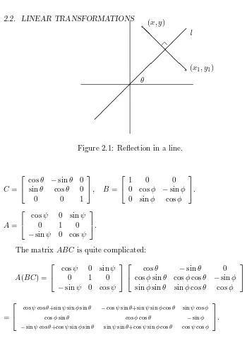
One well–known example of a linear transformation arises from rotating the (x, y)–plane in 2-dimensional Euclidean space, anticlockwise through θ
radians. Here a point (x, y) will be transformed into the point (x1, y1),
where
x1 = xcosθ−ysinθ y1 = xsinθ+ycosθ.
In 3–dimensional Euclidean space, the equations
x1 =xcosθ−ysinθ, y1 =xsinθ+ycosθ, z1 =z; x1 =x, y1 =ycosφ−zsinφ, z1=ysinφ+zcosφ; x1 =xcosψ+zsinψ, y1=y, z1=−xsinψ+zcosψ;
correspond to rotations about the positive z, x and y axes, anticlockwise through θ, φ, ψradians, respectively.
The product of two matrices is related to the product of the correspond-ing linear transformations:
IfAism×nandB isn×p, then the functionTATB :Fp→Fm, obtained by first performingTB, thenTAis in fact equal to the linear transformation
TAB. For ifX∈Fp, we have
TATB(X) =A(BX) = (AB)X=TAB(X).
The following example is useful for producing rotations in 3–dimensional animated design. (See [27, pages 97–112].)
2.2. LINEAR TRANSFORMATIONS 29
θ
l (x, y)
(x1, y1)
¡¡ ¡¡
¡¡ ¡¡
¡ ¡ ¡ ¡ ¡
❅ ❅ ❅ ❅
❅ ❅
❅
Figure 2.1: Reflection in a line.
C=
cosθ −sinθ 0 sinθ cosθ 0
0 0 1
, B =
1 0 0
0 cosφ −sinφ
0 sinφ cosφ
.
A=
cosψ 0 sinψ
0 1 0
−sinψ 0 cosψ
.
The matrix ABC is quite complicated:
A(BC) =
cosψ 0 sinψ
0 1 0
−sinψ 0 cosψ
cosθ −sinθ 0 cosφsinθ cosφcosθ −sinφ
sinφsinθ sinφcosθ cosφ
=
cosψcosθ+sinψsinφsinθ −cosψsinθ+sinψsinφcosθ sinψcosφ
cosφsinθ cosφcosθ −sinφ −sinψcosθ+cosψsinφsinθ sinψsinθ+cosψsinφcosθ cosψcosφ
.
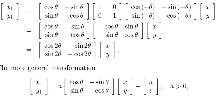
EXAMPLE 2.2.2 Another example from geometry is reflection of the plane in a linel inclined at an angleθ to the positivex–axis.
We reduce the problem to the simpler case θ = 0, where the equations of transformation are x1 = x, y1 = −y. First rotate the plane clockwise
30 CHAPTER 2. MATRICES
Figure 2.2: Projection on a line.
In terms of matrices, we get transformation equations
·
The more general transformation
·
represents a rotation, followed by a scaling and then by a translation. Such transformations are important in computer graphics. See [23, 24].
EXAMPLE 2.2.3 Our last example of a geometrical linear transformation arises from projecting the plane onto a line l through the origin, inclined at angle θ to the positive x–axis. Again we reduce that problem to the simpler case where l is the x–axis and the equations of transformation are
x1 =x, y1 = 0.
In terms of matrices, we get transformation equations
2.3. RECURRENCE RELATIONS 31
=
·
cosθ 0 sinθ 0
¸ ·
cosθ sinθ
−sinθ cosθ ¸ ·
x y
¸
=
·
cos2θ cosθsinθ
sinθcosθ sin2θ ¸ ·
x y
¸ .
2.3
Recurrence relations
DEFINITION 2.3.1 (The identity matrix) The n× n matrix In = [δij], defined by δij = 1 ifi=j, δij = 0 if i6=j, is called the n×n identity matrix of order n. In other words, the columns of the identity matrix of order nare the unit vectorsE1,· · ·, En, respectively.
For example,I2 = ·
1 0 0 1
¸
.
THEOREM 2.3.1 IfA ism×n, then ImA=A=AIn.
DEFINITION 2.3.2 (k–th power of a matrix) IfAis ann×nmatrix, we defineAk recursively as follows: A0=I
n andAk+1=AkA fork≥0. For exampleA1 =A0A=InA=Aand hence A2 =A1A=AA.
The usual index laws hold providedAB=BA: 1. AmAn=Am+n, (Am)n=Amn;
2. (AB)n=AnBn; 3. AmBn=BnAm;
4. (A+B)2 =A2+ 2AB+B2;
5. (A+B)n= n
X
i=0 ¡n
i
¢
AiBn−i;
6. (A+B)(A−B) =A2−B2.
We now state a basic property of the natural numbers.
AXIOM 2.3.1 (MATHEMATICAL INDUCTION) If Pn denotes a mathematical statement for each n≥1, satisfying
32 CHAPTER 2. MATRICES
(ii) the truth of Pn implies that ofPn+1 for each n≥1,
thenPn is true for alln≥1.
EXAMPLE 2.3.1 LetA=
·
7 4
−9 −5
¸
.Prove that
An=
·
1 + 6n 4n
−9n 1−6n ¸
if n≥1.
Solution. We use the principle of mathematical induction. Take Pn to be the statement
An=
·
1 + 6n 4n
−9n 1−6n ¸
.
ThenP1 asserts that A1 =
·
1 + 6×1 4×1 −9×1 1−6×1
¸
=
·
7 4
−9 −5
¸ ,
which is true. Now letn≥1 and assume thatPnis true. We have to deduce that
An+1=
·
1 + 6(n+ 1) 4(n+ 1) −9(n+ 1) 1−6(n+ 1)
¸
=
·
7 + 6n 4n+ 4 −9n−9 −5−6n
¸ .
Now
An+1 = AnA
=
·
1 + 6n 4n
−9n 1−6n ¸ ·
7 4
−9 −5
¸
=
·
(1 + 6n)7 + (4n)(−9) (1 + 6n)4 + (4n)(−5) (−9n)7 + (1−6n)(−9) (−9n)4 + (1−6n)(−5)
¸
=
·
7 + 6n 4n+ 4 −9n−9 −5−6n
¸ ,
and “the induction goes through”.
2.4. PROBLEMS 33 EXAMPLE 2.3.2 The following system of recurrence relations holds for alln≥0:
xn+1 = 7xn+ 4yn
yn+1 = −9xn−5yn. Solve the system forxn and yn in terms ofx0 and y0.
Solution. Combine the above equations into a single matrix equation
· xn+1 yn+1
¸
=
·
7 4
−9 −5
¸ · xn
yn
¸ ,
orXn+1 =AXn, whereA=
·
7 4
−9 −5
¸
and Xn=
· xn
yn
¸
. We see that
X1 = AX0
X2 = AX1=A(AX0) =A2X0
.. .
Xn = AnX0.
(The truth of the equation Xn = AnX0 for n ≥ 1, strictly speaking
follows by mathematical induction; however for simple cases such as the above, it is customary to omit the strict proof and supply instead a few lines of motivation for the inductive statement.)
Hence the previous example gives
· xn
yn
¸
=Xn =
·
1 + 6n 4n
−9n 1−6n ¸ ·
x0 y0
¸
=
·
(1 + 6n)x0+ (4n)y0
(−9n)x0+ (1−6n)y0 ¸
,
and hencexn= (1 + 6n)x0+ 4ny0andyn= (−9n)x0+ (1−6n)y0, forn≥1.
2.4
PROBLEMS
1. LetA, B, C, D be matrices defined by
A=
3 0 −1 2 1 1
, B =
1 5 2 −1 1 0 −4 1 3
34 CHAPTER 2. MATRICES
Which of the following matrices are defined? Compute those matrices which are defined.
A+B, A+C, AB, BA, CD, DC, D2.
for suitable numbers a and b. Use the associative law to show that (BA)2B =B.
2 and mathematical
induction, to prove that
2.4. PROBLEMS 35
whereA =
· a b
1 0
¸
and hence express
· xn+1
xn
¸
in terms of
· x1 x0
¸
. If a= 4 and b =−3, use the previous question to find a formula for
xn in terms ofx1 and x0.
[Answer:
xn=
3n−1 2 x1+
3−3n 2 x0.] 6. LetA=
·
2a −a2
1 0
¸
. (a) Prove that
An=
·
(n+ 1)an −nan+1 nan−1 (1−n)an
¸
ifn≥1.
(b) A sequencex0, x1, . . . , xn, . . . satisfies xn+1 = 2axn−a2xn−1 for n ≥ 1. Use part (a) and the previous question to prove that
xn=nan−1x1+ (1−n)anx0 forn≥1.
7. Let A =
· a b
c d ¸
and suppose that λ1 and λ2 are the roots of the
quadratic polynomialx2−(a+d)x+ad−bc. (λ1andλ2 may be equal.)
Letknbe defined by k0 = 0, k1 = 1 and forn≥2
kn= n
X
i=1
λn−i1 λi−2 1.
Prove that
kn+1= (λ1+λ2)kn−λ1λ2kn−1,
ifn≥1. Also prove that
kn=
½
(λn1 −λn2)/(λ1−λ2) ifλ16=λ2, nλn−1 1 ifλ1=λ2.
Use mathematical induction to prove that ifn≥1,
An=knA−λ1λ2kn−1I2,
36 CHAPTER 2. MATRICES
8. Use Question 7 to prove that if A=
·
1 2 2 1
¸
, then
An= 3 n 2
·
1 1 1 1
¸
+(−1) n−1
2
·
−1 1 1 −1
¸
ifn≥1.
9. The Fibonacci numbers are defined by the equations F0 = 0, F1 = 1
andFn+1=Fn+Fn−1 ifn≥1. Prove that
Fn= √1 5
ÃÃ
1 +√5 2
!n
−
Ã
1−√5 2
!n!
ifn≥0.
10. Let r > 1 be an integer. Let a and b be arbitrary positive integers. Sequencesxnand ynof positive integers are defined in terms of aand
bby the recurrence relations
xn+1 = xn+ryn
yn+1 = xn+yn, forn≥0, where x0 =aand y0 =b.
Use Question 7 to prove that
xn
yn → √
r asn→ ∞.
2.5
Non–singular matrices
DEFINITION 2.5.1 (Non–singular matrix) A matrix A ∈ Mn×n(F) is called non–singular or invertible if there exists a matrix B ∈ Mn×n(F) such that
AB=In=BA.
Any matrixB with the above property is called an inverse ofA. IfA does not have an inverse,A is called singular.
2.5. NON–SINGULAR MATRICES 37 Proof. Let B and C be inverses of A. Then AB = In = BA and AC =
In=CA. ThenB(AC) =BIn=B and (BA)C=InC=C. Hence because
B(AC) = (BA)C, we deduce thatB =C.
REMARK 2.5.1 If Ahas an inverse, it is denoted byA−1. So AA−1=In=A−1A.
Also if Ais non–singular, it follows thatA−1 is also non–singular and
(A−1)−1=A.
THEOREM 2.5.2 IfAand B are non–singular matrices of the same size, then so is AB. Moreover
(AB)−1 =B−1A−1.
Proof.
(AB)(B−1A−1) =A(BB−1)A−1 =AInA−1 =AA−1=In. Similarly
(B−1A−1)(AB) =In.
REMARK 2.5.2 The above result generalizes to a product of m non– singular matrices: IfA1, . . . , Am are non–singularn×n matrices, then the productA1. . . Am is also non–singular. Moreover
(A1. . . Am)−1 =A−m1. . . A−11.
(Thus the inverse of the product equals the product of the inverses in the reverse order.)
EXAMPLE 2.5.1 If A and B are n×n matrices satisfying A2 = B2 =
(AB)2 =In, prove thatAB=BA.
Solution. Assume A2 = B2 = (AB)2 = In. Then A, B, AB are non– singular and A−1=A, B−1 =B,(AB)−1 =AB.
But (AB)−1=B−1A−1 and henceAB=BA.
EXAMPLE 2.5.2 A =
·
1 2 4 8
¸
is singular. For suppose B =
· a b c d
¸
is an inverse ofA. Then the equation AB=I2 gives ·
1 2 4 8
¸ · a b c d
¸
=
·
1 0 0 1
38 CHAPTER 2. MATRICES
and equating the corresponding elements of column 1 of both sides gives the system
a+ 2c = 1 4a+ 8c = 0 which is clearly inconsistent.
THEOREM 2.5.3 Let A =
· a b c d
¸
and ∆ = ad−bc 6= 0. Then A is non–singular. Also
A−1= ∆−1 ·
d −b
−c a ¸
.
REMARK 2.5.3 The expression ad−bc is called the determinant of A
and is denoted by the symbols detAor
¯ ¯ ¯ ¯
a b c d
¯ ¯ ¯ ¯
.
Proof. Verify that the matrix B = ∆−1 ·
d −b
−c a ¸
satisfies the equation
AB=I2 =BA.
EXAMPLE 2.5.3 Let
A=
0 1 0 0 0 1 5 0 0
.
Verify thatA3= 5I
3, deduce thatA is non–singular and findA−1.
Solution. After verifying thatA3 = 5I3, we notice that A
µ
1 5A
2 
=I3= µ
1 5A
2 
A.
HenceA is non–singular and A−1 = 1 5A2.
THEOREM 2.5.4 If the coefficient matrix A of a system of n equations in n unknowns is non–singular, then the system AX = B has the unique solution X=A−1B.
2.5. NON–SINGULAR MATRICES 39 1. (Uniqueness.) Assume thatAX =B. Then
(A−1A)X = A−1B, InX = A−1B,
X = A−1B.
2. (Existence.) Let X=A−1B. Then
AX = A(A−1B) = (AA−1)B =InB =B.
THEOREM 2.5.5 (Cramer’s rule for 2 equations in 2 unknowns) The system
and we know that the system
A
has the unique solution
40 CHAPTER 2. MATRICES
COROLLARY 2.5.1 The homogeneous system
ax+by = 0
cx+dy = 0
has only the trivial solution if ∆ =
¯ ¯ ¯ ¯
a b c d
¯ ¯ ¯ ¯6
= 0.
EXAMPLE 2.5.4 The system
7x+ 8y = 100 2x−9y = 10
has the unique solutionx= ∆1/∆, y= ∆2/∆, where
∆=
˛ ˛ ˛ ˛ ˛ ˛
7 8
2 −9
˛ ˛ ˛ ˛ ˛ ˛
=−79, ∆1=
˛ ˛ ˛ ˛ ˛ ˛
100 8 10 −9
˛ ˛ ˛ ˛ ˛ ˛
=−980, ∆2=
˛ ˛ ˛ ˛ ˛ ˛
7 100 2 10
˛ ˛ ˛ ˛ ˛ ˛
=−130.
Sox= 98079 and y= 13079.
THEOREM 2.5.6 Let A be a square matrix. If A is non–singular, the homogeneous system AX = 0 has only the trivial solution. Equivalently, if the homogenous system AX = 0 has a non–trivial solution, then A is singular.
Proof. If Ais non–singular and AX = 0, then X=A−10 = 0.
REMARK 2.5.4 IfA∗1, . . . , A∗n denote the columns ofA, then the equa-tion
AX =x1A∗1+. . .+xnA∗n
holds. Consequently theorem 2.5.6 tells us that if there existx1, . . . , xn,not all zero, such that
x1A∗1+. . .+xnA∗n= 0,
2.5. NON–SINGULAR MATRICES 41 EXAMPLE 2.5.5
A=
1 2 3 1 0 1 3 4 7
is singular. For it can be verified thatA has reduced row–echelon form
1 0 1 0 1 1 0 0 0
and consequentlyAX = 0 has a non–trivial solutionx=−1, y=−1, z= 1. REMARK 2.5.5 More generally, if A is row–equivalent to a matrix con-taining a zero row, then A is singular. For then the homogeneous system
AX= 0 has a non–trivial solution.
An important class of non–singular matrices is that of the elementary row matrices.
DEFINITION 2.5.2 (Elementary row matrices) To each of the three types of elementary row operation, there corresponds an elementary row matrix, denoted by Eij, Ei(t), Eij(t):
1. Eij,(i6=j) is obtained from the identity matrixIn by interchanging rows iandj.
2. Ei(t),(t6= 0) is obtained by multiplying thei–th row ofIn by t. 3. Eij(t),(i=6 j) is obtained from In by adding ttimes the j–th row of
In to thei–th row. EXAMPLE 2.5.6 (n= 3.)
E23=
1 0 0 0 0 1 0 1 0
, E2(−1) =
1 0 0
0 −1 0
0 0 1
, E23(−1) =
1 0 0
0 1 −1
0 0 1
.
42 CHAPTER 2. MATRICES
COROLLARY 2.5.2 Elementary row–matrices are non–singular. Indeed 1. E−1
ij =Eij; 2. Ei−1(t) =Ei(t−1);
3. (Eij(t))−1 =Eij(−t).
2.5. NON–SINGULAR MATRICES 43 REMARK 2.5.6 Recall thatAandB are row–equivalent ifB is obtained from A by a sequence of elementary row operations. If E1, . . . , Er are the respective corresponding elementary row matrices, then
B =Er(. . .(E2(E1A)). . .) = (Er. . . E1)A=P A,
where P = Er. . . E1 is non–singular. Conversely if B = P A, where P is
non–singular, thenA is row–equivalent to B. For as we shall now see, P is in fact a product of elementary row matrices.
THEOREM 2.5.8 LetA be non–singularn×nmatrix. Then (i) Ais row–equivalent to In,
(ii) Ais a product of elementary row matrices.
Proof. Assume thatAis non–singular and letBbe the reduced row–echelon form of A. Then B has no zero rows, for otherwise the equation AX = 0 would have a non–trivial solution. ConsequentlyB =In.
It follows that there exist elementary row matricesE1, . . . , Er such that
Er(. . .(E1A). . .) = B = In and hence A = E1−1. . . Er−1, a product of elementary row matrices.
THEOREM 2.5.9 LetA be n×nand suppose that A is row–equivalent to In. Then A is non–singular and A−1 can be found by performing the same sequence of elementary row operations onIn as were used to convert
AtoIn.
Proof. Suppose that Er. . . E1A = In. In other words BA = In, where
B = Er. . . E1 is non–singular. Then B−1(BA) =B−1In and so A =B−1, which is non–singular.
Also A−1 =¡
B−1¢−1
=B =Er((. . .(E1In). . .), which shows that A−1 is obtained from In by performing the same sequence of elementary row operations as were used to convertA toIn.
REMARK 2.5.7 It follows from theorem 2.5.9 that if A is singular, then
Ais row–equivalent to a matrix whose last row is zero.
EXAMPLE 2.5.9 Show thatA=
·
1 2 1 1
¸
is non–singular, findA−1 and
44 CHAPTER 2. MATRICES
Solution. We form thepartitionedmatrix [A|I2] which consists ofAfollowed byI2. Then any sequence of elementary row operations which reduces Ato I2 will reduce I2 toA−1. Here
[A|I2] =
·
1 2 1 0
1 1 0 1
¸
R2 →R2−R1 ·
1 2 1 0
0 −1 −1 1
¸
R2 →(−1)R2 ·
1 2 1 0
0 1 1 −1
¸
R1 →R1−2R2 ·
1 0 −1 2
0 1 1 −1
¸ .
Hence A is row–equivalent toI2 andA is non–singular. Also A−1 =
·
−1 2 1 −1
¸ .
We also observe that
E12(−2)E2(−1)E21(−1)A=I2.
Hence
A−1 = E
12(−2)E2(−1)E21(−1) A = E21(1)E2(−1)E12(2).
The next result is the converse of Theorem 2.5.6 and is useful for proving the non–singularity of certain types of matrices.
THEOREM 2.5.10 Let A be an n×n matrix with the property that the homogeneous system AX = 0 has only the trivial solution. Then A is non–singular. Equivalently, if A is singular, then the homogeneous system
AX= 0 has a non–trivial solution.
Proof. If A is n×n and the homogeneous system AX = 0 has only the trivial solution, then it follows that the reduced row–echelon form B of A
2.5. NON–SINGULAR MATRICES 45 Proof. Let AB = In, where A and B are n×n. We first show that B
is non–singular. Assume BX = 0. Then A(BX) = A0 = 0, so (AB)X = 0, InX= 0 and henceX = 0.
Then fromAB=In we deduce (AB)B−1=InB−1 and henceA=B−1. The equationBB−1=I
n then givesBA=In.
Before we give the next example of the above criterion for non-singularity, we introduce an important matrix operation.
DEFINITION 2.5.3 (The transpose of a matrix) LetA be anm×n
matrix. ThenAt, thetransposeofA, is the matrix obtained by interchanging the rows and columns ofA. In other words if A = [aij], then ¡At¢ji =aij. ConsequentlyAt is n×m.
The transpose operation has the following properties: 1. ¡
At¢t
=A;
2. (A±B)t=At±Bt ifAand B arem×n; 3. (sA)t=sAt ifsis a scalar;
4. (AB)t=BtAt ifAis m×nand B isn×p;
5. IfA is non–singular, then At is also non–singular and
¡ At¢−1
=¡ A−1¢t
; 6. XtX=x2
1+. . .+x2n ifX = [x1, . . . , xn]tis a column vector.
We prove only the fourth property. First check that both (AB)t and BtAt
have the same size (p ×m). Moreover, corresponding elements of both matrices are equal. For if A= [aij] and B= [bjk], we have
¡
(AB)t¢
ki = (AB)ik =
n
X
j=1 aijbjk
= n
X
j=1 ¡
Bt¢
kj
¡ At¢
ji
= ¡ BtAt¢
ki.
46 CHAPTER 2. MATRICES
DEFINITION 2.5.4 (Symmetric matrix) A matrix A is symmetric if
At = A. In other words A is square (n×n say) and aji = aij for all 1≤i≤n, 1≤j≤n. Hence
A=
· a b
b c ¸
is a general 2×2 symmetric matrix.
DEFINITION 2.5.5 (Skew–symmetric matrix) A matrix A is called skew–symmetric if At = −A. In other words A is square (n×n say) and
aji =−aij for all 1≤i≤n, 1≤j≤n.
REMARK 2.5.8 Takingi=jin the definition of skew–symmetric matrix givesaii=−aii and so aii= 0. Hence
A=
·
0 b
−b 0
¸
is a general 2×2 skew–symmetric matrix.
We can now state a second application of the above criterion for non– singularity.
COROLLARY 2.5.4 Let B be an n×n skew–symmetric matrix. Then
A=In−B is non–singular.
Proof. Let A=In−B, where Bt=−B. By Theorem 2.5.10 it suffices to show thatAX= 0 implies X= 0.
We have (In−B)X= 0, so X=BX. Hence XtX=XtBX. Taking transposes of both sides gives
(XtBX)t = (XtX)t
XtBt(Xt)t = Xt(Xt)t
Xt(−B)X = XtX
−XtBX = XtX =XtBX.
HenceXtX=−XtX and XtX= 0. But if X= [x1, . . . , xn]t, thenXtX =
x2
2.6. LEAST SQUARES SOLUTION OF EQUATIONS 47
2.6
Least squares solution of equations
Suppose AX = B represents a system of linear equations with real coeffi-cients which may be inconsistent, because of the possibility of experimental errors in determiningA orB. For example, the system
x = 1
y = 2
x+y = 3.001 is inconsistent.
It can be proved that the associated system AtAX = AtB is always consistent and that any solution of this system minimizes the sumr12+. . .+
rm2, wherer1, . . . , rm (the residuals) are defined by
ri =ai1x1+. . .+ainxn−bi,
fori= 1, . . . , m. The equations represented byAtAX=AtB are called the normal equations corresponding to the system AX = B and any solution of the system of normal equations is called a least squares solution of the original system.
EXAMPLE 2.6.1 Find a least squares solution of the above inconsistent system.
Solution. HereA=
1 0 0 1 1 1
, X= ·
x y
¸ , B =
1 2 3.001
.
ThenAtA=
·
1 0 1 0 1 1
¸
1 0 0 1 1 1
= ·
2 1 1 2
¸
.
Also AtB =
·
1 0 1 0 1 1
¸
1 2 3.001
= ·
4.001 5.001
¸
. So the normal equations are
2x+y = 4.001
x+ 2y = 5.001 which have the unique solution
x= 3.001
3 , y= 6.001
48 CHAPTER 2. MATRICES
EXAMPLE 2.6.2 Points (x1, y1), . . . ,(xn, yn) are experimentally deter-mined and should lie on a liney=mx+c. Find a least squares solution to the problem.
Solution. The points have to satisfy
mx1+c = y1
It is not difficult to prove that
∆ = det (AtA) = X
1≤i<j≤n
(xi−xj)2,
which is positive unless x1 = . . . = xn. Hence if not all of x1, . . . , xn are equal,AtAis non–singular and the normal equations have a unique solution. This can be shown to be
m= 1
2.7. PROBLEMS 49
2.7
PROBLEMS
1. Let A =
·
1 4 −3 1
¸
. Prove that A is non–singular, find A−1 and
expressAas a product of elementary row matrices.
[Answer: A−1 = · 1
13 −134 3 13 131
¸
,
A=E21(−3)E2(13)E12(4) is one such decomposition.]
2. A square matrixD= [dij] is calleddiagonalifdij = 0 fori6=j. (That is the off–diagonal elements are zero.) Prove that pre–multiplication of a matrix A by a diagonal matrix D results in matrix DA whose rows are the rows ofAmultiplied by the respective diagonal elements of D. State and prove a similar result for post–multiplication by a diagonal matrix.
Let diag (a1, . . . , an) denote the diagonal matrix whose diagonal ele-mentsdii area1, . . . , an, respectively. Show that
diag (a1, . . . , an)diag (b1, . . . , bn) = diag (a1b1, . . . , anbn)
and deduce that ifa1. . . an6= 0, then diag (a1, . . . , an) is non–singular and
(diag (a1, . . . , an))−1= diag (a−11, . . . , a−n1).
Also prove that diag (a1, . . . , an) is singular if ai = 0 for some i.
3. Let A =
0 0 2 1 2 6 3 7 9
. Prove that A is non–singular, find A−1 and
expressAas a product of elementary row matrices.
[Answers: A−1 =
−12 7 −2
9
2 −3 1
1
2 0 0
,
50 CHAPTER 2. MATRICES
4. Find the rational numberkfor which the matrixA=
1 2 k
3 −1 1 5 3 −5
is singular. [Answer: k=−3.]
5. Prove thatA=
·
1 2
−2 −4
¸
is singular and find a non–singular matrix
P such thatP A has last row zero.
6. If A =
·
1 4 −3 1
¸
, verify that A2 −2A+ 13I
2 = 0 and deduce that A−1=−1
13(A−2I2).
7. LetA=
1 1 −1
0 0 1
2 1 2
.
(i) Verify thatA3= 3A2−3A+I3.
(ii) Express A4 in terms of A2, A and I3 and hence calculate A4
explicitly.
(iii) Use (i) to prove thatA is non–singular and find A−1 explicitly.
[Answers: (ii)A4 = 6A2−8A+ 3I3 =
−11 −8 −4
12 9 4
20 16 5
;
(iii)A−1=A2−3A+ 3I 3=
−1 −3 1 2 4 −1
0 1 0
.]
8. (i) LetB be ann×nmatrix such thatB3 = 0. IfA=I
n−B, prove thatA is non–singular and A−1=I
n+B+B2.
Show that the system of linear equationsAX =bhas the solution
X =b+Bb+B2b.
(ii) IfB =
0 r s
0 0 t
0 0 0
, verify thatB3= 0 and use (i) to determine
2.7. PROBLEMS 51 10. Use Question 7 to solve the system of equations
x+y−z = a
z = b
2x+y+ 2z = c
wherea, b, care given rationals. Check your answer using the Gauss– Jordan algorithm.
[Answer: x=−a−3b+c, y= 2a+ 4b−c, z=b.]
11. Determine explicitly the following products of 3×3 elementary row matrices.
12. LetA be the following product of 4×4 elementary row matrices:
52 CHAPTER 2. MATRICES
13. Determine which of the following matrices over Z2 are non–singular
and find the inverse, where possible.
(a)
14. Determine which of the following matrices are non–singular and find the inverse, where possible.
(a)
15. LetA be a non–singularn×n matrix. Prove thatAt is non–singular and that (At)−1 = (A−1)t.
17. Prove that the real matrixA=
2
5 is non–singular by
prov-ing thatA is row–equivalent toI3.
2.7. PROBLEMS 53
and deduce that
An= 1
be aMarkovmatrix; that is a matrix whose elements are non–negative and satisfya+c= 1 =b+d. Also letP =
22. Prove that the system of linear equations
x+ 2y = 4
x+y = 5
3x+ 5y = 12
is inconsistent and find a least squares solution of the system. [Answer: x= 6, y=−7/6.]
23. The points (0,0),(1,0),(2,−1),(3,4),(4,8) are required to lie on a parabola y = a+bx+cx2. Find a least squares solution for a, b, c.
54 CHAPTER 2. MATRICES
24. IfAis a symmetricn×nreal matrix andBisn×m, prove thatBtAB
is a symmetricm×m matrix.
25. IfA ism×nand B is n×m, prove that AB is singular ifm > n. 26. Let A and B be n×n. If A or B is singular, prove that AB is also