BIOCLIME WP4 report Remote Sensing Solutions GmbH Final

(1)

Survey of biomass, carbon stocks, biodiversity, and assessment of the historic fire regime for integration into a forest monitoring system in the Districts Musi Rawas, Musi Rawas Utara, Musi Banyuasin and Banyuasin, South Sumatra, Indonesia

Project number: 12.9013.9-001.00

Survey of biomass, carbon stocks, biodiversity, and assessment of the historic fire

regime for integration into a forest monitoring system in the Districts Musi Rawas,

Musi Rawas Utara, Musi Banyuasin and Banyuasin, South Sumatra, Indonesia

Work Package 4

Historic fire regime

Prepared by:

Dr. Uwe Ballhorn, Matthias Stängel, Peter Navratil, Dr. Sandra Lohberger, Werner Wiedemann, Prof Dr. Florian Siegert

RSS – Remote Sensing Solutions GmbH

Isarstraße 3

82065 Baierbrunn Germany

Phone: +49 89 48 95 47 66 Fax: +49 89 48 95 47 67 Email: ballhorn@rssgmbh.de

(2)

(3)

Table of Content

Executive summary

2

1. Introduction

3

2. Methodology

4

2.1

Selection of annual mid resolution images for the years 1990 – 2014

4

2.2

Preprocessing: Radiometric and atmospheric correction

10

2.3

Image segmentation

10

2.4

Mapping annual burned areas: spatial extent and fire severity

11

2.5

Mapping approaches

12

1.1.1

Approach 1 - Object based classification based on single scene

14

1.1.2

Approach 2 - Object based multi scene change detection (t1 – t2)

14

1.1.3

Combining Approach 1 & Approach 2

15

2.6

Pre-fire vegetation, area burned and fire frequency

16

2.7

Accuracy assessment

16

2.8

Emissions calculation

16

3. Results

18

3.1

Burned area

18

3.2

Pre-fire vegetation

32

3.3

Emissions

34

4. Conclusions

36

5. Outlook

37

Outputs / deliverables

37

References

38

(4)

Executive summary

With the Biodiversity and Climate Change Project (BIOCLIME), Germany supports Indonesia's efforts to reduce greenhouse gas emissions from the forestry sector, to conserve forest biodiversity of High Value Forest Ecosystems, maintain their Carbon stock storage capacities and to implement sustainable forest management for the benefit of the people. Germany's immediate contribution will focus on supporting the Province of South Sumatra to develop and implement a conservation and management concept to lower emissions from its forests, contributing to the GHG emission reduction goal Indonesia has committed itself until 2020.

One of the important steps to improve land-use planning, forest management and protection of nature is to base the planning and management of natural resources on accurate, reliable and consistent geographic information. In order to generate and analyze this information, a multi-purpose monitoring system is required.

The concept of the monitoring system consists of three components: historical, current and monitoring. This report presents the outcomes of the work package 4 “Historic fire regime” which is part of the historic component.

The key objective of this work package was the generation of burned area maps for different years based on optical satellite data. The years for classification were selected based on the numbers of hotspots (MODIS) per year and precipitation distributions. Only the burned areas for severe fire years were classified (1997, 1999, 2002, 2004, 2006, 2009, 2011, 2012, 2014 and 2015). Historic satellite data (Landsat-5, Landsat-7 and Landsat-8) was utilized from the period 1997 onwards to assess the historic fire regime. Burned areas were classified based on the combination of two methodologies to increase accuracy. The result of the classification is a yearly map of burned areas within the boundaries of the BIOCLIME study area. Based on these maps a fire frequency map was derived in order to locate areas of higher and lower fire frequency. Based on these annual burned areas emissions were calculated to assess the amount of carbon emitted, from the vegetation cover and the peat soil. The results are annual and total emissions from aboveground biomass, peat burning within the BIOCLIME study area. The results of the work package show that while a direct deduction of burned area from the amount of fire hotspots is feasible, it should always be treated with caution and only general trends can be derived. The spatially explicit assessment conducted in this workpackage based on Landsat data showed reliably that in 1997 the share of burned Primary Forest is by far the biggest. The second largest Primary Forest burning took place in 2006. The burning of the land cover classes Tree Crop Plantation and Plantation Forest is increasing over the years. There is a clear change in ratio of land cover classes burned over the last two decades.

(5)

1.

Introduction

With the Biodiversity and Climate Change Project (BIOCLIME), Germany supports Indonesia's efforts to reduce greenhouse gas emissions from the forestry sector, to conserve forest biodiversity of High Value Forest Ecosystems, maintain their Carbon stock storage capacities and to implement sustainable forest management for the benefit of the people. Germany's immediate contribution will focus on supporting the Province of South Sumatra to develop and implement a conservation and management concept to lower emissions from its forests, contributing to the GHG emission reduction goal Indonesia has committed itself until 2020.

One of the important steps to improve land-use planning, forest management and protection of nature is to base the planning and management of natural resources on accurate, reliable and consistent geographic information. In order to generate and analyze this information, a multi-purpose monitoring system is required.

This system will provide a variety of information layers of different temporal and geographic scales:  Information on actual land-use and the dynamics of land-use changes during the past decades

is considered a key component of such a system. For South Sumatra, this data is already available from a previous assessment by the World Agroforestry Center (ICRAF).

 Accurate current information on forest types and forest status, in particular in terms of aboveground biomass, carbon stock and biodiversity, derived from a combination of remote sensing and field techniques.

 Accurate information of the historic fire regime in the study area. Fire is considered one of the key drivers shaping the landscape and influencing land cover change, biodiversity and carbon stocks. This information must be derived from historic satellite imagery.

 Indicators for biodiversity in different forest ecosystems and degradation stages.

The objective of the work conducted by Remote Sensing Solutions GmbH (RSS) was to support the goals of the BIOCLIME project by providing the required information on land use dynamics, forest types and status, biomass and biodiversity and the historic fire regime. The conducted work is based on a wide variety of remote sensing systems and analysis techniques, which were jointly implemented within the project, in order to produce a reliable information base able to fulfil the project’s and the partners’ requirements on the multi-purpose monitoring system.

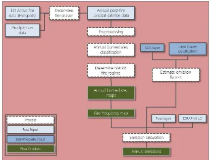
This report presents the results of Work Package 4 (WP 4): Historic fire regime.

(6)

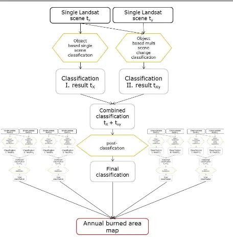
Figure 1: Workflow of the historic fire regime analysis

2.

Methodology

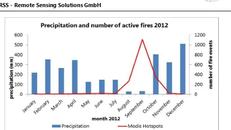
2.1 Selection of annual mid resolution images for the years 1990 – 2014

(7)

Figure 2: Example of a fire season analysis for a given year based on precipitation data and MODIS active fire data.

(8)

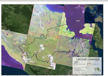
Figure 3: Five Landsat tiles are needed to cover the BIOCLIME project area.

(9)

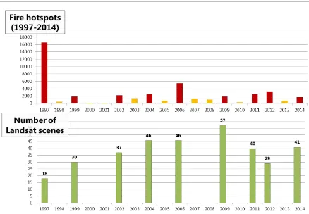
Figure 4: The upper diagram shows the number of MODIS hotspots within the BIOCLIME project area from 1997 to 2014. Red bars indicate the years selected for mapping, yellow bars indicate the years not mapped. The lower diagram depicts the number of considered Landsat scenes for the years mapped.

DATA LIMITATIONS:

(10)

Table 1: Technical features of the Landsat 5 sensor (Thematic Mapper (TM)

Landsat 5 (8bit) Thematic

Mapper (TM)

Bands _{(micrometers)}Wavelength Resolution_(meters)

Band 1 0.45-0.52 30

Band 2 0.52-0.60 30

Band 3 0.63-0.69 30

Band 4 0.76-0.90 30

Band 5 1.55-1.75 30

Band 6 10.40-12.50 120* (30)

Band 7 2.08-2.35 30

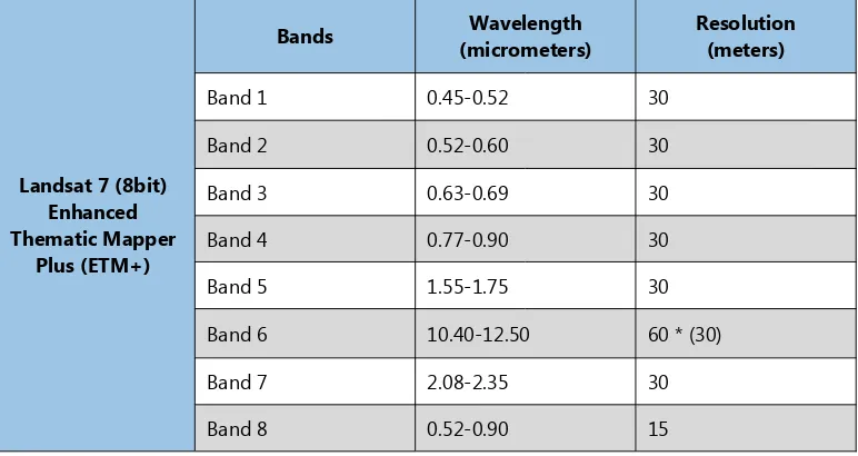
Table 2: Technical features of the Landsat 7 sensor (Enhanced Thematic Mapper plus (ETM+)

Landsat 7 (8bit) Enhanced Thematic Mapper

Plus (ETM+)

Band 1 0.45-0.52 30

Band 2 0.52-0.60 30

Band 3 0.63-0.69 30

Band 4 0.77-0.90 30

Band 5 1.55-1.75 30

Band 6 10.40-12.50 60 * (30)

Band 7 2.08-2.35 30

(11)

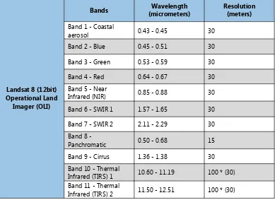
Table 3: Technical features of the Landsat 8 sensor (Operational Land Imager (OLI)

Landsat 8 (12bit) Operational Land

Imager (OLI)

Band 1 - Coastal

aerosol 0.43 - 0.45 30

Band 2 - Blue 0.45 - 0.51 30

Band 3 - Green 0.53 - 0.59 30

Band 4 - Red 0.64 - 0.67 30 Band 5 - Near

Infrared (NIR) 0.85 - 0.88 30 Band 6 - SWIR 1 1.57 - 1.65 30

Band 7 - SWIR 2 2.11 - 2.29 30 Band 8

-Panchromatic 0.50 - 0.68 15 Band 9 - Cirrus 1.36 - 1.38 30 Band 10 - Thermal

Infrared (TIRS) 1 10.60 - 11.19 100 * (30) Band 11 - Thermal

Infrared (TIRS) 2 11.50 - 12.51 100 * (30)

The spatial resolution of the optical bands and the SWIR (short wave infrared) bands used for classification is 30 meters.

The smallest feature that can be mapped is equal to one pixel (30 m x 30 m for Landsat data used in study). However, it is agreed upon that the smallest observable feature that can be reliably identified needs to consist of more than one contiguous pixels. The reason is that a feature with a size of only one pixel will almost never fall entirely within one pixel, but will instead be split across up to four pixels. Therefore, the feature’s reflectance would make up only a fraction of those pixels and thus could not be reliably classified. In order to avoid this effect, a Minimum Mapping Unit (MMU) of 0.5 ha was introduced, representing the smallest possible unit to map.

(12)

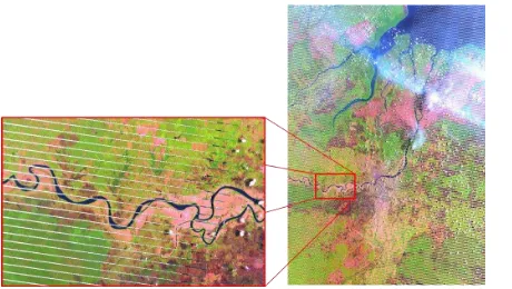
Figure 5: Landsat 7 SLC-off mode, data stripes.

A final constrain concerns the dependency of optical sensors on the atmospheric conditions. Clouds, haze and smoke hamper the opportunity to map burned areas, simply because the burned areas cannot be seen. These limitations were diminished using numerous overlapping scenes to be able to classify as many burned areas as possible.

2.2 Preprocessing: Radiometric and atmospheric correction

The pre-processing for Landsat data consisted of the removal of atmospheric distortions (scattering, illumination effects, adjacency effects), induced by water vapor and aerosols in the atmosphere, seasonally different illumination angles, etc. An atmospheric correction was applied to each image using the software ATCOR (Richter and Schläpfer 2014). This pre-processing step leads to a calibration of the data into an estimation of the surface reflectance without atmospheric distortion effects including topographic normalization. This calibration method facilitates a better scene-to-scene comparability of the radiometric measurements, which is a necessary precondition for the semi-automatic segment-based rule-set classification method applied in this study and the proposed monitoring system.

2.3 Image segmentation

The satellite images were then used as input for burned area classification using an object-based image analysis approach. The first step of the object-based approach is to generate so called “image-objects” which combines spatially adjacent and spectrally similar groups of pixels, rather than individual pixels of the image (pixel-based approach).

(13)

to high resolution satellite data and when mapping spectrally heterogeneous classes such as forest. The received signal frequency does not clearly indicate the membership to a land cover class, e.g. due to atmospheric scattering, mixed pixels, or the heterogeneity of natural land cover.

Improving the spatial resolution of remote sensing systems often results in increased complexity of the data. The representation of real world objects in the feature space is characterized by high variance of pixel values, hence statistical classification routines based on the spectral dimensions are limited and a greater emphasis must be placed on exploiting spatial and contextual attributes (Matsuyama 1987, Guindon 1997, 2000). To enhance classification, the use of spatial information inherent in such data was proposed and studied by many researchers (Atkinson and Lewis 2000).

Many approaches make use of the spatial dependence of adjacent pixels. Approved routines are the inclusion of texture information, the analysis of the (semi-)variogram, or region growing algorithms that evaluate the spectral resemblance of proximate pixels (Woodcock et al. 1988, Hay et al. 1996, Kartikeyan et al. 1998). In this context, the use of object-oriented classification methods on remote sensing data has gained immense popularity, and the idea behind it was subject to numerous investigations since the 1970’s (Kettig and Landgrebe 1976, Haralick and Joo 1986, Kartikeyan et al. 1995).

2.4 Mapping annual burned areas: spatial extent and fire severity

Burned areas were classified based on burn ratios (BR) of bands b0.84µm, b2.22µm, and b11.45µm: BR1 = (b0.84µm- b11.45µm) / (b0.84µm+ b11.45µm) (eq. 1) where b0.84µm is the reflectance value of Near Infrared (0.76-0.90 µm) and b11.45µm is the reflectance value of Thermal Infrared (10.4-12.5µm).

BR2 = (b0.84µm- b2.22µm) / (b0.84µm+ b11.45µm) (eq. 2) where b0.84µmis the reflectance value of Near Infrared (0.76-0.90 µm), b2.22µmis the reflectance value of Mid-Infrared (2.08-2.35 µm) and b11.45µmis the reflectance value of Thermal Infrared (10.4-12.5µm).

NBR = (b0.84µm- b2.22µm)/(b0.84µm+ b2.22µm) (eq. 3) where b0.84µmis the reflectance value of Near Infrared (0.76-0.90 µm) and b2.22µmis the reflectance value of Mid-Infrared (2.08-2.35 µm).

The Normalized Burn Ratio (NBR) was used to assess the fire intensity. The ratios BR1 and BR2 have already been successfully applied for burned area mapping in the province Riau, Sumatra (Baier 2014). Additionally, the normalized difference vegetation index (NDVI) was calculated to improve the detection of clouds, water and burned areas.

NDVI = (b0.84µm- b0.66µm)/(b0.84µm+ b0.66µm) (eq. 4) where b0.84µmis the reflectance value of Near Infrared (0.76-0.90 µm) and b0.66 µmis the reflectance value of red (0.64 - 0.67µm).

(14)

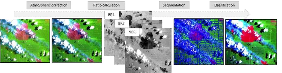
Figure 6: Processing steps from atmospheric correction of the Landsat data to the segmentation and finally the classification.

2.5 Mapping approaches

We combined two object-based approaches to overcome particular limitations of each single approach. Combining both outputs lead to the best results of burned area classification. After the automatic classification manual revision was necessary especially in areas with a lot of smoke and/or haze.

A water and cloud-mask was applied to all images before processing based on the normalized difference water index (NDWI) and Cloud-Index (based on the Quality Assessment band provided by USGS) in order to avoid misclassifications in water and cloud/cloud shadow areas.

NDWI = (b0.84µm– b1.57µm)/(b0.84µm+ b1.57µm) (eq. 5)

Where b0.84µm is the reflectance value of Near Infrared (0.76 - 0.90 µm) and b1.57µmis the reflectance value of Short Wave Infrared (1.57 – 1.65µm).

(15)

(16)

The following three paragraphs will explain the difference between the two approaches, their strength and limitations as well as the final combination of both.

1.1.1 Approach 1 - Object based classification based on single scene

In the single scene approach, burned areas were classified based on one Landsat scene utilizing the derived burn ratios described above. The settings for segmentation and classification enable the detection of small scale burned areas (little agricultural fields) to large scale forest fires.

Thresholds for classifying burned areas were defined by a variable approach based on Landsat image statistics. Fixed thresholds were used for all Landsat scenes, whereas they had to be adjusted for Landsat 8 and Landsat 5/7 due to slightly different wavelengths characteristics. As a last step, the MMU was applied and objects were smoothened.

LIMITATIONS:

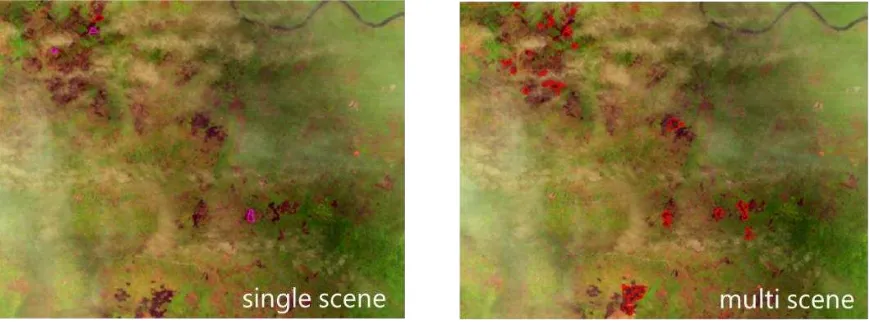
The main limitation of the single scene approach is the detection of burned areas in areas with haze. Even though the scenes were atmospherically corrected, the influence of thick haze and/or smoke cannot fully be diminished. Having numerous scenes with haze and or smoke (fire season) lead to the idea of combining this approach with a multi-temporal approach to overcome this limitation (see approach 2).

1.1.2 Approach 2 - Object based multi scene change detection (t1 – t2)

The multi scene approach is based on images with a maximum sensing difference of 32 days which were stacked and segmented based on the multiple spectral bands and the derived Indices (based on an approach by Melchioriet al.2014).

Burn areas were classified by the mean spectral values of an object for the change rate (CR) and the difference (D) CRNDVI, CRNBR, DNBR and NBR. Different thresholds (t) were used for Landsat 8 and Landsat 5/7. (eq. 6) (eq. 7) (eq. 8) (eq. 9) LIMITATIONS:

(17)

Figure 8: This figure depicts the limitations of the multi scene approach. Clouds in one of the time steps prevent a classification in the cloud free time step.

1.1.3 Combining Approach 1 & Approach 2

The final derived classification is a combination of these two approaches to grant high accuracy and diminish false positives. The aforementioned limitations of both approaches are reduced via the combination of both approaches (see Figure 7). Additionally, the selection of all available Landsat scenes (instead of one cloud free single scene) for classification increased the accuracy. Figure 9 displays a comparison of single scene and multi scene approach for burned area detection.

(18)

2.6 Pre-fire vegetation, area burned and fire frequency

The historic fire regime was analyzed in terms of pre-fire vegetation, fire frequency, and area burned. Fire frequency was evaluated by cumulative merging and intersection of the annual burned areas (see Figure 21). The land cover classification produced by ICRAF for the years 1990, 2000, 2005, 2010 and 2014 (see Work Package 1 (WP 1) was used in order to assess pre-fire land cover class. This helps the identification of the drivers of deforestation. Furthermore, this allows an estimation of the carbon emissions released by fire in South Sumatra since 1990.

Finally, a shapefile was generated containing the following attributes: fire frequency, year of fire(s), pre-fire land cover class and spatial extent (area).

2.7 Accuracy assessment

At the time this report was compiled, no historic reference data was available on burned areas. Therefore, an accuracy assessment could not be conducted.

2.8 Emissions calculation

To calculate the emissions by the fires for each year, the aboveground emissions and peat emissions were calculated. Summing these products up leads to total emissions for each single mapped year. We used the stratify & multiply approach to calculate carbon stock maps from the land cover classifications of Work Package 1 (WP 1) in combination with the local aboveground biomass values derived in Work Package 3 (WP 3), and intersected those carbon stock maps with the fire frequency map for the calculation of the emissions. Emissions are reported in tons of carbon (t C).

Using the stratify & multiply approach for emission calculation first a stratification needs to be applied. We used the ICRAF land cover classification v3 product. This dataset then is intersected with the burned area product of each single year mapped. Each stratum (in our case each land cover class) is attributed with an emission factor (aboveground biomass value) which was derived in WP 3 by using the LiDAR based aboveground biomass (AGB) model and the high spatial resolution land cover maps from Work Package 2 (WP 2). This increases the accuracy of the emissions drastically because the local variations of land cover and biomass directly feed into the emission calculations. To calculate the carbon content of a certain stratum, the biomass is simply divided by 2 (i.e. a carbon content of 0.5 is assumed). By multiplying the burned area with the carbon stock the carbon emissions from burning biomass are calculated.

In addition, the carbon emissions from peat burning were calculated. Peat stores huge amount of carbon and therefore leads to huge emissions when ignited. To calculate these emissions, we used the approach by Konecny et al. (2016), which discriminates between first, second and or more fires with regard to the peat burn depth, and therefore the amount of carbon which is released.

(19)

Figure 10: The peatland distribution within the BIOCLIME study area. Derived from the peatland distribution map for 2016 created by the Ministry of Environment and forestry (MoEF).

Burned areas within formerly forested peatlands are considered to be first-fires and therefore a burn depth of 17 cm is applied (see Konecny et al.2016). All other land cover classes are then assigned to second or more fires with a reduced burn depth. So we only discriminate two different stages of fires (first and second or more).

(20)

3.

Results

3.1 Burned area

Burned area maps for 9 different years (1997, 1999, 2002, 2004, 2006, 2009, 2011, 2012 and 2014) were generated (see Figure 11 to Figure 19). In addition, a burned area map for 2015 based on Sentinel-1 RADAR data was provided from the ESA (European Space Agency) funded Fire CCI (Climate Change Initiative) project, and was integrated into the analysis and results (see Figure 20).

(21)

(22)

(23)

(24)

(25)

(26)

(27)

(28)

(29)

(30)

[image:30.842.83.680.73.489.2]

(31)

[image:31.842.84.680.73.489.2]

(32)

[image:32.595.106.489.224.377.2]

Table 4 shows the number of satellite scenes used, the amount of hotspots detected and the total area burned for each year. For the years 1997 (333,931 ha) and 2015 (323,397 ha), by far, the most area burned was detected, with 1997 even higher than 2015.

Table 4: Statistical information about the classified years. Shown are the number of satellite scenes used, the amount of hotspots detected and the total area burned for each year.

Year No. Scenes Hotspots Total Area Burned [ha] Area Burnedon Peat [ha]

1997 18 16,573 333,931 202,920

1999 30 1,888 64,009 29,241

2002 37 2,216 119,204 43,985

2004 46 2,515 120,029 39,085

2006 46 5,494 243,560 113,897

2009 57 1,875 68,172 22,131

2011 40 2,592 89,310 49,358

2012 29 3,319 164,246 95,873

2014 41 1,755 53,440 25,565

[image:32.595.120.464.524.761.2]

2015 Sentinel-1 8,582 323,397 185,399

(33)

(34)

[image:34.595.67.523.121.338.2]

Figure 23: Graph depicting the number of MODIS Hotspots detected during the selected years within the BIOCLIME study area and the mapped burned area for each year in hectares.

3.2 Pre-fire vegetation

Figure 24 depicts the area burned per land cover class for each year.

In 1997 the share of burned primary forest is by far the biggest compared to the other years. 165,865 ha of “Primary swamp forest”, 17,710 ha of “Primary dry land forest” and also 3,282 ha of “Primary mangrove forest” burned in 1997. In total this sums up to 186,857 ha of burned primary forest in 1997. The second largest primary forest burning in the BIOCLIME project area took place in 2006 with only (compared to 1997) 17,133 ha of burned primary forest in total. The burning of the land cover class “Tree crop plantation” is increasing over the years and in 2015 more than 106,773 ha of it burned. The same increase over time is visible for the class “plantation forest” where more than 29,275 ha burned in 2015. There is a clear change in ratio of land cover classes burned over the last two decades.

(35)

[image:35.595.73.518.128.712.2]

(36)

3.3 Emissions

[image:36.595.69.517.255.712.2]

Table 5 depicts the aboveground carbon emissions for each mapped year, as well as the peat emissions and the total emissions in megatons of carbon (Mt C). The highest emissions were calculated for 1997 with 72.22 Mt C followed by 2015 with 24.84 Mt C, 2006 with 21.25 Mt C and 2012 with 10.25 Mt C. Further it is visible that emissions are not directly connected to the total burned area. This is also shown in Figure 25, where the X-Axis depicts the years, the Y-Axis the burned area in hectares and the diameter of the circles the amount of carbon emissions. It can be concluded that different land covers lead to different emissions, further the distribution of the peat layer also plays an important role in the amount of emissions.

Table 5: Emissions per year megatons of carbon (Mt C), split up into aboveground (above) and peat emissions.

Year Area burned(ha) AboveEmissions (Mt C)Peat Total

1997 333,931 51.87 20.36 72.22

1999 64,009 5.61 2.01 7.62

2002 119,204 5.18 2.96 8.13

2004 120,029 5.37 3.17 8.54

2006 243,561 11.80 9.45 21.25

2009 68,172 2.94 1.49 4.43

2011 89,310 3.56 3.64 7.20

2012 164,246 4.55 5.70 10.25

2014 53,440 1.51 1.67 3.18

2015 323,397 10.58 14.26 24.84

Total 1,579,297 102.96 64.71 167.67

(37)

[image:37.595.72.526.174.506.2]

Figure 26 displays the total emissions divided into aboveground and peat emissions in megatons of carbon (Mt C). this figure shows that the ratio of emissions from aboveground biomass to peat changes over time. In the past proportionally more emissions were from aboveground biomass burning whereas in recent years proportionally more emission from peat burning.

Figure 26: Total emissions divided into aboveground and peat emissions in megatons of carbon (Mt C). The light red bars depict the carbon emissions of the aboveground biomass (ABOVE) and the dark red bars the peat emissions (PEAT).

(38)

[image:38.595.144.455.146.288.2]

Table 6: The burned area per year within the land cover class "No data".

Year Area burned (ha) No data (ha) Percentage

1997 333,931 17,646 5.28%

1999 64,009 7,090 11.08%

2002 119,204 13,591 11.40%

2004 120,029 12,538 10.45%

2006 243,560 22,904 9.40%

2009 68,172 4,782 7.02%

2011 89,310 12,778 14.31%

2012 164,245 17,402 10.59%

2014 53,440 514 0.96%

2015 323,397 3,244 1.00%

Total 1,579,297 112,489 7.12%

4.

Conclusions

Following conclusions could be drawn (separated into burned area, carbon emissions from fires and ratio between carbon emission from aboveground biomass and peat burning).

Burned area

 A direct deduction of burned area from the amount of fire hotspots should always be treated with caution (only general trend).

 In 1997 the share of burned Primary Forest is by far the biggest.  The second largest Primary Forest burning took place in 2006.

 The burning of the land cover classes Tree Crop Plantation and Plantation Forest is increasing over the years.

 There is a clear change in ratio of land cover classes burned over the last two decades. Carbon emission from fires

 The years with the highest carbon emissions (megatons of carbon Mt C) from fire were:  1997 with 72.22 Mt C (megatons of carbon)

 2015 with 24.84 Mt C  2006 with 21.25 Mt C  2012 with 10.25 Mt C

 Emissions are not directly connected to the total burned area.

 Different land covers lead to different emissions, further the distribution of the peat layer also plays an important role in the amount of emissions.

Ration between carbon emissions from aboveground biomass and peat burning

 The ration of emissions from aboveground biomass to peat burning changes over time.  In the past proportionally more emissions from aboveground biomass burning.

(39)

5.

Outlook

A next step would be to harmonize results from the carbon plots (Work Package 3). As the aboveground biomass calculations derived by the experts from the Bogor Agricultural University (IPB) are based on more differentiated allometric equations (e.g. species specific) it is recommended to use these aboveground biomass estimates to calibrate the LiDAR based aboveground biomass model in Work Package 3, which would lead to revised local aboveground biomass values for the different vegetation classes. This consequently would lead to a recalculation of the aboveground fire emissions (also for Work Packages 1 and 2).

Outputs / deliverables

 Vector data of fire frequency combining the burned areas of the years 1997, 1999, 2002, 2004, 2006, 2009, 2011, 2012, 2014 and 2015 (.shp format)

(40)

References

Atkinson P., Lewis P. (2000). Geostatistical classification for remote sensing: an introduction. Comput. Geosci. 26, 361–371.

Baier S.R (2014). Brandflächenklassifizierung in Riau, Sumatra unter Verwendung mittelauflösender Fernerkundungsdaten. Master Thesis, Paris Lodron-University Salzburg.

Guindon B. (2000). Combining Diverse Spectral, Spatial and Contextual Attributes in Segment-Based Image Classification. ASPRS 2000 Annu. Conf. 1–5.

Guindon B. (1997). Computer-Based Aerial Image Understanding: A Review and Assessment of its Application to Planimetric Information Extraction from Very High Resolution Satellite Images. Can. J. Remote Sens. 23, 38–47.

Haralick R., Joo H. (1986). A Context Classifier. IEEE Trans. Geosci. Remote Sens. GE-24, 997–1007. Hay G.J., Niemann K.O., McLean G.F. (1996). An object-specific image-texture analysis of H-resolution

forest imagery. Remote Sens. Environ. 55, 108–122.

Kartikeyan B., Majumder K.L., Dasgupta A.R. (1995). An expert system for land cover classification. IEEE Trans. Geosci. Remote Sens. 33, 58–66.

Kartikeyan B., Sarkar A., Majumder K.L. (1998). A segmentation approach to classification of remote sensing imagery. Int. J. Remote Sens. 19, 1695–1709.

Kettig R., Landgrebe D. (1976). Classification of Multispectral Image Data by Extraction and Classification of Homogeneous Objects. IEEE Trans. Geosci. Electron. 14, 19–26.

Konecny K., Ballhorn U., Navratil P., Jubanski J., Page S.E., Tansey K., Hooijer A., Vernimmen R., Siegert F. (2016). Variable carbon losses from recurrent fires in drained tropical peatlands. Glob Change Biol, 22: 1469–1480.

Matsuyama T. (1987). Knowledge-Based Aerial Image Understanding Systems and Expert Systems for Image Processing. IEEE Trans. Geosci. Remote Sens. GE-25, 305–316.

Melchiori A.E., Setzer A., Morelli F., Libonati R., Cândido P.A., de Jesús S.C. (2014). A Landsat-TM/OLI algorithm for burned areas in the Brazilian Cerrado – preliminary results. VII International Conference on Forest Fire Research D.X. Viegas (Ed.).

Richter R., Schläper D. (2014). Atmospheric / Topographic Correction for Satellite Imagery. 1–238. Woodcock C.E., Strahler A.H., Jupp D.L.B. (1988). The use of variograms in remote sensing: I. Scene

(41)

Appendix A

Burned area per land cover class (ICRAF 1990) and year (1997 and 1999).

ICRAF 1990

1997

1999

BAPLAN LCC (translated from ICRAF)

area [ha]

Burned already

1997 [ha]

burned area

[ha]

Tree crop plantation

28,158

15,564

1,478

14,086

Dry land agriculture

320

63

13

51

Embankment

0

Grass

12,119

2,621

733

1,889

Mixed dryland agriculture/mixed garden

3,298

2,498

451

2,047

No data

17,646

7,090

905

6,185

Open land

1,436

155

61

95

Plantation forest

0

Primary dry land forest

17,710

9,924

1,565

8,359

Primary mangrove forest

3,282

195

36

159

Primary swamp forest

165,865

11,503

2,943

8,559

Rice fields

15,702

4,609

1,203

3,406

Scrub

10,920

2,103

599

1,504

Secondary/ logged over swamp forest

46,056

5,220

1,600

3,621

Secondary/ logged over dry land forest

3,596

860

79

781

Secondary/ logged over mangrove forest

408

32

3

29

Settlement/ developed land

412

100

28

72

Water body

7,002

1,471

257

1,214

(42)

ICRAF 2000

2002

2004

area [ha]

Burned already

2002 [ha]

burned area

[ha]

42,482

45,962

5,275

40,687

128

94

8

86

Embankment

5

25

2

23

Grass

3,022

1,109

283

826

4,135

2,295

342

1,953

No data

13,591

12,538

1,242

11,296

Open land

3,154

2,923

747

2,176

Plantation forest

248

314

7

307

Primary dry land forest

765

704

10

694

366

170

26

144

Primary swamp forest

7,867

9,933

1,288

8,645

Rice fields

13,106

5,812

1,770

4,041

Scrub

11,071

6,376

1,521

4,855

12,574

26,191

2,596

23,595

2,296

2,157

54

2,102

191

184

15

169

986

1,029

278

751

Water body

3,217

2,212

314

1,898

(43)

ICRAF 2005

2006

2009

BAPLAN LCC (translated from ICRAF)

area [ha]

Burned already

2006 [ha]

burned area

[ha]

90,159

31,863

5,692

26,171

1,198

309

46

263

Embankment

1

0

Grass

2,177

550

138

412

9,634

2,531

546

1,986

No data

22,931

4,787

929

3,859

Open land

2,112

738

138

600

Plantation forest

6,179

2,155

344

1,811

883

904

8

897

183

64

44

20

16,068

4,935

1,048

3,887

Rice fields

10,276

2,643

535

2,109

Scrub

12,071

3,595

1,562

2,034

57,358

8,695

2,902

5,793

6,969

2,816

170

2,646

89

122

8

114

1,424

381

106

275

Water body

3,849

1,083

240

843

(44)

ICRAF 2010

2011

2012

area [ha]

Burned already

2011 [ha]

burned area

[ha]

34,422

70,338

5,130

65,208

2,081

4,598

503

4,094

Embankment

8

61

1

60

Grass

3,115

9,728

691

9,037

1,570

3,189

231

2,958

No data

12,778

17,402

1,637

15,765

Open land

370

1,090

111

978

Plantation forest

2,237

5,988

280

5,708

80

52

2

50

18

108

0

108

5,351

4,362

540

3,821

Rice fields

2,702

14,914

847

14,067

Scrub

6,211

9,717

1,390

8,326

14,513

13,074

1,335

11,739

1,610

3,565

148

3,417

207

366

20

345

710

1,572

120

1,453

Water body

1,326

4,123

178

3,946

(45)

ICRAF 2014

2014

2015

area [ha]

Burned already

2014 [ha]

burned area

[ha]

21,981

106,773

3,373

103,400

20

99

1

97

Embankment

104

415

3

413

Grass

1,375

6,130

155

5,974

1,940

5,351

113

5,238

No data

514

3,244

66

3,178

Open land

4,035

11,638

464

11,174

Plantation forest

4,876

29,276

1,207

28,068

85

87

2

85

116

1,753

29

1,724

288

2,988

29

2,959

Rice fields

4,413

13,948

695

13,253

Scrub

4,415

38,699

1,352

37,347

6,301

83,646

1,702

81,945

659

3,722

48

3,674

557

3,081

287

2,794

728

3,425

83

3,342

Water body

1,030

9,122

180

8,942