www.elsevier.com / locate / econbase
Irreversible investment under uncertainty and the threat of
bankruptcy
*
James Vercammen
University of British Columbia and University of Melbourne, Faculty of Commerce and Business Administration, 2053 Main Mall, University of British Columbia, Vancouver, British Columbia, Canada V6T 1Z2
Received 30 December 1998; accepted 14 June 1999
Abstract
The firm-level theory of irreversible investment under uncertainty is extended to account for bankruptcy. With a sufficiently large risk of bankruptcy, firms prefer to defer their investment decision to a later date. Simulated option values reach as high as 30 percent. 2000 Elsevier Science S.A. All rights reserved.
Keywords: Irreversible investment; Bankruptcy; Option value
JEL classification: D81; D92
1. Introduction
The literature on firm-level investment with irreversibility and uncertainty has grown rapidly over the last decade. The standard problem, first examined by McDonald and Siegal (1986), is comprised of a firm who must decide when to invest a fixed amount P in exchange for a project with value V where V is continually changing over time. The decision to invest is irreversible and thus an option value associated with waiting normally exists. That is, P must be sufficiently less than V in order for the investment to occur.
There have been many extensions of this basic model, much of which is described by Dixit and Pindyck (1994). For example, Leahy (1993) and others have examined option values in the context of a competitive equilibrium. Recent papers on irreversible investment under uncertainty and oligopoly include Fatas and Metrick (1997) and Baldursson (1998). Dixit (1991) examined the problem in the context of price ceilings and Dixit (1995) considered the role of scale economies. Sequential
*Corresponding author. Tel.: 001-604-822-5667; fax: 001-604-822-2184.
E-mail address: [email protected] (J. Vercammen)
investment and incremental investment have also been considered in several studies. Finally, Chang (1988) examines how irreversible investment impacts the incentive for horizontal merger.
Despite its importance for the decision making of most firms, bankruptcy has not yet been formally examined in the context of irreversible investment. Specifically, suppose in the standard model, the firm must borrow funds to finance the investment. If the firm is unlucky, outstanding debt may increase and exceed the value of the collateralized investment asset. At this point, the lender will foreclose by seizing the asset and the firm will lose access to the future revenue stream. Making an investment increases the probability of foreclosure. Therefore, waiting to invest may be valuable because waiting allows the firm to reduce its debt and also to avoid the investment if the risk of foreclosure increases.
The purpose of this paper is to develop a simple model of irreversible investment with foreclosure risk. To isolate the option value solely attributable to foreclosure risk, the model is constructed such that an option value does not exist in the absence of bankruptcy considerations. The normal assumption is that the value of the project follows some type of Brownian motion stochastic process. Suppose instead that returns are continuously and independently normally distributed. In the standard model, there is no value from waiting if the project’s value is stationary over time. Thus, any option value arising within the current model is due to the foreclosure risk.
An important assumption within the model concerns the form of the foreclosure rule. The standard rule, ‘foreclose if the firm becomes insolvent (i.e., outstanding debt exceeds the collateralized value of the assets),’ is employed. This rule is not necessarily efficient because an insolvent firm may expect to
1
eventually become solvent if it is allowed to continue operating . In this model, returns are stationary and the project is assumed profitable at date 0, implying that foreclosure is always inefficient / premature. However, lending without foreclosure (in which case the option value results of this paper vanish) would typically require an unbounded risk premium within the lending rate. For institutional
2
and transaction cost reasons, lenders typically do not employ this strategy .
2. The model
At time 0 a firm owns a plant (financed partially with debt) that continuously generates a stochastic level of net returns. These returns are independently and normally distributed with mean R and standard deviations. The plant cannot be sold until time T, at which point its value is P. If bankruptcy occurs prior to time T, the value of the plant to the foreclosing lender is also P. At time 0 the firm’s outstanding debt is D0,P. The lender can instantly and costlessly foreclose (i.e., seize and resell the
plant) and thus bears no risk because the following rule is assumed: ‘foreclose instantly if outstanding debt rises to level P’. Consequently, the interest rate set by the lender, r, equals the risk-free cost of
1
If inefficient foreclosure is interpreted as a bankruptcy cost, then the results of this paper are still consistent with the Modigliani and Miller theorem. In the absence of bankruptcy costs, this theorem implies that, regardless of the level of debt, a firm’s investment reserve price equals the discounted presented value of expected returns.
2
capital, which is also equal to the firm’s discount rate. If foreclosure occurs, the firm’s net profit at time T equals zero with certainty.
1
At either time 0 or time t (an exogenous parameter) the firm can invest in an identical plant at cost
P. This new plant, which generates net returns identical to the original plant, also has a time T salvage
value for the firm and value for a foreclosing lender equal to P. If the investment is made, the cost must be completely debt financed. The firm is assumed to continuously contribute all net returns toward outstanding debt since its objective is to maximize expected equity at time T. Therefore, outstanding debt, D(t), has the following continuous time stochastic structure:
dD5srD2iR dtd 1isdz (1)
where i[h1, 2jdenotes the number of plants operated by the firm and dz is the increment of a Wiener
3 1 the value of each plant is P. This probability function is evaluated as of time t. The corresponding
i i 1
density function,≠H (t;t, D, P) /≠t, is denoted h (t;t, D, P). Let g(D; t , D , P) denote the probability0
1
density function for outstanding debt at time t evaluated as of time 0 given initial debt D and plant0 value P. Explicit equations for these two functions are specified below.
1
Let W(D,t, P) witht[h0, t jdenote the timet value of the expected contribution of the additional plant to time T equity given outstanding debt at time t equal to D, plant value P and i51. An expression for W(D,t, P) can be written as
T
(strictly) positive incentive to invest in the additional plant, even if the probability of bankruptcy was zero. Such a case is uninteresting and is therefore assumed away.
The top (bottom) half of Eq. (2) is the expected surplus when operating two plants (one plant). The difference, therefore, is the expected equity contribution of the additional plant. The first term in each half of Eq. (2), V(12exp(2r[T2t])), equals the present value of additional expected equity if the risk of foreclosure equals zero. The term V(exp(r[T2t])21) equals the expected loss in time T
]
3 Œ
4
equity if foreclosure occurs at time t . This term is multiplied by the probability of foreclosure at time
t, integrated over time and then discounted to timet to obtain the total expected loss in equity for the firm attributable to the inefficiency of the foreclosure rule. It is convenient to rewrite Eq. (2) as
R
Suppose the firm does not invest in the additional plant at time 0. At time t the investment will be
1 1 1
It follows that the firm will only invest in the additional plant at time 0 if P satisfies W(D , 0,0
1
P)$C(D , t , P).0
i
To complete the analysis, it is necessary to specify expressions for the two density functions, h (t;t,
1
D, P) and g(D; t , D , P). Unfortunately, such expressions are unknown when debt evolves according0 i
5 ˆ 1
ˆ
to Eq. (1) . Approximations of these two functions, denoted h (t; t, D, P) and g(D; t , D , P),0
respectively, can be derived as follows. Rewrite Eq. (1) as
ˆ
dD5dD1r
f
D2D02(i21)P dt,g
(5)where
ˆ ˆ
dD5
s f
rD01(i21)Pg
2iR dtd
1isdz with D(0)5D(0)5D01(i21)P. (6)Eq. (6) is a Brownian motion with drift stochastic process. Formulas for first hitting times and
ˆ
probability densities are well known for this process (e.g., Ingersoll, 1987, pp. 352–353). Thus if D is
i 1
Suppose for the case of i51 that D(t)5P (i.e., the firm is insolvent at time t). If the firm was allowed to continue
operating, debt is expected to fall below P over time since R.rP. Foreclosure implies that this expected increase in equity
cannot be captured. The time T size of the loss in expected equity when foreclosure occurs at time t is measured by the term
V(exp(r[T2t])21).
5 1
1 1 1 2
wheref(?; ?,?) denotes the probability density function for a normal random variable with mean and
6
variance given by the last two arguments, respectively .
3. Solution and simulation results
Attention is restricted to the case corresponding to G(D , 0, P)0 $0 in Eq. (3). That is, the probability of foreclosure is not excessive such that a firm with a now-or-never investment option at
7 1
time 0 chooses to exercise the option . The firm prefers to defer the investment decision to time t
1
foreclosure. However, deferring investment has two benefits that may or may not offset the loss just
1
described. First, as Eq. (4) shows, the firm has the option of not investing at time t if net returns are
1 1
sufficiently poor between time 0 and time t . This truncation increases the expected value of W(D, t ,
1
P). Second, if the investment is deferred, debt is expected to decrease below D from time 0 to time t0
because R.rP. Eq. (3) shows that this expected decrease in debt will increase the expected value of
1 1 2 1
W(D, t , P) provided thatG(D, t , P) is decreasing in debt. This condition holds because 2h (t; t , D,
1 1
P)2h (t; t , D, P) is increasing in debt (i.e., the contribution toward foreclosure risk from the
additional investment is greater at higher levels of debt).
1
If the risk of foreclosure is sufficiently high such thatC(D , t , P)0 .W(D , 0, P), then, in order for0
the firm to choose to invest at time 0, the cost of the investment, P, must be reduced. Let P* equal the
1 1
solution toC(D , t , P)0 5W(D , 0, P). P*0 5R /r is always a solution sinceC(D , t , R /0 r)5W(D , 0,0 1
R /r)50. The more interesting solution occurs whereC(D , t , P)0 .W(D , 0, P) for some P0 ,R /r. In this case, P*,R /r and P* now defines a non-trivial critical investment price. For P#P*, the firm
1
will invest at time 0 and for P.P*, the firm will defer the investment decision to time t . Another
interpretation is that R /r2P* is a measure of the size of the investment option.
To obtain simulation results, Eqs. (7) and (8) must be substituted into Eqs. (3) and (4) and the integrals evaluated. Unfortunately, analytical solutions for these integrals cannot be obtained so
8
numerical integration techniques must be employed . An iterative numerical algorithm based on the procedure described above was used to obtain the solution value, P*, for a variety of parameter combinations. Sensitivity analysis (not reported) ensured that each solution is globally stable. The fixed parameters of the model were set as follows: T510, r50.1, and R51. The remaining
6
The two approximations implied by Eqs. (7) and (8) will result in an underestimate of the value of the option. Contact the author for the proof.
7
It is easy to establish that option values due to foreclosure risk also arise for the case where G(D , 0, P)0 ,0.
8
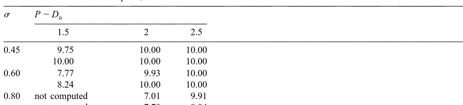
Table 1
a
Simulated critical investment price, P*
s P2D0
1.5 2 2.5
0.45 9.75 10.00 10.00
10.00 10.00 10.00
0.60 7.77 9.93 10.00
8.24 10.00 10.00
0.80 not computed 7.01 9.91
not computed 7.79 9.94
a 1 1
Solution values at top (bottom) of each row correspond to t 51 (t 52). Values for the other parameters arer 50.1,
T510 and R51.
1
parameters, t ,s, and initial equity (P2D ), were varied as shown in Table 1. Note that the top half0
1 2
of each row of results corresponds to t 51 and the bottom half to t 52.
With R51 and r50.1, the riskless critical investment price for the firm equals (R51) /(r5
0.1)510. Because R51, the row labels can also be interpreted as coefficient of variation parameters. Similarly, because P*¯10, the column labels (multiplied by 10) can also be interpreted as approximate initial equity to asset percentages. A solution value for the cell at the extreme bottom left of Table 1 has not been computed because with this parameter combination, G(D , 0, P)0 ,0 and the analysis does not cover this case.
The results are consistent with the earlier discussion. If the risk of foreclosure is comparatively low (toward the top right of Table 1), then the option to defer investment has zero value and the firm is willing to pay price R /r510 for the additional plant at time 0. On the other hand, with a high risk of foreclosure (toward the bottom left of Table 1), the option to defer investment has positive value such that the critical purchase price, P*, is discounted below R /r510. Notice that the discounts can be sizeable (e.g., 20 to 30 percent) for levels of risk and debt ratios that are certainly high yet not likely outside a feasible operating range for some firms. Finally, notice that the price discounts are reduced
1 1
when t is increased from 1 to 2. This result suggests that t 52 is sub-optimally long from the firm’s perspective.
4. Concluding remarks
process, it is likely that stronger results would be obtained because the foreclosure rule would be relatively less efficient in such a case.
Acknowledgements
Financial support from the Social Science and Humanities Research Council of Canada and the Faculty of Economics and Commerce at the University of Melbourne is gratefully acknowledged.
References
Baldursson, F.M., 1998. Irreversible investment under uncertainty in oligopoly. Journal of Economic Dynamics and Control 22, 627–644.
Chang, M., Harrington, J., 1988. The Effects of Irreversible Investment in Durable Capacity on the Incentive for Horizontal Merger. Southern Economic Journal 55, 443–453.
Dixit, A., 1991. Irreversible investment with price ceilings. Journal of Political Economy 99, 541–557.
Dixit, A., 1995. Irreversible investment with uncertainty and scale economies. Journal of Economic Dynamics and Control 19, 327–350.
Dixit, A., Pindyck, R., 1994. Investment Under Uncertainty, Princeton University Press, Princeton, New Jersey. Fatas, A., Metrick, A., 1997. Irreversible investment and strategic interaction. Economica 64, 31–47.
Ingersoll, J.E., 1987. Theory of Financial Decision Making, Rowman and Littlefield, New Jersey.
Leahy, J.V., 1993. Investment in competitive equilibrium: the optimality of myopic behaviour. Quarterly Journal of Economics 108, 1105–1133.