ANALYSIS
The impact of remanufacturing in the economy
Geraldo Ferrer
a,*, Robert U. Ayres
baThe Kenan-Flagler Business School,The Uni6ersity of North Carolina at Chapel Hill,Chapel Hill,NC27599-3490,USA bINSEAD,Bl6d.Constance,F-77305Fontainebleau,France
Received 28 December 1998; received in revised form 28 June 1999; accepted 4 August 1999
Abstract
Very few durable goods are recovered at the end of their useful lives. However, this situation could reverse with the development of a stronger remanufacturing industry in the economy. This paper evaluates the impact of remanufac-turing in a hypothetical situation where remanufacremanufac-turing holds a significant share of the economy, presently dominated by the original manufacturing industries. We adapt the inter-industry input – output framework with the development of a methodology to consider these changes. Subsequently, we apply the model to the 30-sector aggregation of the French input – output national data to illustrate the method and to evaluate the impact that remanufacturing may have on the economy. Remanufacturing sectors substitute labor and transport services for the usual inputs such as raw materials and semi-finished goods. We find that remanufacturing may satisfy the same final demand from all sectors requiring fewer intermediate resources. Consequently, the economy observes proportionally higher demand for labor and all other products. © 2000 Elsevier Science B.V. All rights reserved.
Keywords:Remanufacturing; Product recovery; Inter-industry flows; Input – output model; France
www.elsevier.com/locate/ecolecon
1. Introduction
The production of durable goods represents an important contribution to the GNP of all devel-oped countries. It employs large amounts of hu-man resources, raw materials and energy. However, most of the resources consumed are not renewable. The minerals that provide most of the raw materials and energy in the production of
durable goods have been continually depleted. Moreover, many durable products are disposed in landfills at the end of their useful lives without undergoing any recovery process. The landfill space has been decreasing and the prices charged by the landfills still in operation have increased very rapidly.
Ayres et al. (1997) suggested that remanufactur-ing is one approach to deal with the used durable goods at the time of disposal because of two first-order effects. In the production side, remanu-facturing reduces the demand for raw materials since part of the production is assured by the
* Corresponding author. Fax: +1-919-9626949.
E-mail addresses: geraldo –[email protected] (G. Ferrer), [email protected] (R.U. Ayres)
recovery of used goods: it is the resource conser-vation effect. In the disposal side, remanufactur-ing provides an alternative stream for used durable goods at the end of their useful lives. It reduces the amount of landfilled material given that significant fractions of the durable goods are reused: it is the waste reduction effect. Remanu-facturing is bound by limitations that should not be ignored. Ferrer (1997b) proposes methods to manage a large population of tires in a commer-cial fleet, including new and retreaded tire. That study highlights losses inherent to material fatigue and recovery yields. In related research, Ferrer (1997a) proposes criteria for remanufacturing and upgrading personal computers. In that case, the limitations are related to technology development and obsolescence.
Today, there are two major structural limita-tions precluding the expansion of remanufactur-ing activities. The existremanufactur-ing infrastructure is not suitable for the return flow, and most products arriving at the end of the first useful life are not designed for remanufacturing. This situation may change. Manufacturers are more conscious of their responsibility regarding product disposal, and are considering the adoption of Design for the Environment (DFE). In addition, changes in legislation may require manufacturers (or im-porters) to take back the carcasses of end-of-life automobiles, electronic goods and other durable products for responsible disposal or, preferably, recovery. Consequently, when the industry adopts efficient reverse logistics and design for the envi-ronment, one may see a substantial increase in the remanufacturing activity, even if regulation fails to require it. Since remanufacturing affects the level of consumption of several inputs (raw mate-rials, labor and energy), it will have significant impact on the economy, as it becomes a general-ized practice.
The remanufacturing success stories available today (photocopiers, tire retreading) represent a tiny fraction of economic activity. Thus, we can-not be certain about their second-order effects. For example, intuition says that the reduction in the consumption of raw materials reduces the demand from utility suppliers and machinery manufacturers. Likewise, employment is reduced
in the same industries. Nevertheless, it is hard to guess what direction total employment will take, since remanufacturing is also a labor-intensive activity. Original manufacturing (usually mass production) is much more able to capture economies of scale than remanufacturing. Due to heterogeneous inputs, the typical production rule adopts small lots. Also, disassembly is inherently more labor intensive, and less amenable to au-tomation than is assembly. These questions have to be dealt with carefully in order to understand if remanufacturing is an activity to be supported by governmental action or not.
In this paper, we develop a model for evaluat-ing the economic impact of a generalized product recovery and remanufacturing activity. The ma-trix of inter-industry transactions is augmented to incorporate the remanufacturing sector. It is adapted to recognize the different demands in labor, energy, raw materials, and inputs from the other industries. A basic assumption is that the final demand (in physical units) from remanufac-turing and from original manufacremanufac-turing remains the same as in the original scenario. In addition, it is assumed that the remanufactured product is sold at a price lower than that of a new good. This drives the first-order effect of implementing remanufacturing. However, the higher-order ef-fects are harder to estimate, but the methodology in this paper allows the identification of their impact.
Key questions are: what would happen if durable goods, such as automobiles, trucks, televi-sions and personal computers, were substantially remanufactured? How would it affect the demand for the traditional inputs in these industries? How would the massive presence of remanufactured goods affect the demand for raw materials? Some of the inputs, like energy and semi-finished goods, are expected to decline but labor utilization might increase. The main contribution of this paper is to generate the methodology that enables answering these questions. In order to decide on the imple-mentation of take-back regulations, policy makers and industrial lobbies need to understand the consequences of such decisions in the whole economy.
how to disaggregate sectors in aggregated tables using the methodology first described by Wolsky (1984). Section 3 adapts Wolsky’s methodology to introduce a new sector in the input – output table, the remanufacturing industry. Section 4 uses the methodology developed in this paper to evaluate the impact of remanufactured products in the economy.
2. The input – output methodology
Leontief (1936) first developed the input – out-put model as an analytical framework describing the interdependence of different industrial sectors. The model requires the preparation of an econ-omy-wide table, generally compiled by the statisti-cal agency of the national government. Each entry in the table corresponds to the sales from a given industrial sector to another industrial sector. One fundamental assumption in the framework is that the production function of all industries is linear. That is, if the total output of a given sector is increased, its consumption from (or payments to) all other sectors is increased in the same propor-tion. This implies that the technical coefficients are the fixed set of parameters under which the economy operates. Another assumption is that the technical coefficients do not change unless there is some change in the technology employed in one or more sectors. In practice, technological changes do occur in most sectors every period. One should expect to find different matrices of technical coefficients each year, reflecting these changes.
The input – output model has been extensively used to evaluate the impact of structural changes in the economy. Some have used this model to evaluate the changes due to the increased con-sumption of a given commodity, as in Davis (1987) and Howell (1985). Others have used it to evaluate the implication of environmental control policies, such as Hannan and Rose (1988), Lee (1982), Lowe (1979) and Rhee and Miranowski (1984). Finally, some have evaluated the dynamic changes in a given economy using the input – out-put tables of successive years, as in Driver (1994), and Feldman et al. (1987). In what follows, we
show the basic mathematics used in this type of evaluation.
Consider an input – output table as just de-scribed. Let Z be then×n matrix of inter-indus-try transactions, Y the column vector of final demands and X the column vector of total out-puts. For any sector i, by construction,
Xi=Zi1+Zi2+…+Zin+Yi
This expression corresponds to the sum of all sales made by sector i in the economy. Each Zij
element in the right-hand side corresponds to the inter-industry sales from sector i to sector j. Let Aij be the ratio between each element Zij and the
total output of the sector j, Xj. That is
Aij=Zij/Xj
This generates the matrix of technical coeffi-cients, A. Eliminating Z from both sets of equa-tions, we obtain the expression
(I−A)X=Y
In general, the matrix (I−A) is nonsingular, that is, its determinant is not zero. Hence:
X=(I−A)-1
Y
The main difficulty using input – output tables is to adapt the tables generally made available by official sources into one that contains the sectors that we want to analyze. This adaptation requires two sets of operations: sector aggregation and sector disaggregation. In this paper, we limit the size of the problem using a 30-sector aggregation of the French national economy.
2.1. Disaggregating input–output tables
origi-nally prepared. A number of researchers have worked on the problem of disaggregating input – output tables. The work by Wolsky (1984) deals precisely with it.
Let A and B be two technical coefficient ma-trices of the same economy, whereA is the n×n matrix obtained from the aggregation of matrix
B, a (n+1)×(n+1) matrix. For simplicity of exposition, the firstn−1 sectors in both matrices are the same. The nth sector in matrix A is the aggregation of the last two sectors in matrix B. Hence, each element in matrix A relates to the elements in B as follows:
A=
wherep(orq, respectively) is the ratio of the total output from sectorn (or sector n+1) to the sum of the total output of sectors n and (n+1). This operation allows defining the aggregated matrixA
from a larger matrix B. One may use this set of equations to aggregate related sectors that are not directly involved in the analysis. (For example, in this paper, in order to facilitate the evaluation of the remanufacturing effects in the economy, we aggregate some sectors that are not strongly re-lated with the manufacture or utilization of durable goods.)
However, if one wishes to obtain the disaggre-gated matrix B from the smaller matrix A, one will find that the system is underspecified. Any given n×n matrix, has several (n+1)×(n+1) matrices satisfying this set of equations. Wolsky approached this problem by introducing theaug -mentedand distinguishing matrices. The disaggre-gated matrix (B) is the sum of the augmented (H) and the distinguishing (D) matrices.
The augmented matrix H is one of the many (n+1)×(n+1) matrices satisfying the set of equations above. It is defined as the one matrix where sectorsnandn+1 require the same inputs, controlling market shares of pandq, respectively.
H=
The auxiliary matrices that are pre- and post-multiplying matrix A are the same appearing in Eq. (1), operating in the opposite order. The operation can be easily generalized to situations when one wishes to perform multiple disaggrega-tions. The augmented matrix considers sectors n and n+1 as essentially the same. The disaggre-gated matrix, however, must reflect the different inputs and outputs of these sectors. This distinc-tion is obtained with the distinguishing matrix. Once we perform the matrix operation in (2), we must identify the parameters that characterize the distinguishing matrixD. Let iBnandjBn desig-nate any of the (n−1)×(n−1) elements in ma-trix A that is identical to the corresponding elements in the larger matrixB. Since,D=B−H, and Bij=Hij=Aij, we obtain
[Dij=0, ÖiBn, jBn (3)
The nth and the (n+1)th rows in the aug-mented matrix presume that the market share across all columns is the same. This condition is relaxed with the corresponding rows in the D
Á Ã Í Ã Ä
Bnj+Bn+1j=Anj
pAnj=Hnj
qAnj=Hn+1,j
rArr;Dnj= −Dn+1,j (4)
Also, the nth and the (n+1)th columns in the augmented matrix are identical, presuming that both sectors use the same technology. The corre-sponding column in matrix D relaxes this condition.
!
pBin+qBi,n+1=AinHin=Hi,n+1=Ain
[
!
Din=q(Bin−Bi,n+1)Di,n+1=p(Bi,n+1−Bi,n)
[ (5)
Finally, the four elements in the lower-right corner of H incorporate both conditions men-tioned above. The corresponding elements in D
relax them as follows.
Notice that, since each Hin=Hi,n+1, than Bin−
Bi,n+1=Din−Di,n+1. Hence, the distinguishing
matrixDis completely defined withn−1 parame-ters to differentiate the last two rows, n−1 parameters to differentiate the last two columns, and three parameters to differentiate the four elements in the lower-right corner.
The row-differentiating parameters, call themsj,
indicate how much sector j departs from the average in its demand from sectorn. They satisfy Eq. (4). The column-differentiating parameters, call themdi, reflect the difference between sectors
nandn+1 in their demand for inputs from sector i. They satisfy Eq. (5). Parameterssnanddnsatisfy
Eq. (6) and serve the row- and column-differenti-ating functions. Parameter egives one additional degree of freedom, allowing full distinction
be-tween the sectors. Hence, the distinguishing ma-trix becomes:
DW=
Æ Ã Ã Ã Ã Ã È
0 0 ··· qd1 −pd1
0 0 qd2 −pd2 · ··
s1 sn+q(dn+e) sn−p(dn+e)
−s1 ··· −sn+q(dn−e) −sn−q(dn−e)
Ç Ã Ã Ã Ã Ã É
(7)
The development of the distinguishing matrix, due to Wolsky, allows for the disaggregation of two sectors previously aggregated in the input – output tables. For example, to evaluate the effect of substituting copper cables for aluminum cables, one could use Wolsky’s methodology to disaggre-gate thenonferrous metalssector into three sectors (aluminum, copper and other nonferrous metals). We use this methodology as a first-step to
intro-duce the remanufacturing corresponding to an original manufacturing industry in the input – out-put matrix.
3. Comparing remanufacturing and manufacturing activities
Remanufacturing is the process where a used durable good is disassembled at the module or at the component level, to repair or substitute com-ponents and modules that are worn out or obso-lete. In addition, the whole equipment is refurbished and critical modules are overhauled or substituted. A machine of today is built on yesterday’s base, receiving all the enhancements, expected life and warranty of a new machine. One
Á Ã Í Ã Ä
p(Bnn+Bn+1,n)+q(Bn,n+1+Bn+1,n+1)=Ann
Hnn=Hn,n+1=pAnn
Hn+1,n=Hn+1,n+1=qAnn
[ Á Ã Í Ã Ä
Dnn+Dn+1,n=q(Bnn−Bn,n+1)
+q(Bn+1,n−Bn+1,n+1)Dn,n+1+Dn+1,n+1=p(Bn,n+1−Bnn)
+p(Bn+1,n+1−Bn+1,n)Dn,n+1+Dn+1,n= −(Dnn+Dn+1,n+1)
interesting advantage that often occurs with re-manufactured goods is that several bugs that eventually existed in the original design are elimi-nated. Components in a remanufactured product tend to have much lower infant mortality than in an originally manufactured product. On the other hand, it is clear that components subjected to stress will have accumulated some fatigue — mi-croscopic fractures that gradually compromise its performance. However, the reduction in the ex-pected life of non-critical components often does not affect the expected life of the whole. It is the slack in expected life of valuable components that makes remanufacturing technically viable.
Remanufacturing has many similarities with the original manufacturing process. It also has some important differences. For the purpose of this study, we are interested in the difference between the inputs and the outputs of corresponding in-dustries. For example, what is the difference be-tween the inputs of tire manufacturing plants and tire retreading plants? What sectors absorb the output of one industry or another? The answer to this type of question is in the distinguishing ma-trix, specific for the input – output analysis when a new sector is introduced. The characteristics of the distinguishing matrix change significantly in our problem. Wolsky developed a method for disaggregating two industries operating indepen-dently in the same sector. Here, we would like to adapt it to analyze the introduction of the reman-ufacturing sector competing against an existing manufacturing industry, absorbing part of the market currently served by the original sector.
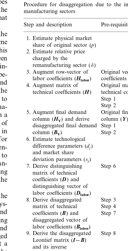
Table 1 lists the steps necessary to initiate the analysis. It starts with the estimation of the phys-ical market share of the original sector (p), and the relative price charged by the remanufacturing sector (dB1). We assume that the final demand for the product (in physical units) is not changed and that the remanufactured product is sold at a lower price. Let Yn be the final demand from the
original sector, in monetary units, before the in-troduction of remanufacturing. By construction, the new final demand from the original manufac-turing sector becomes p*Yn.
Defined as the ratio between the average prices
of remanufactured and originally manufactured
product. If the demand from the remanufacturing sector is q*Yn, it follows that q=d*(1−p). In
words, p and q are the monetary fraction of the original market held by the original manufactur-ing and the remanufacturmanufactur-ing sectors, respectively. Notice that reduced price in the new sector and constant physical output imply that p+qB1. Consequently, the sum of final demands from both sectors is reduced.
Table 1
Procedure for disaggregation due to the introduction of re-manufacturing sectors
Pre-requisites Step and description
1. Estimate physical market share of original sector (p) 2. Estimate relative price
charged by the
remanufacturing sector (d)
3. Augment row-vector of Original vector of labor coefficients
labor coefficients (Hlabor)
4. Augment matrix of Original matrix of technical coefficients (H) technical coefficients (A)
Step 1 Step 2
Original final demand 5. Augment final demand
column (Y) column (HY) and derive
Step 1 disaggregated final demand column (BY) Step 2 6. Estimate technological
difference parameters (dj)
and market share deviation parameters (sj)
7. Derive distinguishing Step 6 matrix of technical
coefficients (D) and distinguishing vector of labor coefficients (Dlabor)
Step 3 8. Derive disaggregated
Step 4 matrix of technical
coefficients (B) and Step 7 disaggregated vector of
labor coefficients (Blabor)
9. Derive the disaggregated Step 8 Leontief matrix (I−B)
and its inverse
10. Derive disaggregated total Step 5 output column (BX) Step 9
Step 8 11. Derive disaggregated
matrix of inter-industry Step 10 flows (W) and
Example:the widget sector has a final demand of 100 units sold at $1. If a remanufactured widget sector de6elops,with a final demand of 40
units,the demand for 6irgin widgets becomes 60
units (p=0.6), sold at $60. Moreo6er, if the
remanufactured widget is sold at $0.70 (d=0.7), the sector’s final demand is $28 (q=0.28).
Steps 3 and 4 are straightforward. In the previ-ous section, we explained how to obtain the disag-gregated matrix by adding the distinguishing matrix to the augmented matrix. When it comes to the introduction of remanufacturing sectors, the augmented matrix is obtained similarly, but with a caveat. In addition to augmenting the matrix of inter-industry relations, we acknowledge the exogenous sectors affected by the introduction of remanufacturing in the economy. This step is necessary because the remanufacturing sector has substantially larger demand for labor, and be-cause the average price of remanufactured prod-ucts is substantially lower.
First, we deal with the labor provided by households. The payments from each sector to households are indicated in the Labor (or Salaries) sector, a row-vector usually located un-derneath the matrix of inter-industry relations. Let subscript n correspond to the original manu-facturing sector and subscriptn+1 correspond to the remanufacturing sector. After a simple aug-mentation, the row-vector of payments to the Labor sector takes the form
Hlabor=[Hlabor, 1 ··· Hlabor,n Hlabor,n+1] (8)
where Hlabor,n=Hlabor,n+1 assumes that for each
$1 of their respective output, remanufacturing and original manufacturing have essentially the same labor requirements.
Step 5 has two parts. First, the final demand is split between the remanufacturing and the origi-nal manufacturing sectors. Since remanufactured items cost less, if the physical demand from both sectors remains the same, an additional income becomes available. Hence, the second part of this step consists in redistributing this income to all sectors. We deal with these issues in sequence:
HY=
are identical. In addition, the sum of terms inHY
is less than the sum of terms in Yn as follows:
%Yj = %HY,j+Yn−(HY,n+HY,n+1)
= %HY,j+(1−p−q)Yn
%Yj = %HY,j+(1−d)(1−p)Yn
Example (cont’d): the final demand for all products in this economy used to be $1000.With the introduction of remanufacturing, the demand for widgets is now just $88,and the final demand for all products is $988.Consequently,there is an additional income of $12 a6ailable as new
de-mand to all sectors. Once this new demand is re-spent, demand for remanufactured widgets is $1000*28/988=$28.34. The demand for 6irgin
widgets is $1000*60/988=$60.73 and the de -mand for all other products is $1000*900/988=
$910.93.
Steps 6 and 7 are at the heart of the disaggrega-tion. The distinguishing matrix that accounts for the differences between each original sector and the respective remanufacturing sector does not have to satisfy Eq. (5) because the two sectors do not use the same technology. Hence, the distin-guishing matrices take the form:
D=
Æ Ã Ã Ã Ã Ã È
0 0 ··· 0 d1
d2
0 0 0
s1 s2 ··· sn dn
−s1 −s2 −sn dn+1
Ç Ã Ã Ã Ã Ã É
(11)
Dlabor=[0 0 ··· 0 dlabor]
Notice that the distinguishing matrices are fully defined by 2n+2 parameters. The main difference between the matrices DW and D is that, in our
distinguishing matrix, even the column corre-sponding to original manufacturing sector has n−1 elements equal to 0. Hence, all changes in the economy are due to the transfer of part of the demand from the original manufacturing sector to the remanufacturing sector. The lower final cost, lower direct input from the raw material and energy sectors, and higher direct demand from the labor sector drive the impact of this transfer.
Identifying the exact parameter values is a very demanding task. However, economic and physical conditions provide a number of useful bounds that we explore henceforth. The column-vector of parameters dj reflects the difference between the
cost structure of the remanufacturing and the original manufacturing sectors. A parameter dj is
negative for each sector that the remanufacturing industry requires less input. Raw materials and energy are among them. A parameterdjis positive
for the few sectors that remanufacturing requires more input, such as the Labor sector and the Transportation Services sector. Given the com-plexity of establishing appropriate reverse logis-tics, the transportation services sector represents a larger fraction of the inputs to the remanufactur-ing sector than of inputs to the original manufac-turing sector. In addition, a parameter dj is 0
whenever the sector has the same weight in the cost composition of both industry types.
In some instances, the original manufacturing industry must provide additional input to sustain the remanufacturing sector. For example, the original manufacturing industry usually supplies components that cannot be recovered during the remanufacturing operation. In these cases,dnmay
be positive. Finally, competitive conditions re-quire that the remanufacturing and the original manufacturing industry have similar profitability. From an economic perspective, remanufacturing is a sector that delivers alternative products at a reduced price for the consumer. Since both sectors operate in the same market, in order to coexist in the longer term, one should expect that both industries operate with attractive profit margins. If this condition were not satisfied, the least profitable sector would be under substantial com-petitive disadvantage. Hence, the sum of the ele-ments in the column vector Bn andBn+1 amount
to the same value.
% n+1
i=1
Bi,n+Blabor,n= % n+1
i=1
Bi,n+1+Blabor,n+1
Substituting the respective expressions and sim-plifying, we can easily obtain the relation:
% n+1
i=1
di= −dlabor (12)
Example (cont’d): Suppose that the widget manufacturing sector used to operate with profits worth 20% of final demand. Hence, its inputs totaled $80. In the new scenario, it acquires inputs worth $48 (i.e.80%of $60).Moreo6er,the
inputs acquired by the remanufacturing sector are worth $22.40 (i.e. 80% of $28).
Continuing step 6, we must estimate the row-vec-tor of parameters sj. They indicate how much
each individual sector deviates from the national average regarding its demand from the remanu-facturing sector. The sj parameters provide the
adjustment necessary to acknowledge the differ-ence in the purchasing behavior of different sec-tors. It is simple to verify that these parameters are bound by the relations:
max{−pAnj, −1+qAnj}5sj
5min{qAnj, 1−pAnj}
(13)
Eq. (13) ensures that all elements in the disag-gregated technical coefficient matrix are non-neg-ative. Ifsjequals its lower bound, sectorjhas no
inputs from the original sector. Likewise, if sj
equals its upper bound, the sector has no inputs from the remanufacturing sector.
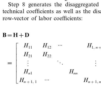
Step 8 generates the disaggregated matrix of technical coefficients as well as the disaggregated row-vector of labor coefficients:
B=H+D
=
Æ Ã Ã Ã Ã Ã È
H11 H12 ··· H1,n+1
H21 H22
· · ·
Hn1 Hnn
Hn+1, 1 ··· Hn+1,n+1
Ç Ã Ã Ã Ã Ã É
+
Æ Ã Ã Ã Ã Ã È
0 0 ··· 0 d1
d2
0 0 ··· 0 s1 s2 sn dn
−s1 −s2 ··· −sn dn+1
Ç Ã Ã Ã Ã Ã É
(14)
Blabor=Hlabor+Dlabor
=[Hlabor, 1 ··· Hlabor, n Hlabor,n+1]
+[0 ··· 0 dlabor,n+1] (15)
where the elements in H and Hlabor are obtained
according to Eq. (2) and Eq. (8), respectively. Steps 9 and 10 are necessary to obtain the matrix of inter-industry flows. Using the result of Eq. (14), the Leontief inverse is simply (I−B)−1.
If matrix B is of dimension smaller than 50×50, this inversion can be performed in simple spread-sheet packages. Consequently, the disaggregated total output column follows
BX=(I−B) −1
BY (16)
Finally, we wish to obtain the disaggregated matrix of inter-industry transactions and the row-vector of labor inputs. They satisfy the expressions
Wij=B*Bij X,j (17)
Wlabor,j=B*labor,jBX,j (18)
The results from Eq. (16) allow us to evaluate the actual changes in the total output of each other sector given the introduction of the remanu-facturing sector in the economy. Let
ri=BX,i/Xi−1
be the ratio between the total output of sector i with and without remanufacturing. It indicates the loss (or gain) in the output of that sector.
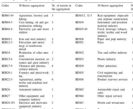
Table 2
Purchasing sector aggregation from the original 96×98 table Nr. of sectors in 30-Sector aggregation
Codes Codes 30-Sector aggregation Nr. of sectors in
the aggregation the aggregation
Agriculture, forestry and 3
BDS01-03 BDS312, 32-3 Rail equipment. shipyards 3
fishing and airplane construction
1
5 BDS34
Coal mining, oil and gas Instrument and precision BDS04-5
production, refining material industry
20 Electricity, gas and water 3 BDS35-49 Food, beverage, tobacco, BDS06-8
textile, leather and wood utilities
industry
3 BDS50
BDS09-1 Iron and steel industry Paper and pulp industry 1 Extraction and
metal-BDS12-3 2 BDS51 Press 1
lurgy of nonferrous metals
Production of other min- 1
BDS14 BDS52 Tire and rubber industry 1
erals
Construction material, ce- 2
BDS15-6 BDS53 Plastic industry 1
ramics and glass industry
BDS17-9 Chemical and pharma- 4 BDS54 Other industries 1
ceutical industry Foundry and
metal-work-BDS20-1 2 BDS55 Civil engineering and 1
construction ing
1 Agricultural, public
BDS22-5 4 BDS56 Product recovery services
works and machine tool industry
1 BDS65 Automobile repair and
Armament industry 1
BDS26
sales Office equipment and 1
BDS27 BDS66 Other repair services 1
computer industry
BDS28-291 Electrical and electronic 2 BDS67 Hotels and restaurants 1 equipment industry
Electronic home products 2 BDS68-4 Transport services
BDS292-30 7
and home appliance in-dustry
Automobile, motorcycle 1
BDS311 BDS57-64, 75-98 Other services 21
and bicycle industry
4. The impact of remanufacturing tires, computers and automobiles
Tire retreading is a healthy business in some countries, particularly in the replacement market for some industrial applications. However, its penetration in the passenger car market has re-duced steadily and represents less than 10% of the tire replacement market in most OECD countries (Ferrer, 1997b). In the French input – output tables, this business is pooled in the Tire and Rubber sector (BDS 52). Here, we ignore the market share that retreaded tires already
have, and assume that the data on the tire and rubber industry refer exclusively to new tires, to measure the likely impact of a first time intro-duction of retreaded tires.
In our 30-sector aggregation, the Tire and Rubber sector accounts for a total output of 55.69×10⁹ FF in 1991. It is the 26th largest
Comment: If the sector is split under the parameters p=0.5 and d=0.7, the total output of each sector would be around28×109 FF and
20×109 FF,respecti6ely.They would be among
the two smallest sectors in the table. Other parameter choices would ha6e similar implica
-tions. Hence, we should not expect a large impact.
It is well known that the automobile sector (BDS 311) has a great influence over the general economy, because it draws large inputs from many sectors. It includes automobiles, trucks, mo-torcycles, mopeds and bicycles.
In our 30-sector
aggregation of the French economy, 12 sectors manufacture durable goods. The total output from the automobile sector is the 5th of all sectors but the second largest among durable goods sec-tors. In fact, the automobile industry receives inputs from 23 sectors. Remanufacturing automo-biles has a strong first-order effect in most of them and significant higher-order effects in many others.
The computer manufacturing sector (BDS 27) includes portable computers, mainframes, periph-erals, and some office equipment. In this 30-sector aggregation, it receives inputs from 20 sectors. Since computer manufacturing is a very
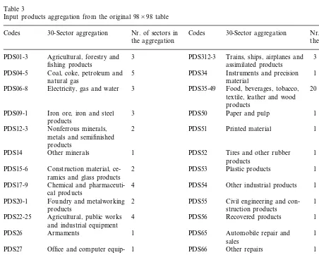
interna-Table 3
Input products aggregation from the original 98×98 table
30-Sector aggregation Nr. of sectors in Codes Nr. of Sectors in
Codes 30-Sector aggregation
the aggregation the aggregation
3 PDS312-3 Trains, ships, airplanes and
Agricultural, forestry and 3
PDS01-3
fishing products assimilated products
5 PDS34 Instruments and precision Coal, coke, petroleum and
PDS04-5 1
material natural gas
Food, beverages, tobacco, PDS35-49
3 20
Electricity, gas and water PDS06-8
textile, leather and wood products
PDS09-1 Iron ore, iron and steel 3 PDS50 Paper and pulp 1 products
PDS51
2 1
Nonferrous minerals, Printed material
PDS12-3
metals and semifinished products
Other minerals 1
PDS14 PDS52 Tires and other rubber 1
products Plastic products PDS53
2 1
PDS15-6 Construction material, ce-ramics and glass products
Chemical and pharmaceuti- 1
PDS17-9 4 PDS54 Other industrial products
cal products
1 PDS20-1 Foundry and metalworking 2 PDS55 Civil engineering and
con-products struction products
Agricultural, public works 4 PDS56 Recovered products 1 PDS22-25
and industrial equipment
Armaments 1
PDS26 PDS65 Automobile repair and 1
sales
1 Office and computer equip- Other repairs
PDS27 1 PDS66
ment
Hotels and restaurants PDS67
2 Electrical and electronic
PDS28, 291 1
equipment
PDS292, 30 Electronic home products 2 PDS68-4 Transport services 7 and home appliances
tional business, most computers actually con-sumed in France are manufactured abroad. For this reason, it is just the 23rd largest sector in this aggregation, the 7th among the 12 sectors that manufacture durable goods. However, since the input – output table only refers to the inter-indus-try transactions occurring within a region — in this case, France — an eventual remanufacturing industry is likely to process (or produce) more units than were originally manufactured within the country. We do not deal with this possibility now. One could treat this phenomenon by including the Import sector in the analysis. This would account for the substitution of some inputs from this source by the remanufactured units produced in the country.
For the sake of simplicity, we assume that the market absorbs all of the output from the reman-ufacturing sectors. Producers of recycled paper know that this is not always true. The stochastic aspects of input availability and demand for out-puts have a significant influence over the econom-ics of any product recovery activity. However, since our interest is in understanding the impact of successful remanufacturing sectors, we believe that we can concentrate in the basic model, without uncertainty.
4.1. Parameter choices
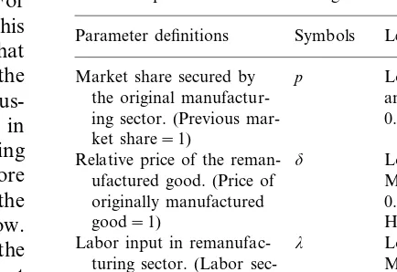
In what follows we disaggregate the 30×30 input – output table of the French economy to examine the impact of remanufacturing tires, com-puters and automobiles. The individual impacts are driven by the parameters defining the respec-tive distinguishing matrix. Hence, we examine a number of scenarios, corresponding to different levels of market share, and different levels of price discount offered by the remanufactured products. Table 4 describes these scenarios. In all scenarios, the following assumptions are observed.
1. The final demand for the product (in physical units) is not changed and the remanufactured product is sold at a lower price. Or, q=
d*(1−p). (This is a very conservative assump-tion, because if price elasticity is negative, as with most products, sales in physical units is sure to increase.)
Table 4
Economic parameters for evaluating remanufacturing effects Parameter definitions Symbols Levels
p
Market share secured by Low (p=0.4) the original manufactur- and high (p= ing sector. (Previous mar- 0.6)
ket share=1)
Low (d=0.5)
d
Relative price of the
reman-ufactured good. (Price of Medium (d= originally manufactured 0.6)
good=1) High (d=0.7)
Low (l=1.2)
l
Labor input in
remanufac-Medium (l= turing sector. (Labor
sec-1.5) tor input in original
High (l=1.8) manufacturing=1)
2. Since remanufactured items cost less, and the physical demand from both sectors remains the same, an additional income becomes avail-able and is re-spent in the form of additional demand to all sectors. See Eq. (10).
3. The increased demand for labor and trans-portation compensates the decreased demand for raw materials and energy. See Eq. (12). If the market share secured by the original manufacturing sector since the introduction of remanufacturing is p, then the final demand for the products from the original manufacturing sec-tor is multiplied by p. Moreover, in the aug-mented matrix, the row corresponding to the inputs from original manufacturing to all other sectors has all elements multiplied by the same factor p. (Subsequently, the augmented technical coefficients are adjusted by the parameters sj in
the distinguishing matrix, as described in the pre-vious section.)
remanufacturing becomes a significant competitor of the original manufacturing sector. They were chosen as follows:
Market shares of 40 and 60% correspond to situations where both the remanufacturing and original manufacturing sectors hold significant participation in the economy. Values smaller than 40% are not reasonable: it would imply that the original manufacturing sector would gradually disappear. Values above that would not satisfy the problem’s original condition that remanufacturing gains a significant share of the market.
A value of d=0.7 implies that the remanufac-tured good is sold for a 30% discount over the price of the originally manufactured good. In France, remanufactured photocopiers are sold for roughly 40% discount over the price of new photocopiers of the same manufacturer (d=
0.6). The additional scenarios with d=0.5 (high discount) and d=0.7 (low discount) cover a reasonable neighborhood of the ob-served value.
The ratio between the direct labor intensity in each industry is bound by practical limitations. It cannot be lower than 1.0 (since it would imply that remanufacturing is less labor inten-sive than original manufacturing). These tables show that in these sectors labor inputs range from 22% (in the automobile sector) to 42% of total inputs (in the tire sector). In order to allow the remanufacturing and the original manufacturing sectors to have the same profitability, the direct labor intensity ratio cannot be greater than roughly 2.3. Labor in-creases as a substitution of inputs that are not needed in remanufacturing, but not all inputs can be substituted. This constitutes a practical upper bound of roughly 2.0 for the direct labor intensity ratio. We usel=1.2 (low estimate for labor substitution), l=1.5 (medium) and l=
1.8 (high) which seem to be good representa-tives of the feasible range (1.0 – 2.0).
Obviously remanufacturing is inherently much less able to capture large scale advantages of standardized mass production than primary man-ufacturing. A remanufacturing operation neces-sarily deals with a number of different models and
ages, each of which involves different setups and tools. The heterogeneous input stream must clearly be sorted into lots before further opera-tions are undertaken, and since very small lots are uneconomic, a significant amount of storage space may be needed as lots accumulate to critical size. However, as remanufacturing becomes more the rule than the exception, production runs will in-crease. Developments in computer-integrated manufacturing and programmable automation have reduced the disadvantage of small lots, and this trend can be expected to continue. Finally, successive models can be designed to minimize differences in disassembly, setup and processing costs. Thus, the scale-related penalty of remanu-facturing is expected to reduce in the course of time.
Most of these added costs (of processing small lots) are labor costs. Thus, as remanufacturing increases, direct employment increases. Clearly, these added costs impose a limit on the economic feasibility of remanufacturing. Although environ-mental benefits may be significant, the primary concern for a firm must be its own cost structure. It can justify remanufacturing only if other cost reductions compensate for the higher labor requirements.
Overall, we have limited our analysis to three levels of labor cost increase, ranging from low (l=1.2) to high (l=1.8). It means that, if the labor increase in the remanufacturing sector is l, then each monetary unit of output from this sector requires labor inputs equivalent to those required by the original manufacturing sector multiplied by l. Since the inputs from the Trans-port Services sector are also increased, and the total inputs from all sectors are the same as in the original manufacturing sector, there will be a sub-stantial decrease in some of the other inputs. (This trade-off characterizes the remanufacturing pro-cess, where physical inputs such as raw materials or semi-finished goods are traded against labor time in recovering the used goods.)
Venta and Wolsky (1978) have examined the aggregate demand for labor and energy in the automobile component remanufacturing sector. There, the purpose is to obtain a measure of total energy and labor consumed by the sector. This work differs from their analysis because it is a comparison between two economies (with and without remanufacturing). However, it provides some guidance in terms of the sectors directly affected by automobile component remanufactur-ing, as well as the magnitude of these effects. In addition, Das et al. (1995) provides information regarding the type and quantity of raw materials
and the amount of energy required in automobile production. Studies by Ferrer (1997a,b) analyzed the economics of remanufacturing tires and per-sonal computers, respectively. Information from these studies was useful in estimating the input requirements of hypothetical remanufacturing sectors.
A complete disaggregation requires estimating the parameters that distinguish the sectors accord-ing to the technology used (dj) and the parameters
that distinguish them according to their markets (sj). Unfortunately, we have little information
available that could be useful in determining the
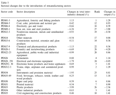
Table 5
Sectoral changes due to the introduction of remanufacturing sectors
Changes in total inter- Rank Changes in total Rank Sector code Sector description
industry demand (%) output (%)
1 1.29 6
1.13 PDS01-3 Agricultural, forestry and fishing products
0.42 12 0.93
PDS04-5 Coal, coke, petroleum and natural gas 11
19 0.39
18 −0.66
PDS06-8 Electricity, gas and water
−6.28 27 −3.90 27 PDS09-1 Iron ore, iron and steel products
−0.30 24 19
PDS12-3 Nonferrous minerals, metals and semifinished −0.93 products
17 0.04
PDS14 Other minerals −0.54 22
20 0.36
14 PDS15-6 Construction material, ceramics and glass 0.11
products
22 0.36
PDS17-9 Chemical and pharmaceutical products −1.13 21
28 −4.20
PDS20-1 Foundry and metalworking products −6.69 28
13
20 0.86
PDS22-25 Agricultural, public works and industrial −0.99 equipment
0.80 4 1.14
PDS26 Armaments 8
23 −0.05
24 −1.79
PDS28, 291 Electrical and electronic equipment
0.69 5 1.41 1
PDS292, 30 Electronic home products and home appliances
1.29 5
2 PDS312-3 Trains, ships, airplanes and assimilated prod- 0.99
ucts
25 0.81
PDS34 Instruments and precision material −1.95 16
7 1.18
13 PDS35-49 Food, beverages, tobacco, textile, leather and 0.25
wood products
6 0.86
PDS50 Paper and pulp 0.59 14
7 0.90
PDS51 Printed material 0.54 12
−2.36
26 26
−3.99 PDS53 Plastic products
0.83 3 1.41
PDS54 Other industrial products 3
1.41 2
PDS55 Civil engineering and construction products 0.48 10
23 −1.47
PDS56 Recovered products −1.48 25
15 1.02 9
−0.05 PDS65 Automobile repair and sales
0.93 10
PDS66 Other repairs −1.10 21
4 1.35
8 0.51
PDS67 Hotels and restaurants
0.84 15
PDS68-4 Transport services 0.47 11
0.74 17
PDS75-98 Other services −0.26 16
9 0.49
market deviation parameters. Ideally, remanufac-tured products have as good a performance as originally manufactured products. Hence, if they cost less, ‘utilitarian’ sectors would rather buy from the remanufactured sector than from the original manufacturing sector, if available. For example, tires purchased by the agricultural sector would come from the tire retreading industry, rather than from the new tires industry. On the other hand, if the good is a direct input of an original product (e.g. tires as a production input in automobile manufacturing), that sector will only buy the original version. We used that logic as the basis for estimating the market deviation parameters.
4.2. The impact of de6eloping remanufacturing
sectors
In this analysis, we disaggregate a 30-sector table to introduce three new sectors: Computer Remanufacturing, Automobile Remanufacturing and Tire Retreading. Table 4 suggested evaluating two different levels of market share, three levels of price discount and three levels of labor require-ments. Considering the French economy in 1991 as an appropriate benchmark, we evaluated all 18 possible scenarios derived from the table of parameters.
The development of the remanufacturing sec-tors causes the changes in the output of the other sectors. Table 5 shows the impact in the scenario where there is medium labor increase (l=1.5), medium market share (p=0.5), high discount on remanufactured goods (d=0.5). The table shows two columns of changes. The sectors that lose most inter-industry transactions are the ones providing raw materials and components to the
three sectors analyzed: foundry and metal-work-ing (PDS20-1), iron and steel products (PDS09-1), plastic products (PDS53) and electric and elec-tronic products (PDS28, 291). They are also the sectors with greatest reduction in total output.
In addition, Table 6 shows that each original sector suffered different changes in inter-industry and total output. In this scenario, the final de-mand for each of the original manufacturing sec-tors was reduced by 50% (p=0.5). Other things equal, one might expect that their inter-industry transactions observe changes of the same magni-tude. However, each sector experienced a different reaction. Reduction in the inter-industry transac-tions of the tire industry was closer to 56% (larger than 50%). It happens that the tire industry de-pends largely on its transactions with the automo-bile industry. That greater reduction in the transactions of the tire industry is caused by a large second-order effect from the automobile in-dustry. Contrariwise, the automobile and the computer industries observed a reduction in their inter-industry transactions of 41 and 46%, respec-tively. They depend very little on the transactions with the other industries where we created a re-manufacturing dual. Hence, the second-order ef-fects are not as significant. Moreover, all three original manufacturing sectors become large sup-pliers of their respective remanufacturing sectors, as the main source of components, dampening the reduction of their final demand.
One of our concerns was the impact of remanu-facturing in the demand for labor. There is a persistent argument whether remanufacturing ac-tivities have positive or negative impact on de-mand for labor. Although remanufacturing per se is labor intensive, it reduces the need for several outputs that are labor intensive as well. Table 7
Table 6
Sectoral changes due to the introduction of remanufacturing sectors (cont’d)
Changes in total Changes in total inter-industry
Original manufacturing sector Sector code
demand (%) demand (%)
description
Automobiles, motorcycles and bicycles −40.7 −47.8 PDS311
−45.5 −48.3 PDS27 Office and computer equipment
Tires and other rubber products −55.8
Table 7
Changes in total labor output under different economic scenarios
Market share of original product Low (P=0.4) High (P=0.6)
Low Medium High Low
Labor increase in remanufacturing Medium High
(l=1.2)
(l=1.5) (l=1.8) (l=1.5)
(l=1.2) (l=1.8) sector
Low (d=0.5) 0.56% 0.69% 0.82% 0.35%
Price of the reman- 0.44% 0.52%
Medium (d=0.6) 0.45% 0.60%
ufactured 0.75% 0.28% 0.38% 0.48%
product High (d=0.7) 0.34% 0.51% 0.69% 0.21% 0.33% 0.45%
shows the changes in labor output under 18 sce-narios. Each scenario required more labor, rang-ing from 0.21 to 0.82% increase in labor output. We derived the following linear regression model relating the changes in labor with economic parameters:
%Labor change=(0.83+0.42*l−1.08*p
−0.71*d)%
Example: in the scenario where l=1.5, p=0.5
and d=0.5,the formula indicates that demand for labor would increase by 0.494%. Calculations dis -aggregating the original input–output tables would suggest an increase of 0.489%.
The greatest labor increases occur when the remanufacturing sector has large market share and requires more labor (at the expense of inputs from many other sectors). Moreover, labor output increases with the price discounts adopted by the remanufacturing sector. This implies that
remanu-facturing provides more direct and indirect labor than original manufacturing.
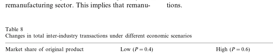
Finally, there is a concern whether remanufac-turing operations promote growth or not. Table 8 sheds the light over this issue. By construction, we had imposed that the sum of final demands from all sectors remained constant. This was accom-plished by distributing the income saved with the purchase from the remanufacturing sector among all sectors (as explained in the previous section). However, as we let the inter-industry transactions accommodate the new economic structure, we observe a generalized reduction of inter-industry activity, ranging from−0.32 to−0.75%. It is a point of debate whether this reduction is ‘healthy’ for the economy or not. One may argue that for a fixed level of final demand, fewer inter-industry transactions imply in a more efficient economy. If that argument is correct, we might say that a remanufacturing economy is more efficient, even before we consider the environmental implica-tions.
Table 8
Changes in total inter-industry transactions under different economic scenarios
Low (P=0.4) High (P=0.6) Market share of original product
High Low High
Labor increase in remanufacturing Low Medium Medium
sector (l=1.2) (l=1.5) (l=1.8) (l=1.2) (l=1.5) (l=1.8) −0.54% −0.47%
Price of the reman- Low (d=0.5) −0.54% −0.65% −0.75% −0.40% −0.63%
ufactured Medium (d=0.6) −0.51% −0.76% −0.37% −0.45% −0.53%
−0.75% −0.32% −0.42% −0.52% High (d=0.7)
5. Conclusion
The purpose of this study is 3-fold: to develop a methodology for disaggregating the input – out-put tables to incorporate remanufacturing sectors as competitors of existing manufacturing sectors; to illustrate the methodology using a 30×30 ver-sion of the input – output tables for the French economy in 1991; to identify the direction of changes in the demand for labor and in the total inter-industry transactions given the development of remanufacturing sectors.
The methodology is simple, requiring the esti-mation of 2n+2 parameters for each remanufac-turing sector introduced in the table. They regard the difference in the technology used by the re-manufacturing sector (n+1 parameters), the dif-ferent purchasing preferences that each sector has regarding the remanufactured product (n parame-ters) and the different need for labor (one parameter). For the illustration, we estimated some parameters based on previous studies. How-ever, market-related parameters could not be eval-uated very precisely. Their estimation was based on the most-likely buying behavior of the other sectors. (Further research is required in that do-main.) Finally, the analysis of the French econ-omy led to the following observations:
1. Remanufacturing activity promotes demand for labor.
2. Remanufacturing activity reduces the level of inter-industry transaction.
3. Suppliers of sectors subject to competition from remanufacturing sectors have their inter-industry transaction significantly reduced. That situation is exacerbated if the sector is also subject to remanufacturing activity.
Acknowledgements
The authors would like to thank Landis Gabel, Faye Duchin and two anonymous referees for
their valuable comments that allowed for signifi-cant improvements in this paper.
References
Ayres, R.U., Ferrer, G., Van Leynseele, T., 1997. Eco-effi-ciency, asset recovery and remanufacturing. Eur. Manag. J. 15 (5), 557 – 574.
Das, S., Curlee, T.R., Rizy, C.G., Schexnayder, S.M., 1995. Automobile recycling in the United States: energy impacts and waste generation. Resources Conserv. Recyc. 14, 265 – 284.
Davis, H.C., 1987. Accounting for technical substitution in the input – output model. Technol. Forecasting Soc. Change 32 (4), 361 – 371.
Driver, C., 1994. Structural change in the UK 1974 – 1984: an input output analysis. Appl. Econ. 26 (2), 153 – 158. Feldman, S.J., McClain, D., Palmer, K., 1987. Sources of
structural changes in the United States, 1963 – 78: an in-put – outin-put perspective. Rev. Econ. Stat. 69 (3), 503 – 510. Ferrer, G., 1997a. The economics of personal computer re-manufacturing. Resources Conserv. Recycl. 21, 79 – 108. Ferrer, G., 1997b. The economics of tire remanufacturing.
Resources Conserv. Recycl. 19, 221 – 255.
Hannan, M.J., Rose, A.Z., 1988. The policy-cost index ap-proach to modeling change in input – output coefficients: an application to acid rain policy. Technol. Forecasting Soc. Change 33 (1), 13 – 22.
Howell, D.R., 1985. The future employment impacts of indus-trial robots: an input – output approach. Technol. Forecast-ing Soc. Change 28 (4), 297 – 310.
INSEE, 1995. Les Tableaux des Entre´es et Sorties. Paris, France, INSEE.
Lee, K.-S., 1982. A generalized input – output model of an economy with environmental protection. Rev. Econ. Stat. 64, 466 – 473.
Leontief, W., 1936. Quantitative input – output relations in the economic system of the United States. Rev. Econ. Stat. 18 (3), 105 – 125.
Lowe, P.D., 1979. Pricing problems in an input – output ap-proach to environmental protection. Rev. Econ. Stat. 61 (1), 110 – 117.
Rhee, J.J., Miranowski, J.A., 1984. Determination of income, production, and employment under pollution control: an input – output approach. Rev. Econ. Stat. 66 (1), 146 – 150. Venta, E.R., Wolsky, A.M. 1978. Energy and Labor Cost for Gasoline Engine Remanufacturing. Argonne National Laboratory. September 1978. Argonne, IL.
Wolsky, A.M., 1984. Disaggregating input – output models. Rev. Econ. Stat. 66 (2), 283 – 291.
.