Vol. 43 (2000) 239–262
Spatial evolution of automata in the prisoners’
dilemma
Oliver Kirchkamp
1University of Mannheim, SFB 504, L 13, 15, D-68131 Mannheim, Germany
Received 17 October 1996; received in revised form 9 February 2000; accepted 8 March 2000
Abstract
We apply the idea of evolution to a spatial model. Prisoners’ dilemmas or coordination games are played repeatedly within neighbourhoods where players do not optimise but instead copy suc-cessful strategies. Discriminative behaviour of players is introduced representing strategies as small automata, which can be in different states against different neighbours. Extensive simulations show that cooperation persists even in a stochastic environment, that players do not always coordinate on risk dominant equilibria in 2×2 coordination games, and that success among surviving strate-gies may differ. We present two analytical models that help understanding of these phenomena. © 2000 Elsevier Science B.V. All rights reserved.
JEL classification:C63; C73; D62; D83; R12; R13
Keywords:Evolutionary game theory; Networks; Prisoners’ dilemma; Coordination games; Overlapping generations
1. Introduction
Evolutionary models have in the last years become increasingly popular to study spatial phenomena. These models frequently concentrate on prisoners’ dilemmas and coordination games and often share the following assumptions: Players may not discriminate among neighbours, have small memory and interact and learn synchronously. As we will see in the following, the impact of these assumptions may be crucial.
We use a spatial model to describe a world where agents interact with each other to different degrees. An example of a spatial prisoners’ dilemma is firms located in space and competing for customers who are placed among these firms. Firms could set high prices,
∗E-mail address:[email protected] (O. Kirchkamp).
1http://www.kirchkamp.de/
aiming at a monopoly profit if neighbouring firms set high prices as well. Firms could also set low prices hoping to undercut prices of other firms and, thus, stimulating demand for their own product.2
In a world without space the above example is a trivial case of Bertrand competition. In a spatial world where all firms do not share the same market, the problem is less trivial, since Hotelling (1929) a lot of spatial models have been specified and solved. Most of these models assume perfect rationality. We, however, study a simple evolutionary process. Strategies grow as long as they are successful, unsuccessful strategies vanish from the population.3 This dynamics has a biological and a social interpretation. Biologically it models a birth process where successful strategies produce more offspring and a death process where unsuccessful strategies are more likely to die soon. In social contexts we assume successful strategies more likely to be copied while unsuccessful strategies are more likely to be abandoned. The evolutionary dynamics will be applied in a spatial context — immobile agents play games with their neighbours and imitate successful neighbours’ strategies.
One of the issues we will discuss is the timing of interaction and learning in these models. Most of the literature4 assumes interaction and learning to be synchronised. We will compare this case with random and asynchronous learning and interaction. Another issue that we will discuss is memory of players and their ability to react or to discriminate. The literature5 usually assumes that players may not react on their opponent’s past actions and may not distinguish among their neighbours. We will investigate the impact of this assumption, modelling player’s strategies as small automata.
As a result, we find that a common property of non-spatial evolutionary models, equal payoffs of surviving strategies, vanishes in space when players may discriminate among their neighbours. We present simulation results and give a motivation with a simplified discrete model which can be solved analytically. We compare simulation results with a simple continuous model which reliably approximates the discrete model both for prisoner’s dilemmas and for coordination games. We identify and study parameters that determine the choice of strategies in prisoners’ dilemmas and coordination games. We find that players choose equilibria in coordination games following a criterion that is between risk dominance and Pareto dominance.
We will study a model where a network structure is given, where players are immobile and learn through imitation. Let us briefly mention some related models that take different approaches.
A model where the network structure emerges endogenously is studied by Ashlock et al. (1994), who allow players to ‘refuse to play’ with undesired opponents. Their model presupposes no spatial structure ex ante — determining the structure endogenously is one way to allow for discriminative behaviour. In our model we take a different approach: The
2An example for a spatial coordination game can be found similarly: Neighbouring firms could be interested in
finding common standards, meeting in the same market etc.
3See, e.g. Maynard Smith and Price (1973) for static concepts and Taylor and Jonker (1978) and Zeeman (1981)
for a dynamic model.
interaction structure is fixed and strategies are small automata which also allow players to treat different opponents differently.
Models where players are mobile are introduced by Sakoda (1971) and Schelling (1971) as well as by Hegselmann (1994). These models assume that some properties of an agent (e.g. colour of skin as in Sakoda or a risk-class as in Hegselmann) are invariably fixed but that agents can move. These models offer an explanation for segregation of a population into patches of agents with different types.
Ellison (1993) studies a model where players play coordination games against their neighbours and optimise myopically. As a result these players quickly coordinate on the risk-dominant equilibrium. We will see in Section 5.4 below that myopic imitation may choose a different equilibrium.
The assumptions of a given network structure, immobile players and learning through im-itation are shared by Axelrod (1984, p. 158ff.), May and Nowak (1992, 1993), Bonhoeffer et al. (1993), Lindgreen and Nordahl (1994) and Eshel et al. (1998). What is different in our ap-proach is the introduction of discriminative strategies together with asynchronous behaviour. Axelrod (1984, p. 158ff.) analyses a cellular automaton where all cells are occupied by players that are equipped with different strategies. Players obtain each period payoffs from a tournament (which consists of 200 repetitions of the underlying stage game) against all their neighbours. Between tournaments, players copy successful strategies from their neighbourhood. This process gives rise to complex patterns of different strategies. Axelrod finds that most of the surviving strategies are strategies that are also successful with global evolution. Nevertheless some of the locally surviving strategies show only intermediate success in Axelrod’s global model. These are strategies that get along well with themselves but are only moderately successful against others. They can be successful in the spatial model because they typically form clusters where they only play against themselves.
A similar model has been studied by Lindgreen and Nordahl (1994), who in contrast to Axelrod do not analyse evolution of a set of pre-specified strategies, but instead allow strategies to mutate and, hence, allow for a larger number of potential strategies. Similar to Axelrod, Lindgren and Nordahl assume that reproductive success of a strategy is determined by the average payoff of an infinite repetition of a given game against a player’s neighbours. While Axelrod and Lindgren and Nordahl study a population with a large number of pos-sible strategies, May and Nowak (1992) analyse a population playing a prisoners’ dilemma where players can behave either cooperatively or non-cooperatively. They study various ini-tial configurations and analyse the patterns of behaviour that evolve with synchronous inter-action. Bonhoeffer et al. (1993) consider several modifications of this model: They compare various learning rules, discrete versus continuous time and various geometries of interaction. Eshel et al. (1998) derive analytically the behaviour of a particular cellular automaton. The price they have to pay for the beauty of the analytical result is the restriction to a small set of parameters. They have to assume a particular topology and neighbourhood structure. They find that there is a range of prisoners’ dilemmas where increasing the gains from cooperation reduces the amount of players who actually cooperate. It is not clear how their result depends on the particular set of parameters they analyse.
discrimi-native behaviour might seem similar to the repeated game strategies used by Axelrod and by Lindgren and Nordahl. However, there is an important difference. Most of the litera-ture, including Axelrod and also Lindgren and Nordahl, assumes that updates of players’ strategies as well as players’ interactions occur synchronously. As we shall see below such a synchronisation has substantial impact on the evolutionary dynamics. In a biological ap-plication synchronisation is naturally motivated through seasonal reproduction patterns. In social or economic contexts synchronisations are harder to justify. We, therefore, introduce discriminative strategies without requiring synchronisation.
That introducing asynchronous interaction and evolution might matter has also been men-tioned by Huberman and Glance (1993), who argue that cooperation might be extinguished through introduction of asynchronous behaviour. Bonhoeffer et al. (1993), however, argue that introducing asynchronous behaviour matters only little. As will be seen in the follow-ing not the mere fact of introducfollow-ing asynchronous behaviour determines the amount of cooperation. It is the way how asynchronous behaviour is introduced that determines the persistence or breakdown of cooperation.
While the cellular automaton model of a population and the introduction of discrimi-native behaviour incorporates more real life flavour, it is on the other hand more difficult to analyse. We replace analytical beauty by extensive simulations. We carried out about 60 000 simulations on tori ranging from 80×80 up to 160×160 and continuing from 1000 to 1 000 000 periods. We find that most of the results vary only slightly and in an intuitive way with the parameterisation of the model.
Section 2 describes a continuous model that can be solved analytically and that explains growth of strategies in a spatial but continuous world. The spatial model will be presented in Section 3. In Section 4, we start with a simplified version, a discrete model that exem-plifies permanent exploitation among strategies — a property that is important for spatial evolution. Simulation results will be presented in Section 5. Section 5.2 connects our re-sults to the findings of May and Nowak (1992, 1993) by comparing several models with non-discriminative strategies. Section 5.3 introduces discriminative behaviour, Section 5.4 extends the analysis to coordination games and Sections 5.5 and 5.6 discuss robustness of the results. Section 6 finally draws some conclusions.
2. A continuous model
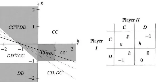
In the following we concentrate on symmetric 2×2 games and in particular on prisoners’ dilemmas. Stage game strategies are named C and D. We represent the space of all symmetric prisoners’ dilemmas with the game shown in Fig. 1.6 To make the interpretation of the results presented in Section 5 below easier, we will start with a continuous model that aims to explain growth of clusters of strategies.
We will first study a model where patches of homogeneous strategies, that we will call ‘clusters’, are relatively large. We will then extend this model to capture smaller clusters too.
6All the dynamics of population behaviour that are discussed in the following are invariant to transformations
Fig. 1. The parameterisation of the underlying prisoners’ dilemma game. The game is a prisoners’ dilemma for 0< g <1, h <0 andg >12+
1
2h. We requireg <1 andh <0 to ensure that C is a dominated strategy of the
stage game. Then 0< gandg >12+12hmake certain that CC Pareto dominates both DD and cycling between CD and DC.
We assume that players are continuously distributed along a line and interact and learn within a radiusr. Players play the game described in Fig. 1 and copy the strategy with the highest average payoff in their learning neighbourhood. Let us first assume that the world consists of only two clusters that are both larger than 2r.
Let us consider a player at positionxˆbetween two of these clusters. All players at position x <xˆplay C, all players atx >xˆplay D. A player that lives at positionxmeets another can be calculated for the player atxˆas
uC(x)ˆ = 14(3g+h), uD(x)ˆ = 14 (2)
A player at positionxˆwill imitate a C ifg > 13(1−h)and a D ifg < 13(1−h). In either case clusters will grow until one strategy disappears completely.
In the above paragraph we have studied a world where strategies were allocated in two big clusters each. In the following we will assume the world consists of a sequence of alternating clusters of Cs and Ds. The C playing clusters have radiusnCr, wherenC∈[1,2] and the D playing clusters have radiusnDr, wherenD∈[1,2].7 A player who lives precisely between two clusters sees for both clusters a proportion of
F (n)=14(5−4n+n2) (3)
(forn=nCandn=nD) playing against the respective opposite strategy. The remaining 1−F (n)play against their fellows which are in the same cluster. Average payoffs are
uC(x)ˆ =(1−F (nC))g+F (nC)h, uD(x)ˆ =F (nD) (4)
7The precise analysis of even smaller clusters becomes really tedious. We think that it is reasonable to assume
The differenceuC(x)ˆ −uD(x)ˆ is a quadratic function ofnCandnD:
Similar to Eq. (2) also inequality (6) gives us a condition that determines when clusters of C or D grow, shrink or remain stable. We will use these conditions below to represent our results.
In the following we will move to a discrete model that will be described in Section 3. Players are of discrete size, we will most of the time consider a two dimensional network and the size of the clusters is determined endogenously. We will see that the continuous model of the current section gives a fairly good approximation of the properties of the discrete model that we will study in the following.
3. A discrete spatial model
3.1. Space and time
Players are assumed to live on a torus.8The torus is represented as a rectangular network, e.g. a huge checkerboard. The edges of this network are pasted together. Each cell on the network is occupied by one player. Using a torus instead of a plain checkerboard avoids boundary effects. Most simulations were carried out on a two-dimensional torus of size 80×80. The results presented in Sections 5.5 and 5.6 show that neither the exact size of the network nor the dimension matters significantly.
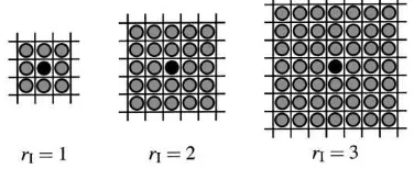
In contrast to models of global evolution and interaction we assume players to interact only with their neighbours and learn only from their neighbours. Each player has an ‘interaction neighbourhood’ of radiusrIas shown in Fig. 2 which determines the set of the player’s possible opponents. In the same way we construct a ‘learning neighbourhood’ with a similar structure, but with a possibly different radiusrL. Each player observes payoffs and strategies within the learning neighbourhood.
We will compare synchronous with asynchronous interaction and learning. With syn-chronous interaction players interact in each period with all their neighbours. With asyn-chronous interaction a random draw decides in each period for each pair of neighbours
8In Section 5.6 we investigate some other topologies where players are located on a circle, on a cube, or on a
Fig. 2. Neighbourhoods with interaction radius 1, 2 and 3. Possible interaction partners of a player are described as grey circles while the player itself is represented as a black circle.
whether the mutual interaction takes place. Hence, with asynchronous interaction in differ-ent periods the composition of oppondiffer-ents may be differdiffer-ent. With synchronous learning all members of a population will learn simultaneously everytLperiods. With asynchronous learning, each strategy has an individual random ‘lifetime’tL. As soon as the lifetime of the strategy expires, the individual player learns and possibly adopts a new strategy with again a random lifetime which may differ from the previous one.
3.2. Strategies
Strategies may be discriminative or non-discriminative, i.e. players may or may not be able to treat different neighbours differently. With non-discriminative strategies players either play C against all neighbours or they play D against all of them. Discriminative strategies are modelled as Moore automata with less than three states.9We have done several simulations with more complex automata and found that results do not change much when the number of states is increased to three or four.
3.3. Relevant history for learning
To choose a strategy players have to learn. To do that they use information available in their neighbourhood: Their neighbours’ average payoffs (per interaction) and their strategies. We compare two extreme cases: Learning players may consider only today’s payoffs when calculating average success of a neighbour’s strategy or learning players consider payoffs from all periods while the neighbour used the same strategy as today. The first case will be called ‘short memory’ and the second ‘long memory’.
9Each ‘state’ of a Moore automaton is described with the help of a stage game strategy (C or D) and a transition
3.4. Learning
We will compare two learning rules. Both are based on the assumption that players are not fully rational, they are not able or not willing to analyse games, and they do not try to predict their opponents’ behaviour. Instead, behaviour is guided by imitation of successful strate-gies. ‘Copy best player’ copies the strategy of the most successful player in the neighbour-hood.10 ‘Copy best strategy’, instead, copies the strategy that is on average (per interaction) most successful in the neighbourhood.11 Players that continue to use their old strategy af-ter learning took place continue to use it in which states it currently is against the different neighbours. Players that learn a new strategy start using this strategy in the initial state.
3.5. Initial state of the population
The network is initialised randomly. First relative frequencies of the available strategies are determined randomly (following an equal distribution over the simplex of relative fre-quencies) and then for each location in the network an initial strategy is selected according to the above relative frequencies of strategies. Hence, simulations start from very different initial configurations.
4. A simple discrete model with only two strategies
Before we start presenting simulation results let us first discuss a simpler model that allows us to understand an interesting property of the discrete model, mutual exploitation. For the simplified model that we discuss in this section we make the following assump-tions:
1. There are only two strategies present in the population: Grim and blinker. Grim is a strategy that starts with C and continues to play C unless the opponent plays at least one D. From then on grim will play D forever. Blinker alternates between C and D all the time.
2. Players interact with each of their opponents in each period exactly once.
3. Players do not observe their neighbours’ payoffs but average payoffs of strategies over the whole population. They use the ‘copy best strategy’ learning rule, i.e. when they learn they copy the strategy with the highest average payoff (per interaction) in the population. 4. Players will learn very rarely. The individual learning probability in each period isǫ.
We assume thatǫ→0.
The most crucial departure from our simulation model is assumption 3: Learning is based on average payoffs of the whole population and not of the individual neighbourhood. This simplifies the analysis substantially. Simulations below show that the assumption is harmless.
10If more than one player has highest average payoff, a random player is picked, unless the learning player is
already one of the ‘best players’. In this case the learning player’s strategy remains unchanged.
11If more than one strategy has highest average payoff, a random strategy is picked, unless the learning player
We will denote possible states of grim withGC andGD, depending on whether grim is in its cooperative or its non-cooperative state. Similarly we denote possible states of blinker withBCorBD. The average payoff per interaction of grim and blinker in a given period is denoted withu¯G andu¯B. In the following we will describe an evolutionary
dy-namics of a population that has a cyclical structure. We define a cyclical equilibrium as follows:
Definition 1(Cyclical equilibrium). A cyclical equilibrium is a sequence of states of a population that, once such a sequence is reached, it repeats forever.
In the model that we consider below, all of our cycles have length one or two. We will not only consider cycles of complete states of the population, but also cycles of average payoffs or cycles of relative frequencies of strategies or pairs of strategies. We will denote a cycle of any two objectsaandbwith the symbol⌈ab⌉. When we mention several cycles in the same context, like⌈ab⌉and⌈cd⌉, then we want to say thata happens in the same period as cwhile b happens together with d. A cycle of length one can be denoted as
⌈a⌉. When we mention⌈a⌉together with⌈bc⌉we want to say that a population alternates between a state whereahappens together withband another state whereahappens together withc.
Proposition 1. Under the above assumptions there are four possible classes of cyclical equilibria.
1. A population that contains any proportion of⌈hGC, GCi⌉and⌈hGD, GDi⌉is in a cyclical
equilibrium.
2. A population that contains any proportion of the cycles of pairs⌈hBC, BCihBD, BDi⌉,
⌈hBD, BDihBC, BCi⌉and⌈hBC, BDi⌉is in a cyclical equilibrium.
3. There are cyclical equilibria where in both periods average payoffs of grim and blinker are equal.
4. There is a single cyclical equilibrium where both grim and blinker are present and have different payoffs at least in some periods.This equilibrium has the property that payoffs alternate betweenu¯G = 12ǫ(1+2h) <u¯B = 12ǫandu¯G = 12 >u¯B = 12(g+h).12
One-fourth of the population consists of pairs⌈hGD, GDi⌉,half of the population consists
of a cycle of pairs⌈hGD, BDihGD, BCi⌉and one-fourth of the population consists of a
cycle of pairs⌈hBD, BDihBC, BCi⌉. The proof is given in Appendix A.
The interesting case is case 4. It shows how one strategy earns substantially less than average payoff but still does not die out. Both strategies replicate in exactly the same number of periods and at the same speed alternating in having more than average pay-off. For reproductive success it does not matter that one of the two strategies is only an ǫ more successful when it replicates, while the other replicates with a substantial payoff difference. We will come back to this argument in the discussion of Fig. 8.
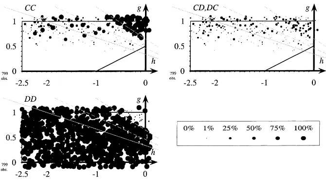
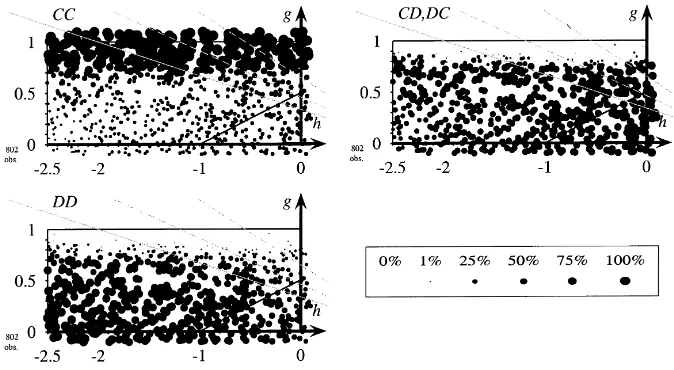
Fig. 3. Frequency of CC, CD, and DD with non-discriminative strategies. Non-discriminative strategies,pI=1,
tL=1, copy-best-player, short memory,rL=rI=1, network=80×80.
5. Simulation results
5.1. Representation of the results
To explain the representation of the results let us look at Fig. 3. The figure shows the results of 800 different simulations, each for a different (randomly chosen) game, and each lasting for 2000 periods. The parameterisation for games follows Fig. 1. Valuesgandhare chosen such that most of these games are prisoners’ dilemmas. Relative frequencies of CC, CD, and DD are represented as circles of different sizes in each of the three diagrams (one circle for each of the 800 simulations). The position of the circle indicates the payoffsg andhand, hence, the game. The size of the circle in the first diagram is proportional to the average number of observed CCs during the last 50 periods of the simulation, in the second diagram proportional to CD (and DC likewise) and in the third diagram proportional to DD. If the frequency of CC, CD or DD is zero, no circle is drawn.
Following the discussion in Section 2 we represent the games where players at a boundary between two clusters are indifferent with grey lines. The solid grey line corresponds to the casenC=nD ≥2, the dashed grey lines representnC=nD =1.5 andnC=nD=1.25. Borderline players will start cooperating above the line, below they will play D. If clusters shrink (nC andnD are smaller) the region where players at the boundary between two clusters are indifferent moves upwards.
5.2. The case of non-discriminative strategies
In the following section we study a simple setup where strategies are non-discriminative, i.e. players play either C against all their neighbours or they play D against all of them. We will first apply the model of Nowak and May to a larger variety of games assuming short memory, synchronous interaction and synchronous learning. We will then follow a critique raised by Huberman and Glance who argue that cooperation, which survives in Nowak and May’s model, may disappear with a stochastic context. We will replicate their finding but we will also point out that their argument requires an additional assumption. There may be room for cooperation even within a stochastic framework, as long as player’s memory is large enough.
In Fig. 3 we extend Nowak and May’s analysis to a larger variety of payoffs. We see that the cooperative area is small and close tog =1 andh =0, i.e. close to a range of payoffs where cooperation does not cost too much. The borderline between cooperation and non-cooperation follows the approximation given in Section 2 for a cluster size of about 1.2r. Local dynamics with non-discriminative strategies explain deviation from the Nash equilibrium only to a small extent.
A small number of simulation runs end with mutual cooperation for smaller values of h. Closer inspection shows that this is the case for special initial configurations. Most of the simulations in this area lead to populations playing DD all the time (see the bottom left-hand side part of Fig. 3).
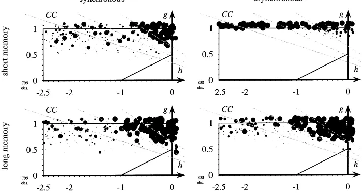
Huberman and Glance (1993) criticise May and Nowak’s model arguing that due to the synchronous dynamics the network might run into cycles that are unstable against small perturbations. They suggest random sequential learning to model more realistic timing. While in each period all possible interactions take place, only one single player learns in a given period. The order in which players learn is determined randomly. In a particular setting,13 where May and Nowak found cooperation, random sequential learning leads to general non-cooperation. They claim that synchronisation is an artificial assumption and can hardly be justified. In Fig. 4 we find that they are right. It is indeed sufficient to go only a small step14 into the direction of the model proposed by Huberman and Glance to notice that cooperation dies out almost completely with short memory and asynchronous interaction.
However, the assumption of short memory made by Huberman and Glance is crucial. Once long memory is introduced (see bottom part of Fig. 4) we find that in both cases, with synchronous or with asynchronous interaction, a range of games where cooperation survives.
We have the following intuition for this phenomenon: A cooperative player can only learn to become a D when there is at least one D in the neighbourhood. In such a period,
13The initial configuration, game, learning rule, etc. correspond to Fig. 3a–c of May and Nowak (1992). 14Huberman and Glance give each period at most one player an opportunity to change the strategy and players
Fig. 4. Non-discriminative strategies with ‘copy best player’. ‘Copy best player’ learning rule, network=80×80,
r=1. Asynchronous learning eliminates cooperation only with ‘short memory’. To save space we display only the relative frequency of mutual cooperation for a variety of models. The top left diagram displays the relative frequency of cooperation in May and Nowak’s model. We have shown this diagram already in Fig. 3. The top right diagram shows the same model, but now with asynchronous learning and interaction as an approximation to Huberman and Glance. Cooperation dies out. The two diagrams at the bottom show the case of long memory where cooperation survives.
however, Cs are particularly unsuccessful. A C with long memory may keep in mind that sometimes there were more Cs being more fortunate and finds C still more attractive than D. A C with short memory only looks at current payoffs, which are bad for C at the moment and, hence, is more likely to become a D. Hence, with short memory, cooperation is more vulnerable.
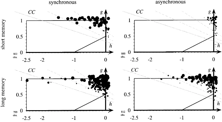
The above simulations were done with the learning rule ‘copy best player’ since this was also the learning rule used by Nowak and May. This particular choice is not es-sential. In Fig. 5 we show the results for the ‘copy best strategy’ learning rule. It turns out that changing the learning rule has little impact on the relative frequency of mutual cooperation.
5.3. The case of discriminative strategies
The non-discriminative strategies discussed above forced players to treat their neighbours without distinction. Either they had to play C or they had to play D against all of them. We will now introduce discriminative behaviour. Players’ strategies will be described as small (two-state) automata. Each player uses only one automaton, but this automaton can be in different states against different neighbours. Results change substantially now.
Fig. 5. Non-discriminative strategies with ‘copy best strategy’. ‘Copy best strategy’ learning rule, network=80×80,
r=1. The only difference to Fig. 4 is that here players use ‘copy best strategy’ as a learning rule. Again cooperation is eliminated only with ‘short memory’.
interesting property of spatial evolution, mutual exploitation. In Section 5.3.2 we proceed to a model where players interact stochastically and learn from long memory.15 The dynamics in the latter model may be harder to analyse, but is also more robust and sometimes more convincing.
5.3.1. Synchronous interaction and short memory
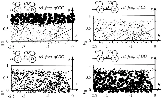
In the following section we assume that learning is asynchronous but that interaction is still synchronised. Players learn from short memory. Let us first look at Fig. 6 which shows simulation results for a population that uses discriminative strategies. Players use the learning rule ‘copy best strategy’ as defined in Section 3.4. We find a larger range of games where cooperation survives with discriminative strategies (in Fig. 6) than with non-discriminative strategies (see Fig. 5). Discriminative strategies, for instance members of a cluster of tit-for-tats, are able to cooperate with their kin in their neighbourhood, but will not be put-upon by Ds. Notice that the range of games where CC prevails is mainly determined by the value ofg, i.e. by the payoff for CC. The value ofh for CD does not have much influence. Reproduction mainly occurs upon successful CCs when past CDs are already forgotten. This will change when we introduce long memory in Section 5.3.2.
In Section 4 we introduced a simple analytical model that could explain how a dis-crete world supports mutual exploitation. In the following paragraph we will corroborate
Fig. 6. Discriminative strategies,pI =1,tL ∈ {10, . . . ,14}, copy-best-strategy, short memory,rL =rI =1,
network=80×80.
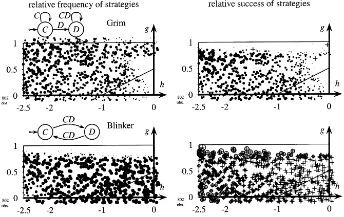
this finding with simulation results. We will consider a population that initially contains all 26 discriminative strategies in random proportions. Two of them, grim andblinker, despite their different average payoff, appear together for a wide range of games. The left-hand part of Fig. 7 shows that both grim andblinker survive for a wide range of payoffs. In the right-hand part we see that grim’s payoff is higher than average for most games while blinker’s payoff is smaller than the average population payoff. We did not observe this phenomenon with non-discriminative strategies, the reason being that in some games all agents played C, in the others they all played D. Hence, they all had the same payoff.
Notice that the above described heterogeneity of payoffs differs from the heterogeneity of strategies pointed out by Lindgreen and Nordahl (1994). They find that spatial evolu-tion yields in contrast to global evoluevolu-tion starting from a homogeneous initial state in the long run a heterogeneous state in the sense that several different strategies are distributed in ‘frozen patchy states’ over the network. In the current and in the following sections we show two related things: First, even a population which has not reached a static state (and will possibly never reach one) can exhibit stable properties, e.g. relative frequen-cies of different strategies that may achieve a stable level. Second, in addition to strate-gies that are distributed heterogeneously over the network, also payoffs of stratestrate-gies are heterogeneous.
Fig. 7. Frequency and success of grim and blinker with synchronous interaction and short memory. Discriminative strategies,pI = 1,tL ∈ {10, . . . ,14}, copy-best-strategy, short memory,rL = rI = 1, network=80×80.
Frequencies are shown in the left-hand side part of the figure as explained in Section 5.1. Relative success is shown in the right-hand side of the figure in the following way: Average payoffs of strategies are calculated over the last 50 periods of a simulation. Black circles indicate that a strategy’s average payoff is larger than population payoff. Crossed white circles indicate that the strategy’s average payoff is smaller than average population payoff. Sizes of the circles are proportional to the payoff difference. When all automata use the same stage game strategy average payoffs per interaction for all automata are identical and no circles and crosses are shown.
the above case and which is discussed in Kirchkamp (1995)) and turn immediately to asynchronous interaction with long memory in the next section.
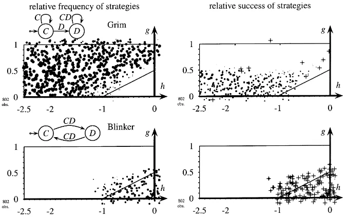
5.3.2. Asynchronous interaction and long memory
Fig. 8. Frequency of CC, CD, and DD encountered by grim. Discriminative strategies,pI=1,tL∈ {10, . . . ,14},
copy-best-strategy, short memory,rL=rI=1, network=80×80, sizes of the circles are proportional to relative
frequencies of strategies. Grim strategies alternate between a small amount of support for their environment, playing CD, and substantial exploitation with DC.
Fig. 10. Frequency and success of grim and blinker with asynchronous interaction and long memory. Discriminative strategies,pI = 12,tL ∈ {20, . . . ,28}, copy-best-strategy, short memory,rL = rI = 1, network=80×80.
Frequencies are shown in the left-hand side part of the figure as explained in Section 5.1. Relative success is shown in the right-hand side part. Average payoffs of strategies are calculated over the last 50 periods of a simulation. Black circles indicate that a strategy’s average payoff is larger than population payoff. Crossed white circles indicate that the strategy’s average payoff is smaller than average population payoff. Sizes of the circles are proportional to the payoff difference. When all automata use the same stage game strategy average payoffs per interaction for all automata are identical and no circles and crosses are shown.
the experience of CDs remains in memory until reproduction occurs, and hence counts for the choice of strategies.
5.4. Coordination games
The same analysis can be applied not only to prisoners’ dilemmas, but also to coordination games. The parameterisation for symmetric coordination games that we have chosen is shown in Fig. 11. The game has two pure equilibria, one where both players play C, and another where both players play D. Both players would prefer to coordinate on one of the two. Harsanyi and Selten (1988) propose two criteria to select among these equilibria. Risk dominance and Pareto dominance. Unfortunately these two criteria do not always pick the same equilibrium.
Fig. 11. Parameterisation for coordination games. The game is a coordination game forg >−1 andh <0. In this case the Pareto dominant equilibrium is CC ifg >0 and DD otherwise. The risk dominant equilibrium is CC if
g >−1−h(denoted CC>riskDD in the figure) and DD otherwise (denoted DD>riskCC in the figure).
In Section 2 we have already studied a simplified model of a continuum of players and considered the situation of a learning player whose left neighbours all play C and whose right neighbours all play D. A myopically optimising player calculates that chances to meet either a C or a D are equally12and therefore selects the risk dominant equilibrium. A player who, however, imitates successful strategies will in the same situation become a C if
g > (1+h)n−4
4+n (7)
wheren ≤ 2 describes the size of the cluster. Clusters with a diameter larger than two times the neighbourhood radius can be treated asn=2. Since coordination games favour large clusters we concentrate on the casen = 2.16 The grey line in Fig. 12 describes the set of games where g = −13(1+h), i.e. the case where for n = 2 we have g = (1+h)(n−4)/(4+n). It is almost precisely the lineg= −13(1+h)which divides the region where only C is played from the region where only D is played. CDs which fail to coordinate are extremely rare. The continuous model described in Section 2 explains the behaviour of the discrete population substantially better than Pareto dominance or risk dominance.
5.5. The influence of locality
So far we assumed that learning and interaction were within a neighbourhood of radius 1. Fig. 13 shows the amount of mutual cooperation for larger neighbourhoods. Starting from rI=rL=1, we enlarge neighbourhoods for learning and interaction simultaneously until we reach global interaction and learning. With less locality the range of games where CC is played becomes gradually smaller. We have done further simulations where we keep the
16In a prisoners’ dilemma clusters are often small since only small groups of defectors are successful. As soon
Fig. 13. Frequency of CC depending on the size of the neighbourhood.r=rI =rL, discriminative strategies,
pI=12,tL∈ {20,28}, copy-best-strategy, long memory, network=21×21. The population is smaller (21×21)
Fig. 14. Frequency of CC in one- to four-dimensional networks. Discriminative strategies, pI = 12,
tL ∈ {20, . . . ,28}, copy-best-strategy, long memory. Notice that neighbourhoods are about 10 times as large
than in the above simulations. This explains that the cooperative area is smaller than in Fig. 9.
learning radiusrLconstant and vary the interaction radiusrIor vice versa and found that both locality of evolution and locality of interaction smoothly increase the range of games where cooperation prevails.
5.6. Other dimensions
Beyond the results that we presented above we have carried out many further simulations, each showing that the effects that we pointed out here persist for several modifications of the model. One possible modification is the change from a two-dimensional torus to tori with other dimensions. Fig. 14 shows the relative frequency of mutual cooperation in one- to four-dimensional networks. All networks have 4096 players and all neighbourhoods have almost the same number (80, . . . ,125) of opponents. We see that the dimension of the network has almost no effect on the size of the cooperative area.
6. Concluding remarks
We have analysed a simple model of spatial evolution where agents repeatedly play prisoners’ dilemmas and coordination games.
of using more complex strategies might move quicker to a more rational solution. We find, however, that more complexity fosters cooperation.
We further observe inequality of payoffs among coexisting strategies. While global evolu-tion predicts that strategies with lower than average payoff die out, local evoluevolu-tion explains symbiosis of strategies where one strategy alternates between slightly feeding and substan-tially exploiting the other.
We respond to a criticism raised by Huberman and Glance (1993) who argue that asyn-chronous timing might eliminate cooperation completely. We find that their argument cru-cially depends on their assumptions about memory of players. As soon as players have long memory cooperation survives both with asynchronous as well as with synchronous timing. We further extend the analysis of Huberman and Glance (1993) and Bonhoeffer et al. (1993) allowing not only for asynchronous learning but also for asynchronous interaction. We find that this avoids that the evolutionary process gets stuck in odd patterns of behaviour. We find that some properties of a discrete local model can be approximated by a continu-ous one that is easier to analyse. The approximation of the continucontinu-ous model is surprisingly accurate in particular for coordination games.
Acknowledgements
Support by the Deutsche Forschungsgemeinschaft through SFB 303 and SFB 504 is gratefully acknowledged. I thank George Mailath, Georg Nöldeke, Karl Schlag, Avner Shaked, Bryan Routledge, several seminar participants and two anonymous referees for helpful comments.
Appendix A. Proof of Proposition 1
In the following we will denote a pair of two automataaandbwith the symbolha, bi. For notational convenience we will make no distinction betweenha, biandhb, ai
1. If there are only grims in the population, then onlyhGC, GCi,hGC, GDiandhGD, GDi
are possible.hGC, GDiis unstable, thus, onlyhGC, GCiandhGD, GDiwill remain in the population. Given any relative frequency ofhGC, GCiandhGD, GDino player will ever learn, since there are no alternative strategies to observe.
2. If there are only blinkers in the population, then only⌈hBC, BCihBD, BDi⌉,⌈hBD, BDi
hBC, BCi⌉and⌈hBC, BDi⌉are possible. All of these cycles of pairs are stable. No player will ever learn, since there are no alternative strategies to observe.
3. Trivially a state where possibly payoffs cycle, but nevertheless in all periods grim and blinker achieve the same payoff is an equilibrium, since no player ever has any rea-son to learn. An example for such an equilibrium is a population where 14 are cycles
⌈hBC, BCihBD, BDi⌉, 14 are cycles⌈hBD, BDihBC, BCi⌉,(1+h)/4gare⌈hGC, GCi⌉
Fig. 15. Transitions of cycles of stable pairs if payoffs cycle like⌈ ¯uB>u¯G,u¯G>u¯B⌉. Transitions with speed 2ǫ are shown with double lines. Speedǫis shown with single lines. Transitions that take place in the second period are shown with dashed (single or double) lines. The first period is shown with solid lines.
This equilibrium is not stable. Change the relative frequency of a cycle that contains blinkers only slightly and payoffs of blinkers start cycling around the average population payoff. In the discussion of case 4 which is described below we will see that once such a state is reached, the cycling becomes stronger and stronger until the equilibrium of case 4 is reached.
4. hGC, GCi,hGD, GDi,hGD, BDi,hBD, BDi,hBC, BCiall belong to a stable cycle in the sense that after a limited number of transitions each pair will return to its original state. Unstable pairs are the remaining oneshGC, GDi,hGC, BCiandhGC, BDi. Unstable pairs can only be present in a cyclical equilibrium if they are introduced through learning. Since we take the limit of the learning rateǫ → 0, the relative frequency of unstable pairs in the population will be zero as well. Thus, in a cyclical equilibrium we have only stable pairs.
All stable pairs belong to cycles of length either one or two. Therefore average payoffs in a cyclical equilibrium also form a cycle of length either one or two.
A cyclical equilibrium with both grim and blinker present in the population must have average payoffs of grim and blinker belonging to a cycle of length two. Otherwise one strategy would have always more than average payoff, which together with our learning rule, copy always the best average strategy, leads to the extinction of the other strategy. Let us without loss of generality assume that average payoffs form a cycle of length two with ⌈ ¯uB > u¯G,u¯G > u¯B⌉. Thus, in the first period of each cycleu¯B > u¯G,
in the secondu¯G > u¯B. Fig. 15 shows now the dynamics of stable pairs. Let us give
one example how to determine the transitions. There is some flow away from the cycle
When we consider all transitions given in Fig. 15 we see that only the three cycles Now let us look at the payoffs. In the first period of a cycle almost all pairs play DD, i.e. they get, given the game in Fig. 1, a payoff of zero. Nevertheless, a few pairs are always present which actually learned a new strategy. Thus, we have 12ǫofhGC, GDi and12ǫofhGC, BDi. Therefore payoffs are in the first period of a cycle as follows:
¯
uG= 12ǫ(1+2h) < u¯B= 12ǫ
In the second period of a cycle learning players are negligible:
¯
uG= 12 > u¯B= 12(g+h)
Thus, indeed a cycle of payoffs like⌈ ¯uB>u¯G,u¯G>u¯B⌉exists.
References
Ashlock, D., Stanley, E.A., Tesfatsion, L., 1994. Iterated prisoner’s dilemma with choice and refusal of partners. In: Langton, C.G. (Ed.), Artificial Life III, No. XVII in SFI Studies in the Sciences of Complexity. Addison-Wesley, Reading, MA, pp. 131–167.
Axelrod, R., 1984. The Evolution of Cooperation. Basic Books, New York.
Bonhoeffer, S., May, R.M., Nowak, M.A., 1993. More spatial games. International Journal of Bifurcation and Chaos 4, 33–56.
Ellison, G., 1993. Learning, local interaction, and coordination. Econometrica 61, 1047–1071.
Eshel, I., Samuelson, L., Shaked, A., 1998. Altruists, egoists, and hooligans in a local interaction model. The American Economic Review 88, 157–179.
Harsanyi, J.C., Selten, R. 1988. A General Theory of Equilibrium Selection in Games. MIT Press, Cambridge, MA.
Hegselmann, R., 1994. Zur Selbstorganisation von Solidarnetzwerken unter Ungleichen. In: Homann, K. (Ed.), Wirtschaftsethische Perspektiven I, No. 228/I in Schriften des Vereins für Socialpolitik Gesellschaft für Wirtschafts und Sozialwissenschaften Neue Folge. Duncker and Humblot, Berlin, pp. 105–129.
Hotelling, H., 1929. Stability in competition. Economic Journal 39, 41–57 .
Huberman, B.A., Glance, N.S., 1993. Evolutionary games and computer simulations. Proceedings of the National Academy of Sciences 90, 7716–7718.
Kandori, M., Mailath, G.G., Rob, R., 1993. Learning, mutation, and long run equilibria in games. Econometrica 61, 29–56.
Kirchkamp, O., 1995. Spatial evolution of automata in the prisoners’ dilemma. Discussion Paper B-330, SFB 303. Rheinische Friedrich Wilhelms Universität Bonn.
Lindgreen, K., Nordahl, M.G., 1994. Evolutionary dynamics of spatial games. Physica D 75, 292–309. May, R.M., Nowak, M.A., 1992. Evolutionary games and spatial chaos. Nature 359, 826–829.
May, R.M., Nowak, M.A., 1993. The spatial dilemmas of evolution. International Journal of Bifurcation and Chaos 3, 35–78.
Maynard Smith, J., Price, G.R., 1973. The logic of animal conflict. Nature 273, 15–18.
Sakoda, J.M., 1971. The checkerboard model of social interaction. Journal of Mathematical Sociology 1, 119–132. Schelling, T., 1971. Dynamic models of segregation. Journal of Mathematical Sociology 1, 143–186.
Taylor, P.D., Jonker, L.B., 1978. Evolutionary stable strategies and game dynamics. Mathematical Biosciences 40, 145–156.
Young, H.P., 1993. The evolution of conventions. Econometrica 61, 57–84.