Visualizing Water Quality Sampling-Events in Florida
M. D. Bolt*, Oak Ridge Institute of Science and Education /U.S. Environmental Protection Agency Sam Nunn Atlanta Federal Center 61 Forsyth Street, SW Atlanta, GA 30303 United States - [email protected]
KEY WORDS: Water Quality, Visualization, Florida, R, GIS, Spatiotemporal, Communication
ABSTRACT:
Water quality sampling in Florida is acknowledged to be spatially and temporally variable. The rotational monitoring program that was created to capture data within the state’s thousands of miles of coastline and streams, and millions of acres of lakes, reservoirs, and ponds may be partly responsible for inducing the variability as an artifact. Florida’s new dissolved-oxygen-standard methodology will require more data to calculate a percent saturation. This additional data requirement’s impact can be seen when the new methodology is applied retrospectively to the historical collection. To understand how, where, and when the methodological change could alter the environmental quality narrative of state waters requires addressing induced bias from prior sampling events and behaviors. Here stream and coastal water quality data is explored through several modalities to maximize understanding and communication of the spatiotemporal relationships. Previous methodology and expected-retrospective calculations outside the regulatory framework are found to be significantly different, but dependent on the spatiotemporal perspective. Data visualization is leveraged to demonstrate these differences, their potential impacts on environmental narratives, and to direct further review and analysis.
1. INTRODUCTION
Florida contains thousands of miles of freshwater streams and coast, and millions of acres of lakes, ponds, and reservoirs for which the state is responsible. This represents approximately 13.6 ft. of streams and 4,575 sq. ft. of lakes per Floridian (USEPA, 2000 and U.S. Census, 2015). Additionally, sharing these resources are 269 endemic species of 4,368 known species in the Sunshine State (Bruce, 2002). This biological bounty ranks Florida 4th in the nation for endemism and 7th for biodiversity. Despite their growing wealth of environmental data, not every water body can be sampled every year within this water rich and biodiverse state.
1.1 Sampling in Florida
Due to practical time and manpower constraints sampling in Florida is completed on a 5 group and cycle rotation program. Groups are constituted from a collection of basins from across the state, such that no quadrant of the state receives more assessment focus in a cycle than another. Cycles contain two significant regulatory components: a planning period of 10 years and a verified period of 7.5 years. Basins have stable boundaries and are internally comprised of regulatory assessment units: the Water Body IDentification unit (WBID). Containing none or more stations, WBIDs subdivide basins as contiguous spatial extents. Station data within WBIDs are aggregated to the assessment unit for application in regulatory assessment. In streams and coastal areas dissolved oxygen (DO) is reported as a calculated daily average. Stations do not move in space, but their use may vary throughout time – with locations commissioned or decommissioned for a bevy of reasons. WBIDs, however, may move within the boundaries of the basins. WBID boundaries and water body type too can be refined by the Florida Department of Environmental Protection (FDEP) to more accurately define water bodies for regulatory assessment purposes. In this way stations may change WBID designation without moving. Within the WBID refinement and group-cycle processes, sampling must also be applied by FDEP to maximize both human and environmental protection. Approaching the resulting system through the lens of a
water quality standard methodology change, Dissolved Oxygen (DO) to Dissolved Oxygen Saturation Percent (DOSat%), allows for a brief view of the impact sampling efforts can have on environmental quality narratives.
1.2 A New Standard
As part of ongoing and dedicated work by the local, state, and federal agencies, advocacy groups, and citizen scientists that shape the policy applied in Florida, a new DO assessment methodology and standard was developed for the state: DOSat%. This new standard recognizes ecosystem factors that can contribute to changes in the potential maximum DO within a given sample. These were determined, by FDEP, to primarily include temperature, barometric pressure, and conductivity or salinity. As these factors vary in response to change in the environment, so too does DO. How this standard is applied to assess for water quality impairment varies between water body types- in both collection frequency and perspective. For example, DOSat% in marine waters is viewed from daily, weekly, and monthly perspectives whereas streams are viewed at the daily step (FDEP, 2015). This study focuses on the daily perspective that is common to both the streams and coastal sampling.
not have changed. This study focuses on this aspect of the process, potential pitfalls, and how to best generally communicate the influence of sampling–event behaviors to a varied audience.
In the U.S., questions about environmental quality are approached from multiple levels and backgrounds via regulators, scientists, citizen activists, industry, etc. Included in the pursuit of best available approaches is the inherent problem of addressing access and consensus building within a broad audience and the additional issue of avoiding perception and environmental memory ratchets (Pitcher, 2001 and Kahn, 2002). As suggested by Host (2000), how much can visualization assist broader audiences to access information while addressing shifting perceptions in the face of shifting standards? This study leverages the opportunity created in the Florida water quality standard shift to address these questions and assertions.
2. DATA & METHODS
Data was delivered via MS-Access, manipulated and analyzed in MS-Excel, and visualized in R and ESRI ArcGIS. The GoogleVis package from the CRAN library was used to visualize data with R.
2.1 Data
The primary coastal and stream environmental quality data was retrieved from the Florida Integrated Water Quality Assessment Report, which is a product of that state’s Impaired Waters Rule (IWR). Each cycle and any additional site specific sampling events within that cycle are included in an updated “Run”. Each Run is a snapshot of the WBIDs, new data, and all data preceding which is packaged into an MS-Access database. The file is publicly
available from the FDEP website and reflects their total sampling efforts to date.
The most recent IWR Run, number 49, was chosen. Due to the dynamic nature of WBIDs, their discussion and inclusion here is for reference only. The WBID delineation is set by Run 49 and does not reflect past permutations; station and basin data received primary focus. This places the study findings outside meaningful regulatory spatial framework. Annual reporting was complete up to and including 2012, thus the data in this study ranges from 1905-2012. Additional and incomplete data for 2013 and 2014 that exist in the IWR was not included. For the purposes of this study, sampling is viewed as a continuous record.
daily, and included. The pDOSAT data was combined with the IWR data and summarized to daily station-sampling-events per basin for DO and pDOSAT. The data was then viewed from varying temporal perspectives.
2.2 Methods
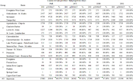
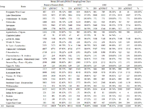
2.2.1Descriptive Analysis Using MS-Excel (2013), a descriptive table comparing daily station sampling events for pDOSAT and DO per basin, per year was created (Tables 1, 2). This study focuses on four time intervals which: the Period of Record (PoR), the early years of Clean Water Act implementation (1975-2012), renewal impacts (1980-2012), and the adoption of the Florida Impaired Waters Rule program (2001-2012).
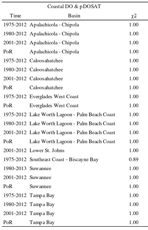
2.2.2Chi Square The basin and group aggregated coastal waters and streams DO and pDOSAT data was analyzed across the time periods of note, via Chi Square test for Independence. (Tables 3, 4) All analysis was conducted in MS-Excel.
2.2.3R Coastal and stream daily sampling data sets, including the above parameters and the calculated pDOSAT, were loaded into R (i386 3.1.2). Data was converted into a dataframe and date fields were converted from MS-Excel format to R format. Using the GoogleVis package (0.5.6), coastal and stream data for the entire record were visualized into two motion charts: stream and coastal.
2.2.4 GIS The data loaded into R in 2.2.3 was also imported into ESRI ArcGIS using the Excel to Table tool. The table’s coordinate data was displayed and projected onto a WBID layer from FDEP. The result was converted to a shapefile, and “Time” was enabled which allows for use of the Time Slider.
3. RESULTS
3.1 Descriptive Analysis
The descriptive analysis revealed a greater agreement between DO and pDOSAT stream sampling events in more recent years. Within the entire period of record, there is a considerable 25% spread which tightens to a 3% spread in the 2001-2012 or IWR adoption period. (Table 2). Coastal data, with the exception of the recent sampling events in the Choctawachee-St. Andrew basin, follow the same pattern as stream data in closing the spread between DO and pDOSAT sampling events. Here the spread moves from 11% to 1% across temporal scales (Table 1).
3.2 Chi Square
Analysis of the period of record for both streams and coastal waters reveals significant difference between DO sampling and pDOSAT. The significance of the component groups and temporal scales, however, is more complex (Table 3, 4). Where possible due to data constraints imposed by analytical methods, further analysis of the constituent basins does not reveal a significant difference between the data sets (Table5, 6).
3.3Motion Charts
When pDOSAT and DO are visualized in the multivariate space of the motion chart discrepancies in spatial and temporal sampling event distribution are identifiable (Figures 1). Localized sampling event phenomenon, such as legacies of specific campaigns, can also be identified.
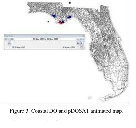
3.4 Animated Maps
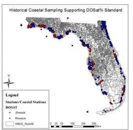
Similar to the motion charts, discrepancies were visible when size and color of sampling-days represented combinations of pDOSAT and DO. This was seen somewhat in the static maps, but was more prominent in the animated map of the coastal sampling. The variability and frequency of coastal and stream sampling was more
apparent within the spatiotemporal space provided by the map (Figure 2, 3).
4. DISCUSSION & CONCLUSION
Loaning from Pitcher’s (2001) description of well-known environment and resource perception ratchets in fisheries and Kahn’s (2002) work on environmental amnesia we can recognize there are potential traps inherent in handling environmental data. These traps can begin to be avoided by understanding the progression of environmental quality at varying scales through time. Similarly, accessing the interconnected behaviors of environmental quality parameters is important to understanding their progression. This is reflected in the mathematical underpinnings of the DOSat% standard which recognizes the influence of temperature, salinity, and conductivity upon the potential for DO within a sample. These parameters are often themselves a proxy for the influence of a host of constituents. Thus, in addition to the complexities within the study system, those Table 4. Stream DO & pDOSAT Chi Square test for
Independence. Test was conducted at various spatial and temporal scales.
Comparisons Period of Record 1975-2012 1980-2012 2001-2012 All Basins 2.8 x 10-38 0.009 0.999 1
Stream DO & pDOSAT Sampling Events
Comparisons Period of Record 1975-2012 1980-2012 2001-2012
All Basins 2.446 x 10-42 4.742 x 10⁻²⁸ 1.348 x 10⁻²⁷ 1.350 x 10⁻²⁷
Coastal DO & pDOSAT Sampling Events
Table 3. Coastal DO & pDOSAT Chi Square test for Independence. Test was conducted at various spatial and
temporal scales.
1975-2012 Lake Worth Lagoon - Palm Beach Coast 1.00
1980-2012 Lake Worth Lagoon - Palm Beach Coast 1.00
2001-2012 Lake Worth Lagoon - Palm Beach Coast 1.00
PoR Lake Worth Lagoon - Palm Beach Coast 1.00
2001-2012 Lower St. Johns 1.00
1975-2012 Southeast Coast - Biscayne Bay 0.89
1980-2013 Suwannee 1.00
Table 5. Coastal DO & pDOSAT basin level analysis. Chi square test for independence was applied to those basins that
imposed by sampling can have an additional influence. In both short term sampling cycles and over the entire period of record there appears to be a sampling influence asserted.
4.1 Statistical Analysis
As is seen in the descriptive statistics, in keeping with Odum’s ratchet, sampling behavior at the state and basin level may not always align (Pitcher, 2001). For example, over the period of record, 96% and 97% of all DO and pDOSAT sample events agree in streams and coastal bodies respectively; however there is great variability of sample event agreement at the basin level within the same period. This is also played out in the Chi square analysis at the state, intergroup, intragroup, and basin scales (Tables 3, 4, 5, 6). These results highlight the impact of upscaling and aggregating practices, across space and time. Further analysis of the specific drivers behind this pattern is needed, specifically reviewing for spatiotemporal sensitivity.
It is important to note that this study focuses on two of the four types of water bodies identified in the IWR Run 49. The variations in basin spatial extent, in addition to basin makeup, may account for the order of magnitude variation between sampling. Viewing the sampling behavior of all water bodies within a basin would aid in further overcoming perception traps. This is also true when reviewing sampling results, due to the connectivity between these systems. This study’s analysis recognizes and applies the regulatory use of daily averages. How this process may affect the ability to identify significant but temporal phenomena and whether data currently exist to support such analysis requires additional work at more fine spatial and temporal scales.
4.2 Visualization
As noted in Host et al (2000) and Silberbauer (2009) there is both a need for quick and broadly accessible data communication of complex issues surrounding environmental quality information. Both of those studies and this one recognize the limitations in visual inspection to determine significance. Similarly, there exists a possibility of drawing spurious conclusions from visual inspection that should be confirmed statistically. Countering these concerns, is the ability of visualization to assimilate large amounts of data over long periods in an accessible manner.
As in Figures 1-3 Florida’s entire record of daily coastal DOSat% constituent parameters, and pDOSAT were visualized in two different programs. Stream data was also visualized in this manner; stream visualization images were not included for the sake of
Time Basin χ2
1975-2012 Caloosahatchee 1.0000
1980-2012 Caloosahatchee 1.0000
PoR Caloosahatchee 1.0000
1975-2012 Charlotte Harbor 0.9801
1980-2012 Charlotte Harbor 0.9811
1975-2012 Fisheating Creek 1.0000
1980-2012 Fisheating Creek 0.9990
2001-2012 Fisheating Creek 0.9990
PoR Fisheating Creek 1.0000
1975-2012 Kissimmee River 1.0000
1980-2012 Kissimmee River 1.0000
2001-2012 St. Lucie - Loxahatchee 1.0000
1975-2012 Tampa Bay 0.8574
PoR Withlacoochee 1.0000
Stream DO & pDOSAT
Table 6. Stream DO & pDOSAT basin level analysis. Chi square test for independence was applied to those basins that could support the test to
illustrate scalar differences.
Figure 1 . Coastal DO and pDOSAT motion chart.
brevity. Figure 1 demonstrates the behaviors identified in the five variable space that motion charts provide. Depicted is December 15, 2007 with large red circles signaling recent DO findings that coincide with pDOSAT. The smaller blue dots identify a recent sampling that does not include DO and does not meet the requirements for pDOSAT. A drawback to this visualization process is the “hang time” of the circles which the program interprets as integer data for smoothing purposes. In both stream and coastal motion charts changes in sampling frequency, latitude, longitude, spatial extent, and constituency are apparent through time. Areas with less data are easily recognizable in some combinations- as in the above which shows a momentary gap in the Suwanee basin. The change in the relationship between DO and pDOSAT is noticeable when viewed in this manner. Other phenomenon are apparent, such as abrupt lack of sampling during major weather events.
GIS data visualization shown in Figure 2 displays the entire record of Florida’s coastal sampling, statically stacked. Here larger red circles also identify points where pDOSAT was supported and DO reported. Likewise, smaller blue circles are points where neither DO was reported nor pDOSAT supported. This creates a 4 variable representation (latitude, longitude, pDOSAT, DO) or 5 if including spatial relationships. Figure 3 animates that map, providing the additional variable of time. The data seen in place over their respective WBIDs adds an additional variable. With this visualization tool some patterns are identifiable and noticeable prior to statistical review. This arrangement of geospatial data is also ripe for conversion for spatial statistical analysis which may yield further insight into sampling behavior and the possibility for sample bias.
As tools for communicating data behavior, both motion charts and animated maps provided unexpectedly supportive views of statistically identified trends. The inclusion of the entire record of Florida’s sampling for pDOSAT constituents and DO creates a compelling look at the progression of stream and coastal water quality sample-events throughout the last approximately 90 years. Further research and work on combining these data visualizations into a robust suite of communication and consensus building tools should be conducted in addition to the work already completed (Host, 2000; Boyer, 2000; and Halls 2003). Regulatory
perspectives on applicability to ongoing discussions should be explored.
ACKNOWLEDGEMENTS
This project was supported in part by an appointment to the Research Participation Program at the Office of Water, U.S. Environmental Protection Agency, administered by the Oak Ridge Institute for Science and Education through an interagency agreement between the U.S. Department of Energy and EPA
REFERENCES
Boyer et al. 2000. Maximizing Information from a Water Quality Monitoring Network through Visualization Techniques.
Estuarine, Coastal and Shelf Science, 50, pp. 39–48.
Bruce, A.S. 2002. States of the Union: Ranking America’s Biodiversity. NatureServe, Arlington, Virginia, USA.
FDEP (Florida Department of Environmental Protection). 2008. Florida Administrative Code. Chapter 62.303.
https://www.flrules.org/gateway/ChapterHome.asp?Chapter=62-303 (1 Jan. 2015).
Halls, J. N. 2003. River run: an interactive GIS and dynamic graphing website for decision support and exploratory data analysis of water quality parameters of the lower Cape Fear river. Environmental Modeling & Software, 18, pp. 513-520.
Host. 2000. Interactive Technologies for Collecting and Visualizing Water Quality Data. URISA Journal, 12, (3), pp. 39.
Kahn, P. J. 2002. Children and Nature: Psychological, Sociocultural, and Evolutionary Investigations. MIT Press, Cambridge MA. Chp 4
Pitcher, T. J. 2001. Fisheries managed to rebuild ecosystems? Reconstructing the past to salvage the future. Ecological Applications, 11(2), pp. 601-617.
Silberbauer, MJ. 2009. Using the Google Gapminder motion chart gadget to visualise long-term chloride-to-sulphate ratios in South African rivers. South African Society of Aquatic Scientists: Beyond rapid assessments – time for an aquatic research renaissance in South Africa. Poster. Broederstroom, South Africa. https://www.dwaf.gov.za/iwqs/water_quality/NCMP/method/Goo gle_Gadget_Water_Quality_region_colour.pdf (3 Apr 2015)
USEPA (U.S. Environmental Protection Agency). 2000. 2000 National Water Quality Inventory. EPA-841-R-02-001 WASHINGTON, DC.
U.S. Census Bureau. 2015. U.S. Census Bureau: State and County QuickFacts. Data derived from Population Estimates, American Community Survey, Census of Population and Housing, State and County Housing Unit Estimates, County Business Patterns, Nonemployer Statistics, Economic Census, Survey of Business Owners, Building Permits.