ENHANCEMENT OF GENERIC BUILDING MODELS BY RECOGNITION AND
ENFORCEMENT OF GEOMETRIC CONSTRAINTS
J. Meidow∗, H. Hammer, M. Pohl, D. Bulatov
Fraunhofer IOSB, Ettlingen, Germany - (jochen.meidow, horst.hammer, melanie.pohl, dimitri.bulatov)@iosb.fraunhofer.de
Commission III, WG III/4
KEY WORDS:Building Model, Reasoning, Adjustment, Boundary Representation, 3D City Models
ABSTRACT:
Many buildings in 3D city models can be represented by generic models, e.g. boundary representations or polyhedrons, without ex-pressing building-specific knowledge explicitly. Without additional constraints, the bounding faces of these building reconstructions do not feature expected structures such as orthogonality or parallelism. The recognition and enforcement of man-made structures within model instances is one way to enhance 3D city models. Since the reconstructions are derived from uncertain and imprecise data, crisp relations such as orthogonality or parallelism are rarely satisfied exactly. Furthermore, the uncertainty of geometric entities is usually not specified in 3D city models. Therefore, we propose a point sampling which simulates the initial point cloud acquisition by air-borne laser scanning and provides estimates for the uncertainties. We present a complete workflow for recognition and enforcement of man-made structures in a given boundary representation. The recognition is performed by hypothesis testing and the enforcement of the detected constraints by a global adjustment of all bounding faces. Since the adjustment changes not only the geometry but also the topology of faces, we obtain improved building models which feature regular structures and a potentially reduced complexity. The feasibility and the usability of the approach are demonstrated with a real data set.
1. INTRODUCTION
1.1 Motivation
Scenes of arbitrary complexity can be described by generic mod-els, e.g. boundary representations or polyhedrons respectively, in context of modeling man-made objects. Unfortunately, represen-tations obtained by purely data-driven approaches cannot distin-guish between buildings and non-building objects since they con-tain no building-specific knowledge. Actually, data-driven ap-proaches are unable to recognize man-made objects at all but fea-ture the flexibility to capfea-ture objects of arbitrary shape. Specific models, e.g. parametric models, can be directly related to build-ings. Still, being too specific has the disadvantage of restricting the number of representable buildings. In general we have the classical dilemma of choosing a generic, but too unspecific, or a specific, but too restrictive model (Heuel and Kolbe, 2001).
Several concepts exist to introduce building shape knowledge without being too restrictive. In (Xiong et al., 2015) for in-stance, the topological graphs of roof areas are analyzed to com-bine and instantiate predefined building primitives. Another way is to recognize man-made structures by a hypothesis generation-and-testing strategy. Geometric and topological relations such as orthogonality or parallelism are found by statistical hypothesis testing and then established by an adjustment (Meidow, 2014).
To perform the adjustment, a set of consistent and non-redundant constraints is required. Here, consistency refers to non-contra-dicting constraints and redundancy to independent constraints. Thus selection strategies are required to obtain such minimal sets reliably. Conceivable approaches are automatic theorem proving (Loch-Dehbi and Pl¨umer, 2009, Meidow and Hammer, 2016) or decisions drawn on numerical criteria within a greedy algorithm (Pohl et al., 2013).
∗Corresponding author
205 210
215 220
225 230
450 460
470 480 235
240 245 250
✍✌ ✎☞
❳ ❳❳
❳ ❳
❳❳ ❳
❳ ❳❳③
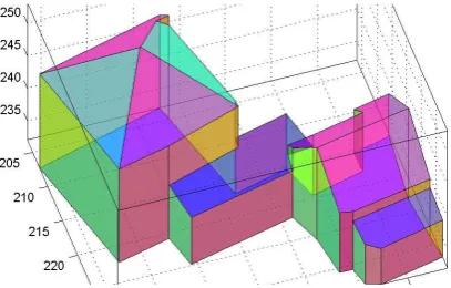
Figure 1: The pyramidal broach roof has been reconstructed as a hipped roof with a very short ridge line. The adjustment pro-cess enforces the concurrence constraint and therefore changes the topology of the roof to a pyramidal roof.
1.2 Contribution
Given the generic model of a building in a boundary representa-tion, we recognize geometric relations such as orthogonality or parallelism automatically by hypothesis testing and enforce the recognized constraints by an efficient adjustment procedure. As a result, we obtain enhanced building models with regular struc-tures and potentially simplified topology.
An example is shown in Figure 1: A pyramidal broach roof is ini-tially represented by a hipped roof at which the ridge line is very short. After recognizing that four planes share a common point with high probability, an adjustment enforcing this constraint has been carried out. This leads to a pyramid as a more appropriate roof description.
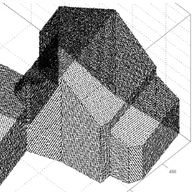
Figure 2: Detail of a point cloud obtained by airborne laser scan-ning and the derived generic polyhedral building reconstruction.
point cloud which simulates the result of an airborne laser scan-ning. Estimates for the plane parameters are obtained from these point clouds which are then the basis for the subsequent reason-ing process.
For the recognition of constraints only the data-independent sig-nificance level, i.e. the probability of correctly not rejecting a null hypothesis, has to be specified. The usability and the feasibility of the approach are demonstrated by the analysis of a generic boundary representation for a building captured by airborne laser scanning. The reconstruction has been carried out according to the approach proposed in (Xiong et al., 2014), cf. Figure 2.
1.3 Related Work
We consider the approach proposed in (Xiong et al., 2014) as one of the most recent methods to derive polyhedral building models from airborne captured point clouds. Formulations for constraints as multivariate polynomials can be found in (Bren-ner, 2005). Constraints and statistical tests for geometric enti-ties in homogeneous representation are provided by (Heuel, 2004, F¨orstner et al., 2000). In (Pohl et al., 2013), a greedy algorithm is used to select a set of independent and consistent constraints au-tomatically. An adjustment model to solve constrained problems formulated in homogeneous coordinates efficiently can be found in (Meidow, 2014). In (Dehbi and Pl¨umer, 2011, Loch-Dehbi and Pl¨umer, 2009) independent constraints are found by automatic theorem proving using Wu’s method (Wu, 1986). The feasibility is demonstrated but no real data sets have been ana-lyzed.
2. THEORETICAL BACKGROUND
After the explanation of the point sampling process and the deter-mination of adjacent point groups (Subsection 2.1) we explain the utilized parametrization of planes and the corresponding param-eter estimation (Subsection 2.2) and formulate geometric con-straints (Subsection 2.3). The recognition of man-made struc-tures by hypothesis testing (Subsection 2.4) and the enforcement of the recognized constraints by an adjustment (Subsection 2.5) are then the core of the reasoning process. Within this approach, the deduction of a set of consistent and non-redundant constraints is essential (Subsection 2.6).
2.1 Point Sampling and Adjacencies
The uncertainties of the geometric entities are required for the complete reasoning and adjustment process. This refers to the statistical testing of geometric relations (Subsection 2.4) as well as to the adjustment of the planes (Subsection 2.5). Thus the un-certainties of bounding planes have to be specified by covariance
Figure 3: Result of the point sampling for each face of the bound-ary representation (bird’s eye view) with sampling distance 20 cm andσ= 3cm for each coordinate. The points of the bottom area have been omitted for clarity.
matrices. Since we assume that the model does not come along with this information, we perform a point sampling for each face of the boundary representation. This sampling simulates the re-sult of the laser scanning initially used for the acquisition of the given model.
Figure 3 shows an exemplary part of the point sampling. For each face, points on a grid with given spacing have been gener-ated. Then noise has been added to the point coordinates. The simulated point cloud of a model face is used to estimate the val-ues of the plane parameters (Subsection 2.2). Furthermore, the point clouds can easily be used to determine the adjacencies of bounding faces which are then used for hypothesis generation. Note that in this way relations can be established which are not contained in the boundary representation at hand.
2.2 Representation of Planes and Parameter Estimation
A convenient representation of a plane is its normal vectorN
withkNk= 1and the signed distanceDof the plane to the ori-gin of the coordinate system. The corresponding homogeneous 4-vector is
A=
N −D
=
Ah
A0
(1)
with its homogeneous partAhand its Euclidean partA0. Since (1) is an over-parametrization, we need to introduce additional constraints for the plane parameters to obtain unique results within the adjustment. We use the spherical normalized vector
A= A
kAk (2)
with corresponding covariance matrix Σ
AA = JΣAAJT ac-cording to error propagation, the covariance matrixΣAAof the unconstrained plane parameters and the Jacobian
J= A
kAk
I4−
AAT ATA
. (3)
For the adjustment we need the spherical normalization (2) as a constraint for the parameters which reads
1 2
ATA−1= 0 (4)
with the factor 1/2 for convenience.
constraint polynomials m
identity d≡=
Ah×Bh
A0Bh−B0Ah
=0 3
verticality d|= [0,0,1,0]A= 0 1
orthogonality d⊥=AThBh= 0 1
parallelism dk=Ah×Bh=0 2
concurrence d◦= det([A,B,C,D]) = 0 1
Table 1: Potential geometric relations between planesA,B, C andDexpressed by multivariate polynomials and the number of independent equations (degrees of freedomm).
pointXi has covariance matrix σ2iI3 with the3×3 identity matrixI3 and standard deviationσi for the coordinates of the
point. The plane passes through the weighted centroid and its normal is the eigenvector belonging to the smallest eigenvalue of the empirical covariance or moment matrixMof the point group.
The covariance matrix of the plane parameters can be derived from the eigenvalues ofM, too (F¨orstner and Wrobel, 2017). The4×4 covariance matrix is full and singular, nevertheless the information is considered completely by the adjustment model presented in Subsection 2.5.
2.3 Formulation of Constraints
With the homogeneous representation of planes, the formulation of constraints is simple. Table 1 summarizes the considered rela-tions between planes, see (Heuel, 2004) for details. The concur-rence constraint states that a 3D point is incident to four planes.
Further specific constraints such as identical slopes for roof areas or horizontal roof ridges are conceivable. But often these con-straints are implicitly already given, which limits their practical relevance, depending on the specific application.
For the recognition of constraints by hypothesis testing and for the enforcement of constraints by adjustment, we need the Ja-cobians of the constraints listed in Table 1. These are sim-ple and can be provided analytically. For the concurrence con-straint∂det(M)/∂vec(M) = adj(M)holds, whereadj(M) is the adjugate of the matrixM = [A,B,C,D]andvec(M) = [AT,BT,CT,DT]T.
2.4 Recognition of Man-Made Structures
For each bounding face, a point cloud is sampled simulating the scanning results. Two point cloudsAandBare considered to be adjacent if the Euclidean distance between two points—one from cloudAand one from cloudB—is shorter than a thresholdTd,
sayTd = 0.5m. Choosing a large value forTdincreases the
number of established neighborhoods. The cliques of the neigh-borhood graph can be determined by the Bron-Kerbosch algo-rithm (Bron and Kerbosch, 1973, Cazals and Karande, 2008); they constitute the set of potential relations which have to be checked.
2.4.1 Hypothesis Checking To check an assumed relation, we formulate a classical hypotheses test. We test the null hypoth-esisH0 that an assumed relation is valid against the alternative hypothesisHathat the relation does not hold. Formally, we test
H0:µd=0 vs Ha:µd6=0. (5)
with the expectation valuesµd for the distance measuresdas provided by Table 1.
The corresponding test statistic
T = 1 md
TΣ−1
ddd ∼ Fm,n (6)
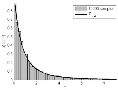
Figure 4: Distribution of the test statistic (6) for the parallelism of two planes. Two point sets withn1 = 4andn2 = 6points have been sampled 10,000 times.
is Fisher-distributed with mand ndegrees of freedom. Here, mdenotes the degrees of freedom for the specific relation, e.g. m = 2for the test of parallelism, andnis the redundancy of the parameter estimation, i.e. the number of equations used to estimate the plane parameters involved in the relation minus the number of unknown plane parameters. The covariance matrix Σddof the contradictionsdis derived by error propagation.
Figure 4 illustrates the distribution of the test statistic (6) check-ing the parallelism of two planes obtained by simulation. We sampled two planes with the rather small number ofn1 = 4and n2= 63D points, estimated the two sets of plane parameters in-dependently, and computed the test statisticdk, see Table 1. The simulation has been performed 10,000 times with uniformly dis-tributed random coordinatesX andY in the interval[0,1]and normal distributed Z-coordinates withσZ = 0.01and mean 0.
As one can see from the histogram, the empirical data fits well to the Fisher-distribution withm= 2andn= 6 + 4−2·3 = 4 degrees of freedom. For larger values ofσZ, the effect of
lin-earization errors become visible.
For the test, we choose the data-independent significance number ofα= 0.05, i.e. the probability of erroneously rejecting the null hypothesis in case it actually holds (type I error). Then the critical valueF1−α;m,n of the corresponding distribution is computed
which limits the regions of acceptance and rejection for the test statistic. The hypothesis will not be rejected ifT < F1−α;m,n
holds for the value of the test statistic (6).
Note that the power of a test, i.e., the probability of not rejecting a null hypothesis while the alternative hypothesis is true, depends also on the sample size.
2.4.2 Pre-Check As one can see from equation (6), the value of the test statistic becomes small if the variance of the distance measure is large. In this case, the null hypothesis tends to be not rejected although the alternative hypothesis is correct (type II error). Therefore, we perform a pre-examination of the data quality by checking the acceptability of the achieved precision for the plane parameters (McGlone et al., 2004). To do so, we pro-vide a reference covariance or criterion matrixCEEfor a plane in canonical formE= [0,0,1,0]T, e.g.
-0.5
vectorN= [0,0,1]T. The confidence region is a hyperboloid of
two sheets, specified by the covariance matrix (7).
plane and a maximum standard deviation of 0.05 m for distance DE = 0of the plane to the origin.
The planes in general orientation are moved to the reference po-sition[0,0,1,0]Tby a 3D motion accompanied by error
propa-gation. For this purpose, the rotation and translation can be ex-tracted from the estimated covariance matrices. The estimate is acceptable if the largest eigenvalue ofΣEEC−1EEis less than or equal to one
λmax ΣEEC−1 EE
≤1, (8)
cf. (McGlone et al., 2004).
2.5 Enforcement of Constraints
For completeness, we provide a brief summary of the utilized ad-justment model. For details please refer to (Meidow, 2014). The solution of the proposed adjustment is equivalent to the adjust-ment with constraints for observations only (Koch, 1999, Mc-Glone et al., 2004). In these models, the existence of a regular covariance matrix for the observations is assumed as its inverse serves as a weight matrix within the adjustment. For the treat-ment of singular covariance matrices, we specialize the general adjustment model introduced in (Meidow et al., 2009).
We compile the unconstrained, spherically normalized parame-ters ofKgiven planes in a parameter vectorx= [AT
1, . . . ,ATK]T
whose singular covariance matrixΣxxfeatures block-diagonal shape. The adjusted or constrained parametersxbare related to the unconstrained parametersxby additive unknown corrections
ǫwhich have to be estimated, thusbx=x+bǫholds.
The functional model subsumes the constraints to be enforced by the adjustment. The intrinsic constraints are the spherical normal-izations (2) of the homogeneous vectors needed to obtain unique results. They are formulated asK restrictionsk(xb) = 0on the parameters. The geometric constraints are theHrestrictions
h(bx) = 0on the plane parameters, e.g. orthogonality or paral-lelism, cf. Table 1.
The stochastic model reflects the uncertainty of the unconstrained parameters, described by an initial block-diagonal covariance matrixΣ(0)xx which results from the parameter estimation (Sub-section 2.2). The covariance matrixΣxxis singular due to over-parametrization. The explicit constraints for the observed planes, i.e., the normalization of the homogeneous entities, and the corre-sponding implicit constraints comprised in the covariance matrix Σxxmust be consistent.
For the derivation of the normal equation system we linearize the constraints. The sought constrained parametersbxare given by the
unconstrained parameters adjusted by estimated correctionsbǫ, or by approximate valuesx0and estimated updates∆x. Thusxb=
x+bǫ=x0+d∆xholds and the linearization of the constraints reads
k(xb) =k(x0) +Kd∆x=Kbǫ+k0 (9)
h(bx) =h(x0) +H∆dx=Hbǫ+h0 (10)
with the JacobiansKandHand the auxiliary variables
k0=k(x0) +K(x−x0) (11)
h0=h(x0) +H(x−x0) . (12)
For the intrinsic constraintsK = Diag(A1,A2, . . . ,AK)and KKT=I holds due to the constraints(AT
kAk−1)/2 = 0for
each entity indexed withk. The JacobianH can be extracted from the equations listed in Table 1.
Minimizing the sum of weighted squared residuals yields the La-grangian
L= 1 2bǫ
TΣ+
xxbǫ+λT(Kbǫ+k0) +µT(Hbǫ+h0) (13) with the Lagrangian vectorsλandµ. Setting the partial deriva-tives of (13) to zero yields the necessary conditions for a mini-mum
∂L ∂bǫT =
Σ+xxbǫ+KTλ+HTµ=0 (14)
and the normal equation system reads
Solving (15) constitutes a solution to the problem at hand but this implies the computation of the pseudo inverse forΣxx, a matrix whose size depends on the number of parameters, i.e., the number of planes. Rewriting (15) leads to the reduced system
Σ+
holds due to the definition of pseudo inverses and the normal equation matrix can be inverted explicitly:
in (10) yields the Lagrangian vectorµ=Σ−1
hh h0−HK
Tk
0 with the regular covariance matrix
Σhh=HΣxxHT (19)
of the small deviations (12) due to variance propagation. Finally we obtain the estimate
bǫ=−Σ for the corrections. Note that the size of the matrix to be inverted depends only on the number of constraints and that the pseudo inverse ofΣxxhas not to be computed explicitly. Furthermore, no special treatment of entities not being affected by any extrinsic constraint is necessary. In this case the corresponding estimates for the corrections (20) will simply be zeros.
The estimates arexb=x+bǫand one has to iterate until con-vergence. Note that the covarianceΣxxmust be adjusted dur-ing the iterations since the linearization points forKchange and ΣxxKT=Omust be fulfilled. This can be achieved by error
Figure 6: RANSAC-based shape detection.
2.6 Deduction of Required Constraints
For the adjustment presented in the previous subsection, a set of consistent, i.e. non-contradicting, and non-redundant constraints is mandatory. Redundant constraints will lead to singular covari-ance matrices (19) for the small deviations. Since we are dealing with imprecise and noisy observations, we have to face the pos-sibility of non-rejected hypotheses which are contradictory, too.
Greedy algorithms are common approaches to select such sets of constraints—either by algebraic methods, e.g. (Loch-Dehbi and Pl¨umer, 2011, Meidow and Hammer, 2016), or by numer-ical methods, e.g. (Pohl et al., 2013). We adopt the approach proposed in (Pohl et al., 2013) to select sets of constraints auto-matically: After adding a constraint, we consider the estimated rank and the estimated condition number of the resulting covari-ance matrix (19). In case of a rank deficiency and/or a small condition number, we neglect the additional constraint.
3. EXPERIMENTS
After introducing the input data, i.e. the utilized point cloud and the derived generic building representation, we illustrate the point sampling, summarize the deduced constraints, and show the re-sults of the adjustment process which enforces the man-made structures.
3.1 Input Data and Point Sampling
We start with the derivation of a generic boundary representa-tion for buildings. Figure 6 shows a detail of an airborne laser scan which represents a rural scene with roofs of farmhouses as dominant man-made objects. The RANSAC-based shape detec-tion (Schnabel et al., 2007) as provided by the 3D point cloud and mesh processing software CLOUDCOMPAREhas been used to extract and group points which are likely to lie on planar facets of the buildings.
Next we derived a generic polyhedral building representation by the procedure proposed in (Xiong et al., 2014). Figure 2 shows the resulting boundary representation which is the input for the proposed reasoning process. Due to the specific reconstruction process, the walls of the buildings are vertical and the bottom area of the building is horizontal. Apart from that, the boundary representation of the roof is unconstrained.
For each facet of the boundary representation we carried out a point sampling by equally spacing points with added noise to the point coordinates (Figure 3). The point spacing ofD= 0.10m and the noise ofσ= 0.03m for point-plane distances simulate the assumed scanning process.
Figure 7: Illustration of all constraints between faces recognized by the hypotheses tests: identity (−·), orthogonality (–), paral-lelism (· · ·), concurrence (◦), verticality (vertical poles). Con-straints with the bottom area of the building are omitted for clar-ity.
constraint number of constraints complete set deduced set
identity 3 0
verticality 27 16
orthogonality 31 7
parallelism 15 2
concurrence 13 13
sum 89 38
Table 2: Recognized and actually required constraints for the ad-justment.
Thresholds influence the degree of generalization for the recon-struction result. However, small facets cannot be avoided in general and a few rather uncertain facets can be created for the boundary representation. The consideration of the uncertainties of the planes with the pre-check proposed in Subsection 2.4.2 al-lows for this.
3.2 Results
Figure 7 illustrates all relations recognized by the hypothesis-generation-and-testing strategy. The utilized constraints for the planes are identity, verticality, orthogonality, parallelism, and
concurrence. The latter considers four planes meeting in a
com-mon 3D point—a situation often encountered in building polyhe-drons. Relations with the bottom area of the building are omitted in Figure 7 for the sake of clarity. Obviously, many relations are redundant, however, it is not clear which can be omitted without loss of information.
Table 2 summarizes the number of recognized and deduced straints itemized according to their type. The set of deduced con-straints is minimal in the sense of consistency and redundancy but the actual number of constraints depends on the order of con-straints as processed by the greedy algorithm. In general, the number of actually required constraints is considerably smaller than the number of recognized constraints.
Figure 8: Constrained boundary representation as the result of the reasoning and adjustment process. 38 functionally independent constraints have been recognized and enforced, cf. Table 2. The reasoning process led to a more adequate representation of the pyramidal broach roof.
4. CONCLUSIONS AND OUTLOOK
The feasibility and usability of the proposed approach has been demonstrated with a first real data set. The only input is a generic boundary representation of a building. Data-dependent thresh-olds are avoided by the exploitation of statistical methods which take the uncertainty of the bounding planes into account.
For the future, several improvements and investigations should be carried out:
• For the simulation of point observations as a result of laser scanning, more sophisticated methods can be envisioned, which take sensor-specific characteristics into account and consider sensor trajectories and scene geometries.
• The formulation of hypotheses for geometric relations should be expanded to express cartographic rules for the generalization of boundary representations as a further ap-plication.
• The estimation of matrix ranks and condition numbers is inexact and becomes unrealizable for large-scale problems. Therefore, algebraic methods should be considered for the deduction of consistent and non-redundant constraints as they provide exact results. Some progress in this regard has been achieved, see (Meidow and Hammer, 2016).
• The set of deduced constraints depends on the order of the constraints within the greedy algorithm. Thus, general rules for the ordering of constraints are advantageous.
• The results depend on the applied point sampling and the adding of noise. This dependency should further be investi-gated.
REFERENCES
Brenner, C., 2005. Constraints for modelling complex objects. Int. Arch. Photogramm. Rem. Sensing 36(3), pp. 49–54.
Bron, C. and Kerbosch, J., 1973. Algorithm 457: finding all cliques of an undirected graph. Communications of the ACM 16(9), pp. 575–577.
Cazals, F. and Karande, C., 2008. A note on the problem of re-porting maximal cliques. Theoretical Computer Science 407(1– 3), pp. 564–568.
F¨orstner, W. and Wrobel, B. P., 2017. Photogrammetric Com-puter Vision – Geometry, Orientation and Reconstruction. Ge-ometry and Computing, Vol. 11, 1stedn, Springer. in press.
F¨orstner, W., Brunn, A. and Heuel, S., 2000. Statistically testing uncertain geometric relations. In: G. Sommer, N. Kr¨uger and C. Perwaß (eds), Mustererkennung 2000, Springer, pp. 17–26.
Heuel, S., 2004. Uncertain Projective Geometry. Statistical Rea-soning in Polyhedral Object Reconstruction. Lecture Notes in Computer Science, Vol. 3008, Springer.
Heuel, S. and Kolbe, T., 2001. Building reconstruction: The dilemma of generic versus specific models. KI – K¨unstliche In-telligenz 3, pp. 75–62.
Koch, K.-R., 1999. Parameter Estimation and Hypothesis Testing in Linear Models. 2ndedn, Springer, Berlin.
Loch-Dehbi, S. and Pl¨umer, L., 2009. Geometric reasoning in 3D building models using multivariate polynomials and charac-teristic sets. Int. Arch. Photogramm. Rem. Sensing Spatial Inf. Sci.
Loch-Dehbi, S. and Pl¨umer, L., 2011. Automatic reasoning for geometric constraints in 3D city models with uncertain observa-tions. ISPRS J. Photogramm. Rem. Sensing 66(2), pp. 177–187.
McGlone, J. C., Mikhail, E. M. and Bethel, J. (eds), 2004. Man-ual of Photogrammetry. 5thedn, American Society of Photogram-metry and Remote Sensing.
Meidow, J., 2014. Geometric reasoning for uncertain observa-tions of man-made structures. In: X. Jiang, J. Hornegger and R. Koch (eds), Pattern Recognition, Lecture Notes in Computer Science, Vol. 8753, Springer, pp. 558–568.
Meidow, J. and Hammer, H., 2016. Algebraic reasoning for the enhancement of data-driven building reconstructions. ISPRS Journal of Photogrammetry and Remote Sensing 114, pp. 179– 190.
Meidow, J., F¨orstner, W. and Beder, C., 2009. Optimal Param-eter Estimation with Homogeneous Entities and Arbitrary Con-straints. In: Pattern Recognition, Lecture Notes in Computer Sci-ences, Vol. 5748, Springer, pp. 292–301.
Pohl, M., Meidow, J. and Bulatov, D., 2013. Extraction and re-finement of building faces in 3D point clouds. In: Image and Signal Processing for Remote Sensing XIX, Society of Photo-Optical Instrumentation Engineers, pp. 88920V–1–10.
Schnabel, R., Wahl, R. and Klein, R., 2007. Efficient RANSAC for point-cloud shape detection. Computer Graphics Forum 26(2), pp. 214–226.
Wu, W., 1986. Basic principles of mechanical theorem proving in elementary geometries. Journal of Automated Reasoning 2, pp. 221–252.
Xiong, B., Jancosek, M., Elberink, S. O. and Vosselman, G., 2015. Flexible building primitives for 3d building modeling. ISPRS Journal of Photogrammetry and Remote Sensing 101, pp. 275–290.

![Figure 5: Plane in canonical form Evector = [0, 0, 1, 0]T with normal N = [0, 0, 1]T. The confidence region is a hyperboloid oftwo sheets, specified by the covariance matrix (7).](https://thumb-ap.123doks.com/thumbv2/123dok/3218837.1394993/4.595.56.289.89.210/figure-plane-canonical-evector-condence-hyperboloid-specied-covariance.webp)